Quantum key distribution with dual detectors

Abstract

To improve the performance of a quantum key distribution (QKD) system, high speed, low dark count single photon detectors (or low noise homodyne detectors) are required. However, in practice, a fast detector is usually noisy. Here, we propose a “dual detectors” method to improve the performance of a practical QKD system with realistic detectors: the legitimate receiver randomly uses either a fast (but noisy) detector or a quiet (but slow) detector to measure the incoming quantum signals. The measurement results from the quiet detector can be used to bound eavesdropper’s information, while the measurement results from the fast detector are used to generate secure key. We apply this idea to various QKD protocols. Simulation results demonstrate significant improvements in both BB84 protocol with ideal single photon source and Gaussian-modulated coherent states (GMCS) protocol; while for decoy-state BB84 protocol with weak coherent source, the improvement is moderate. We also discuss various practical issues in implementing the “dual detectors” scheme.

I Introduction

One important practical application of quantum information is quantum key distribution (QKD), whose unconditional security is based on the fundamental laws of quantum mechanics no_cloning ; BB84 ; E91 ; CV ; nature2003 ; securityproof ; ILD01 ; GLLP . In principle, any eavesdropping attempts by a third party (Eve) will unavoidably introduce quantum bit errors. So, it is possible for the legitimate users (Alice and Bob) to upper bound the amount of information acquired by the eavesdropper given system parameters and the measured quantum bit error rate (QBER). If the QBER is not too high and the transmission efficiency is not too low, Alice and Bob can then distill a final secure key by performing error correction (to correct errors due to imperfections in the QKD system and errors due to eavesdropping) and privacy amplification (to remove Eve’s information on the final key).

A practical QKD system has imperfections, which will contribute to QBER even in the absence of Eve. If Alice and Bob cannot distinguish the intrinsic QBER due to imperfections from the one induced by Eve, in order to guarantee the unconditional security, they have to assume that all errors originate from eavesdropping. Under this assumption, the intrinsic QBER will increase the costs for both error correction and privacy amplification. On the other hand, if Alice and Bob do have a way to distinguish the intrinsic QBER from the one due to eavesdropping, then the cost for the privacy amplification can be reduced Gisin .

One important error source in a practical QKD system is the noise of the receiver’s detector, for example, the dark count probability of a single photon detector (SPD) or the “excess noise” of a homodyne detector. As the distance between Alice and Bob increases (which is equivalent to a higher channel loss), the contribution to QBER from detector’s noise becomes more significant. When the QBER is over some threshold, no secure key can be generated. The maximum secure distance of a QKD system is thus limited by the detector’s noise. On the other hand, the secure key rate is proportional to the operating rate of the QKD system, which is mainly determined by the speed of the detector. In brief, an ideal detector should be fast and noiseless. Unfortunately, in practice, high speed detectors are usually noisy.

In classical metrology, there are many elegant methods to combat various noises associated with the measurement devices. It is natural to ask this question: can we introduce classical “calibration” processes into a QKD system to deal with various noises associated with its intrinsic imperfections? An intuitive idea is as follow: the receiver, Bob, adds a high speed optical switch at the entrance of his device. He uses this switch to randomly block some input signals. The measurement results with no input signal can be used to estimate the intrinsic noise of the detector. Alice and Bob can further estimate among the total QBER (measured when Bob’s switch is open), how much is contributed by this intrinsic detector noise. The QBER caused by the intrinsic detector noise does not contribute to Eve’s information, only the QBER above it does. Since Alice and Bob can bound Eve’s information more tightly, the cost for privacy amplification will be lowered. We remark that the cost for error correction remains the same, because whether the error is caused by eavesdropping or by the intrinsic noise, Alice and Bob will treat them equally during an error correction process.

Note that there is an implicit assumption in the above argument: that Eve cannot control the intrinsic noise of the detector, or at most, she can increase but not decrease it. If Eve can decrease the detector noise when the switch is ON, the above argument is not valid because Bob cannot use the detector noise measured with switch OFF to estimate the detector noise with switch ON. Unfortunately, this assumption is not straightforward to justify. The first rule in quantum cryptography is: to guarantee unconditional secure, one should make assumptions that are most favorable to Eve. In this case, we allow Eve to fully control the noise of Bob’s detectors, and thus the above intuitive idea does not work.

Here we propose a “dual detectors” method to improve the performance of a QKD system based on realistic detectors. The basic idea is quite simple: Bob has two detectors, one is fast but noisy, while the other one is quiet but slow. For each incoming quantum signal, Bob randomly chooses to use either the fast detector (with a high probability) or the slow detector (with a low probability) to do the measurement. During the classical data post-processing stage, Alice and Bob use the QBER measured by the slow (quiet) detector to bound Eve’s information, and they use the raw key bits from the fast detector to produce a secure key. Since Eve cannot predict which detector Bob will choose for each individual bit, her attack is independent on which detector is used. So, Alice and Bob can apply the bound (about Eve’s information) acquired from the low-noise detector to the raw key acquired from the fast (but noisy) detector. By using a tighter bound on Eve’s information, the cost for privacy amplification will be reduced. Intuitively, our proposal will improve the performance of practical QKD setups.

In this paper, we apply the “dual detectors” idea into three different protocols: namely, the BB84 protocol with perfect single photon source BB84 (Section II), the decoy state BB84 protocol with weak coherent source decoy_theory ; Ma05 ; decoy_experiment ; TES2 (Section III), and the Gaussian-modulated coherent states (GMCS) protocol nature2003 (Section IV). Our simulation results confirmed the intuitive prediction of performance, demonstrating significant improvements in both BB84 protocol with an ideal single photon source and GMCS protocol; while for decoy-state BB84 protocol with a weak coherent state source, the improvement is moderate. In Section V, we discuss some practical issues in the implementation of the “dual detectors” idea, including the loss introduced by the optical switch, the distribution of the signals between two detectors, the dispersion of a long fiber and the security of a practical setup. Finally, in Section VI, we end this paper with a brief discussion on the security of a practical QKD system.

II Single photon BB84 QKD with dual detectors

The most well known and mature QKD protocol is BB84 protocol BB84 . There have been a lot of research activities in building a practical single photon source singlephotonsource . In this section, we assume that an ideal single photon source is employed. In this case, the secure key rate is given by GLLP

$$R=\frac{1}{2}rQ_{1}[1-f(e_{1})H_{2}(e_{1})-H_{2}(e_{1})].$$ (1)

Here the factor $1/2$ is due to half of the time, Alice and Bob use different bases (if one uses the efficient BB84 protocol efficient_QKD , this factors is one). $r$ is the pulse repetition rate of the QKD system. $Q_{1}$ is the overall gain (taking into account of channel loss, optical loss inside Bob and the detection efficiency of SPD), which is defined as the ratio of Bob’s detection events to the total signal pulses sent by Alice. $e_{1}$ is the QBER. $f(x)$ is the bidirectional error correction efficiency, and $H_{2}(x)$ is the binary entropy function, given by

$$H_{2}(x)=-x\log_{2}(x)-(1-x)\log_{2}(1-x).$$ (2)

Note that in Eq.(1), the term $f(e_{1})H_{2}(e_{1})$ is the cost for error correction, while the term $H_{2}(e_{1})$ is the cost for privacy amplification. With “dual detectors” method, Alice and Bob use a “quiet” SPD (which yields a lower QBER at a long distance) to give a tighter bound on Eve’s information $H_{2}(e_{1})$. This tighter bound can be used to lower the cost of privacy amplification when Alice/Bob use a “noisier” (but faster) SPD to generate the secure key.

Note the “dual detectors” method cannot be simply explained as using the quiet detector to estimate the dark count of the noisy detector. It should be understood as using the quiet detector to bound Eve’s information more tightly. For each pulse from Alice, right beyond Bob’s optical switch (for randomly choosing detector), Eve’s potential information, $I_{\mathrm{Eve}}^{(0)}$, is independent on which detector Bob will choose to do the measurement. We can imagine Bob’s two detectors as two independent QKD systems. Either of them can upper bound Eve’s information properly. This means the two bounds (on Eve’s information) acquired from the two detectors satisfy: $I_{\mathrm{Eve}}^{(1)}\geq I_{\mathrm{Eve}}^{(0)}$, and $I_{\mathrm{Eve}}^{(2)}\geq I_{\mathrm{Eve}}^{(0)}$. So, Bob can use either of $I_{\mathrm{Eve}}^{(1)}$ (which is quantified by the QBER measured with detector 1) or $I_{\mathrm{Eve}}^{(2)}$ to perform the privacy amplification without compromising the security of the system.

We model the QKD system as follows Ma05 . The gain of the QKD system is

$$Q_{1}=Y_{0}+G_{\mathrm{ch}}G_{\mathrm{Bob}}\eta_{\mathrm{D}}$$ (3)

where $Y_{0}$ is the background rate, $G_{\mathrm{ch}}$ is the channel transmission efficiency, $G_{\mathrm{Bob}}$ is the optical transmittance in Bob’s system, and $\eta_{\mathrm{D}}$ is the efficiency of the SPD. Here we assume that $Y_{0}\ll 1$ and $G_{\mathrm{ch}}G_{\mathrm{Bob}}\eta_{\mathrm{D}}\ll 1$. The quantum channel between Alice and Bob is telecom fiber with attenuation $\alpha=0.21\mathrm{dB/km}$. The channel efficiency can be estimated by $G_{\mathrm{ch}}=10^{-\alpha L/10}$, where $L$ is the fiber length in km.

The QBER is determined by

$$e_{1}=\frac{e_{0}Y_{0}+e_{\mathrm{det}}G_{\mathrm{ch}}G_{\mathrm{Bob}}\eta_{\mathrm{D}}}{Q_{1}}$$ (4)

Here $e_{0}=0.5$ is the error rate of background counts, which is dominated by dark counts Dark_count , and $e_{\mathrm{det}}$ is the probability that a single photon hits the wrong detector when Alice and Bob choose the same basis. $e_{\mathrm{det}}$ characterizes the alignment and the stability of the optical system and the cross-talk between adjacent signals, etc.

We assume that Bob randomly chooses to use one of the following two SPDs: the first one is fast but noisy (with operating rate $r_{1}$, efficiency $\eta_{\mathrm{D}}^{(1)}$ and dark count probability $Y_{0}^{(1)}$), while the second one is slow but quiet (with operating rate $r_{2}$, efficiency $\eta_{\mathrm{D}}^{(2)}$ and dark count probability $Y_{0}^{(2)}$ ). To improve the overall efficiency (only the fast SPD contributes to the final secure key), the probability of choosing the slow SPD should be small (in asymptotic case, it can approach zero). The secure key rate of the “dual detectors” scheme is given by

$$R=\frac{1}{2}r_{1}Q_{1}^{(1)}[1-f(e_{1}^{(1)})H_{2}(e_{1}^{(1)})-H_{2}(e_{1}^{(2)})].$$ (5)

Here, $e_{1}^{(1)}$ and $e_{1}^{(2)}$ are the QBERs measured by SPD1 and SPD2, respectively.

Numerical simulations have been performed based on different combinations of SPDs.

II.1 Case One: up-conversion SPD and transition-edge sensor SPD

Two different types of SPD are employed in this case. SPD1 is a high speed SPD based on up-conversion process. Recently, these MHz devices have been employed in GHz rate QKD systems upconversion1 ; upconversion2 . SPD2 is a “low noise” SPD based on transition-edge sensors (TESs) TES1 ; TES2 . Simulation parameters are summarized as follows: $\alpha=0.21\mathrm{dB/km}$, $f(x)=1.22$; $G_{\mathrm{Bob}}=0.16$ and $e_{\mathrm{det}}=0.018$ TES1 ; $r_{1}=1\mathrm{GHz}$, $\eta_{\mathrm{D}}^{(1)}=0.059$ and $Y_{0}^{(1)}=1.3\times 10^{-5}$ upconversion2 ; $r_{2}=2.5\mathrm{MHz}$, $\eta_{\mathrm{D}}^{(2)}=0.5$ and $Y_{0}^{(2)}=3\times 10^{-7}$TES2 .

Fig.1 shows the simulation results. The key rate of “dual-detector” system is higher than either of the two single SPD systems up to $\sim 124\mathrm{km}$. Note that, at a long distance, the system with SPD2 alone yields a higher key rate than a dual-detector system. Thus Bob can simply use SPD2 alone.

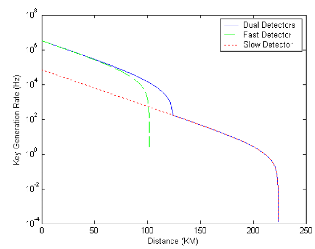
Figure 1: Simulation results for BB84 protocol with single photon source. Simulation parameters: $\alpha=0.21\mathrm{dB/km}$, $f(x)=1.22$; $G_{\mathrm{Bob}}=0.16$ and $e_{\mathrm{det}}=0.018$ TES1 ; $r_{1}=1\mathrm{GHz}$, $\eta_{\mathrm{D}}^{(1)}=0.059$ and $Y_{0}^{(1)}=1.3\times 10^{-5}$ upconversion2 ; $r_{2}=2.5\mathrm{MHz}$, $\eta_{\mathrm{D}}^{(2)}=0.5$ and $Y_{0}^{(2)}=3\times 10^{-7}$TES2 . The key rate of “dual detectors” system is higher than either of the two single SPD systems up to $\sim 124\mathrm{km}$. Note that at a longer distance, when the system with SPD2 alone yields a higher key rate, Bob can simply use SPD2 itself.

II.2 Case Two: low jitter up-conversion SPD and transition-edge sensor SPD

In this case, we assume that SPD1 is a low jitter up-conversion SPDSPD_10G1 , which has been applied in a $10\mathrm{GHz}$ QKD system SPD_10G2 . Note that, in this case, due to the high pulse repetition rate and non-zero time jitter, the cross-talk between adjacent pulses is high. This contributes to a high QBER independent of fiber length, which is equivalent to a high $e_{\mathrm{det}}$ for SPD1. The parameters for SPD1 are: $r_{1}=10\mathrm{GHz}$, $\eta_{D}^{(1)}=0.0027$, $Y_{0}^{(1)}=3.2\times 10^{-9}$ and $e_{\mathrm{det}}^{(1)}=0.097$ SPD_10G2 . Other parameters are the same as in Case One.

Fig.2 shows the simulation results. The key rate of the “dual detectors” system is significantly higher than either of the two single SPD systems up to $\sim 200\mathrm{km}$. Here we particularly remark that no secure key can be produced by SPD1 alone at any distance.

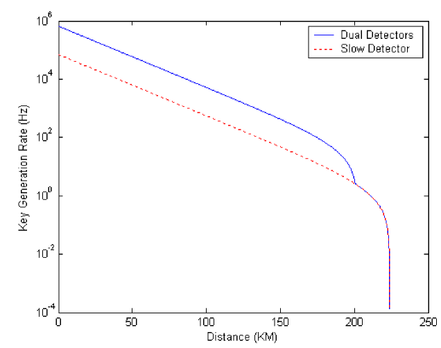
Figure 2: Simulation results for BB84 protocol with single photon source. Simulation parameters: $r_{1}=10\mathrm{GHz}$, $\eta_{\mathrm{D}}^{(1)}=0.0027$, $Y_{0}^{(1)}=3.2\times 10^{-9}$ and $e_{\mathrm{det}}^{(1)}=0.097$ SPD_10G2 . Other parameters are same as in Fig.1. The key rate of “dual detectors” system is significantly higher than either of the two single SPD systems up to $\sim 200\mathrm{km}$. Note that no secure key can be produced by SPD1 alone at any distance.

II.3 Case Three: two low jitter up-conversion SPDs

In Case One and Case Two, the working principles of the two SPDs are substantially different. To prevent Eve from exploring the difference between the two detectors, special counter measures, such as narrowband filters, may be required. We will discuss this topic in details in Section V.

In Case Three, two identical low jitter SPDs are employed to remove the asymmetry between the two detectors. The probability for choosing SPD1 is close to one. So, it still suffers from the high QBER due to the cross-talk between adjacent pulses. Since the probability for choosing SPD2 is quite small (say $<0.01$), the cross-talk between adjacent pulses can be neglected, and the QBER from SPD2 will be much lower. Simulation parameters are summarized as follows: $r_{1}=10\mathrm{GHz}$, $\eta_{\mathrm{D}}^{(1)}=0.0027$, $Y_{0}^{(1)}=3.2\times 10^{-9}$ and $e_{\mathrm{det}}^{(1)}=0.097$ SPD_10G2 . $r_{2}=100\mathrm{MHz}$, $\eta_{\mathrm{D}}^{(2)}=0.0027$, $Y_{0}^{(2)}=3.2\times 10^{-9}$ and $e_{\mathrm{det}}^{(2)}=0.018$. Other parameters are the same as before.

Fig.3 shows the simulation results. The key rate of the “dual detectors” system is significantly higher than either of the two single SPD systems up to $\sim 190\mathrm{km}$. Again, no secure key can be produced by SPD1 alone at any distance.

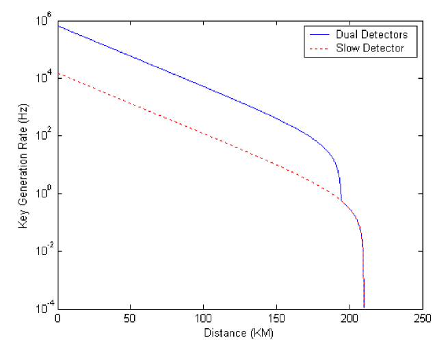
Figure 3: Simulation results for BB84 protocol with single photon source. Simulation parameters: $r_{1}=10\mathrm{GHz}$, $\eta_{\mathrm{D}}^{(1)}=0.0027$, $Y_{0}^{(1)}=3.2\times 10^{-9}$ and $e_{\mathrm{det}}^{(1)}=0.097$ SPD_10G2 ; $r_{2}=100\mathrm{MHz}$, $\eta_{\mathrm{D}}^{(2)}=0.0027$, $Y_{0}^{(2)}=3.2\times 10^{-9}$ and $e_{\mathrm{det}}^{(2)}=0.018$; Other parameters are same as in Fig.1. The key rate of “dual detectors” system is significantly higher than either of the two single SPD systems up to $\sim 190\mathrm{km}$. Note that no secure key can be produced by SPD1 alone at any distance.

In summary, our simulation results demonstrate that the “dual detectors” method can improve the performance of single photon BB84 QKD system dramatically. We remark that the same idea can also be applied to QKD with imperfect single photon sources.

III Decoy state BB84 QKD with dual detectors

Currently, most of QKD experiments are performed with a weak coherent source. The photon number of each pulse follows a Poisson distribution with a parameter $\mu$ as its expected photon number, which is set by Alice. In this case, the secure key rate is given by GLLP

$$R=\frac{1}{2}r[Q_{1}-f(E_{\mu})Q_{\mu}H_{2}(E_{\mu})-Q_{1}H_{2}(e_{1})].$$ (6)

Here $Q_{\mu}$, $E_{\mu}$ are the gain and the overall QBER of signal states, while $Q_{1}$, $e_{1}$ are the gain and the QBER of single-photon components. Note that only $Q_{\mu}$, $E_{\mu}$ can be determined from experimental data directly, while the bounds on $Q_{1}$ and $e_{1}$ have to be estimated from the specific QKD protocol and model of QKD system.

Here, we assume that Alice and Bob perform ideal decoy state BB84 protocol decoy_theory ; Ma05 . In the asymptotic case, the estimated value of the above four parameters are given by Ma05

$$Q_{\mu}=Y_{0}+1-e^{-\eta\mu}$$ (7)

$$E_{\mu}=[e_{0}Y_{0}+e_{\mathrm{det}}(1-e^{-\eta\mu})]/Q_{\mu}$$ (8)

$$Q_{1}=(Y_{0}+\eta)\mu e^{-\mu}$$ (9)

$$e_{1}=(e_{0}Y_{0}+e_{\mathrm{det}}\eta)\mu e^{-\mu}/Q_{1}$$ (10)

Here $\eta=G_{\mathrm{ch}}G_{\mathrm{Bob}}\eta_{\mathrm{D}}$ is the overall efficiency of the QKD system.

The optimal $\mu$ for the signal state can be estimated from Ma05

$$(1-\mu)e^{-\mu}=\frac{f(E_{\mu})H_{2}(e_{\mathrm{det}})}{1-H_{2}(e_{\mathrm{det}})}$$ (11)

With the “dual detectors” method, we expect that Alice and Bob can obtain a tighter bound on $e_{1}$, thus lowering the cost of privacy amplification. Simulation parameters are summarized as follows: $\alpha=0.21\mathrm{dB/km}$, $f(x)=1.22$, $\mu=0.73$ ; $G_{\mathrm{Bob}}=0.16$ and $e_{\mathrm{det}}=0.018$ TES1 ; $r_{1}=1\mathrm{GHz}$, $\eta_{\mathrm{D}}^{(1)}=0.059$ and $Y_{0}^{(1)}=1.3\times 10^{-5}$ upconversion2 ; $r_{2}=2.5\mathrm{MHz}$, $\eta_{\mathrm{D}}^{(2)}=0.5$ and $Y_{0}^{(2)}=3\times 10^{-7}$ TES2 . The optimal $\mu$ in the case of “dual detectors” is chosen based on the parameters of the fast detector. The simulation results are shown in Fig.4. We see moderate improvement up to $\sim 82\mathrm{km}$.

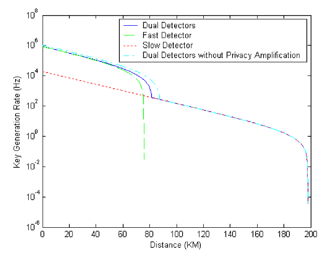
Figure 4: Simulation results for Decoy state BB84 protocol with weak coherent source: Simulation parameters: $\alpha=0.21\mathrm{dB/km}$, $f(x)=1.22$, $\mu=0.73$; $G_{\mathrm{Bob}}=0.16$ and $e_{\mathrm{det}}=0.018$ TES1 ; $r_{1}=1\mathrm{GHz}$, $\eta_{\mathrm{D}}^{(1)}=0.059$ and $Y_{0}^{(1)}=1.3\times 10^{-5}$ upconversion2 ; $r_{2}=2.5\mathrm{MHz}$, $\eta_{\mathrm{D}}^{(2)}=0.5$ and $Y_{0}^{(2)}=3\times 10^{-7}$TES2 .The key rate of “dual detectors” system is higher than either of the two single SPD systems up to $\sim 82\mathrm{km}$. Note that even without doing any privacy amplification, the improvement in this case is moderate.

The limited improvement in this protocol can be understood from Eq.(6). The second term ($f(E_{\mu})Q_{\mu}H_{2}(E_{\mu})$) at the right hand side of Eq.(6) is the cost for error correction, while the third term ($Q_{1}H_{2}(e_{1})$) is the cost for privacy amplification. Since $f(E_{\mu})Q_{\mu}H_{2}(E_{\mu})$ is significantly larger than $Q_{1}H_{2}(e_{1})$, the cost of the error correction term is the dominating factor. The “dual detectors” system only allows us to reduce the privacy amplification term, but not the error correction term. Therefore, any improvement due to the “dual detectors” system for decoy state BB84 protocol over telecom fibers will be moderate. This point is clearly illustrated by our numerical simulations in Fig.4: even if Alice and Bob did not perform any privacy amplification, the improvements in secure key rate and secure distance would still be moderate.

IV Gaussian-modulated coherent states QKD with dual detectors

Recently, GMCS QKD has drawn a lot of attention for its potential high secure key rate, especially at relatively short distance nature2003 ; dr ; rr ; GMCS ; PP . In this protocol nature2003 , Alice draws two random numbers $X_{A}$ and $P_{A}$ from a Gaussian distribution with mean zero and variance $V_{A}$ (in shot-noise units), and sends a coherent state $|X_{A}+iP_{A}\rangle$ to Bob. Bob randomly chooses to measure either the phase quadrature or the amplitude quadrature with a phase modulator and a homodyne detector. During the classical communication stage, Bob informs Alice which quadrature he measures for each pulse and Alice will drop the other one. Eventually, they can work out a set of correlated Gaussian variables, which will be converted to a secure key. It has been shown in nature2003 that with “reverse reconciliation” (RR) protocol rr , this scheme can tolerate high channel loss on the condition that the excess noise (the noise above vacuum noise) is not too high, while with “direct reconciliation” (DR) protocol dr , this scheme can yield a high key rate at relatively short distances.

IV.1 Direct Reconciliation Protocol

We assume symmetry on the noise characteristics between the amplitude quadrature measurement and phase quadrature measurement. For additive Gaussian noise channels, the mutual information between Alice and Bob, $I_{AB}$, and between Alice and Eve, $I_{AE}$, are given by dr

$$I_{AB}=(1/2)\log_{2}[(V+\chi)/(1+\chi)]$$ (12)

$$I_{AE}=(1/2)\log_{2}[(V+1/\chi)/(1+1/\chi)]$$ (13)

where $V=V_{A}+1$ is the variance of Alice’s field quadratures in shot-noise units, $\chi=\chi_{\mathrm{vac}}+\varepsilon$ is the equivalent input noise, where $\chi_{\mathrm{vac}}=(1-G)/G$ is the “vacuum noise” associated with the overall transmission efficiency $G$, while $\varepsilon$ is the “excess noise”. $G=G_{\mathrm{ch}}G_{\mathrm{det}}$, where $G_{\mathrm{ch}}$ is the channel efficiency and $G_{\mathrm{det}}$ is the detection efficiency.

Note that since $\varepsilon$ is the “excess noise” with respect to the input, it can be described by $\varepsilon=\varepsilon_{\mathrm{pre}}+\varepsilon_{\mathrm{det}}/G$, where $\varepsilon_{\mathrm{pre}}$ and $\varepsilon_{\mathrm{det}}$ are the “excess noises” associated with imperfections in state preparation and homodyne detection, respectively. Obviously, at long distances (i.e., $G$ is small), the main contribution to $\varepsilon$ is from the detector noise.

The security key rate of a DR protocol is given by dr

$$R_{1}=r(\beta I_{AB}-I_{AE})$$ (14)

where $r$ is the repetition rate of the QKD system and $\beta\in(0,1)$ is the efficiency of DR protocol.

In GMCS QKD system, the “excess noise” plays a similar role as the dark count probability of SPD in BB84 protocol. The “dual detectors” scheme can be employed to improve the performance of a GMCS QKD system based on realistic homodyne detectors, as in the case of BB84 protocol. Specifically, at the classical communication stage, Alice and Bob use the measurement results from the quiet detector and Eq.(13) to estimate $I_{AE}$ and the measurement results from the fast detector and Eq.(12) to calculate $I_{AB}$. Using Eqs.(12-14), the secure key rate of the “dual detectors” scheme can be derived as

$$R_{2}=r_{1}\{(\beta/2)\log_{2}[(V+\chi_{\mathrm{vac}}+\varepsilon_{1})/(1+\chi_{\mathrm{vac}}+\varepsilon_{1})]$$

$$-(1/2)\log_{2}[(V+1/(\chi_{\mathrm{vac}}+\varepsilon_{2}))/(1+1/(\chi_{\mathrm{vac}}+\varepsilon_{2}))]\}$$ (15)

Simulation parameters are summarized as follows: $\alpha=0.21\mathrm{dB/km}$, $V=40$, $\beta=1$, $G_{\mathrm{det}}=0.80$; $\varepsilon_{\mathrm{pre}}=0.05$GMCS ; $r_{1}=82\mathrm{MHz}$, $\varepsilon_{\mathrm{det1}}=0.43$ fasthom ; $r_{2}=1\mathrm{MHz}$, $\varepsilon_{\mathrm{det2}}=0.01$GMCS .

Fig.5 shows the simulation results. With the “dual detectors” method, we see a significant improvement of the key rate (more than one order) at relatively short distance (up to $5$km).

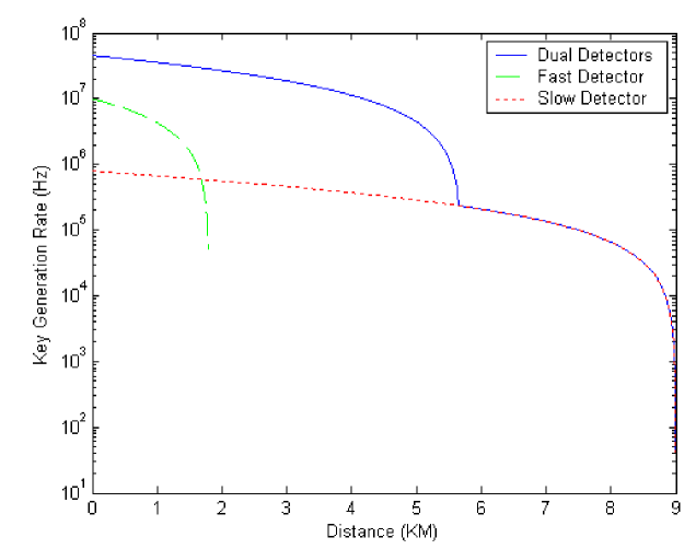
Figure 5: Simulation results for GMCS QKD with DR protocol. Simulation parameters: $\alpha=0.21\mathrm{dB/km}$, $V=40$, $\beta=1$; $G_{\mathrm{det}}=0.8$, $\varepsilon_{\mathrm{pre}}=0.05$GMCS ; $r_{1}=82\mathrm{MHz}$, $\varepsilon_{\mathrm{det1}}=0.43$ fasthom ; $r_{2}=1\mathrm{MHz}$, $\varepsilon_{\mathrm{det2}}=0.01$GMCS . With the “dual-detectors” method, we see a significant improvement of the key rate (more than one order of magnitude) at relatively short distance(up to $5$km).

IV.2 Reverse Reconciliation Protocol

In RR protocols, Bob sends classical information to Alice, who in turn modifies her initial data to match with Bob’s measurement results. The security key rate of a RR protocol is given by nature2003 ; GMCS

$$R_{1}=r(\beta I_{BA}-I_{BE})$$ (16)

where the mutual information between Bob and Alice, $I_{BA}$, and between Bob and Eve, $I_{BE}$, are given by nature2003

$$I_{BA}=(1/2)\log_{2}[(V+\chi)/(1+\chi)]$$ (17)

$$I_{BE}=(1/2)\log_{2}[G^{2}(V+\chi)(V^{-1}+\chi)]$$ (18)

We remark that to derive the above equations, Eve is allowed to control both the efficiency and excess noise in Bob’s system. In contrast, in nature2003 ; GMCS , the authors took a “realistic” approach by assuming that the noises associated with Bob’s system do not contribute to Eve’s information.

We remark that there is a substantial difference between GMCS QKD with DR protocol and GMCS QKD with RR protocol. In DR protocol, Alice/Bob try to bound the mutual information between Alice and Eve $I_{AE}^{(0)}$, which is independent on the performance of Bob’s measurement device. Due to the noise and loss presented in Bob’s system, they will overestimate $I_{AE}^{(0)}$ as $I_{AE}^{(1)}$ (with detector1) or $I_{AE}^{(2)}$ (with detector2). Obviously, they can use $\mathrm{min}\{I_{AE}^{(1)},I_{AE}^{(2)}\}$ as an estimation of $I_{AE}^{(0)}$ in Eq.(14). In “reverse reconciliation” method, the above argument cannot be applied. In this case, Alice/Bob try to bound the mutual information between Bob and Eve $I_{BE}$, which depends on both the efficiency and the noise of the homodyne detector (see Eq.(18), where the overall transmission efficiency $G$ contains contribution from the efficiency of the homodyne detector ). If the efficiencies of the two detectors are different, Eve’s information on Bob’s measurement results acquired with detector1 may be different from her information on Bob’s measurement results acquired with detector2. In order to use the slow detector to give a better bound on $I_{BE}$ for the data acquired with the fast detector, we have to assume that both detectors have the same efficiency. Note that this is a reasonable assumption in practice, since the efficiency of the homodyne detector is mainly determined by two factors—the optical coupling efficiency and the quantum efficiency of the photo diode. Both factors are insensitive to the operation rate.

We remark that transmission loss plays different roles in different QKD protocols. In GMCS QKD, the transmission loss will introduce “vacuum noise” to Bob’s measurement results, and Bob cannot distinguish this “vacuum noise” from the “excess noise” contributed by the homodyne detector or other imperfections in the QKD system. To bound Eve’s information on Bob’s measurement results, Alice and Bob have to estimate both the efficiency of the QKD system and the “excess noise”. On the other hand, in BB84 QKD, since Alice/Bob post-select the cases when Bob has detections (they drop all the other cases), the transmission loss only lower the efficiency but not contribute to the QBER. To bound Eve’s information, Alice/Bob only need to estimate the QBER. This may explain why in BB84 QKD, to apply the “dual detectors” idea, it is no necessary to make assumptions on the efficiencies of the two detectors.

The secure key rate of the “dual detectors” scheme can be derived as

$$R_{2}=r_{1}\{(\beta/2)\log_{2}[(V+\chi_{\mathrm{vac}}+\varepsilon_{1})/(1+\chi_{\mathrm{vac}}+\varepsilon_{1})]$$

$$-(1/2)\log_{2}[G^{2}(V+\chi_{\mathrm{vac}}+\varepsilon_{2})(V^{-1}+\chi_{\mathrm{vac}}+\varepsilon_{2})]\}$$ (19)

Simulation parameters are the same as in DR protocol. Fig.6 shows the simulation results. With the “dual detectors” method, we see a significant improvement of the key rate (more than one order of magnitude) at relatively short distance (up to $17$km). Note that, in this case, no positive key rate can be achieved with detector1 alone at any distance.

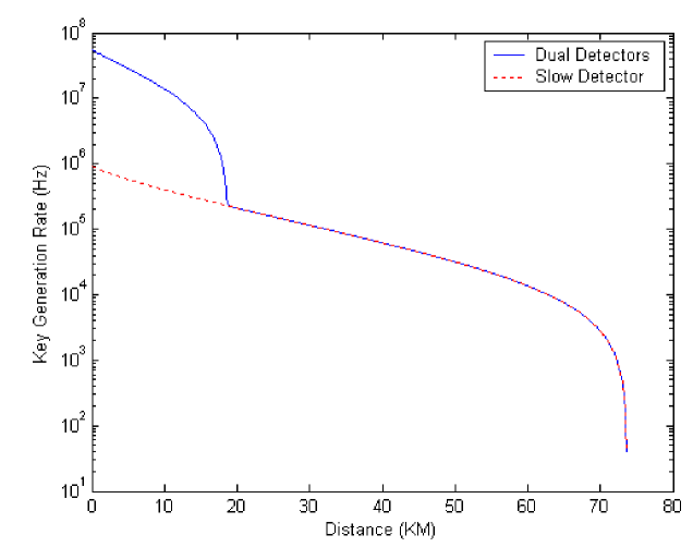
Figure 6: Simulation results for GMCS QKD with RR protocol. Simulation parameters: $\alpha=0.21\mathrm{dB/km}$, $V=40$, $\beta=1$; $G_{\mathrm{det}}=0.8$, $\varepsilon_{\mathrm{pre}}=0.05$GMCS ; $r_{1}=82\mathrm{MHz}$, $\varepsilon_{\mathrm{det1}}=0.43$ fasthom ; $r_{2}=1\mathrm{MHz}$, $\varepsilon_{\mathrm{det2}}=0.01$GMCS . With the “dual-detectors” method, we see a significant improvement of the key rate (more than one order of magnitude) at relatively short distance(up to $17$km). Note that in this case, no positive key rate can be achieved with detector1 alone at any distance.

In practice, for a finite key length, the reconciliation algorithm is not perfect. Fig.7 shows the simulation results with a realistic RR protocol ($V=20$, $\beta=0.8$, other parameters are the same as in Fig.6). With the “dual detectors” method, we see a significant improvement of the key rate (more than one order of magnitude) at relatively short distance (up to $5$km). Again, no positive key rate can be achieved with detector1 alone at any distance.

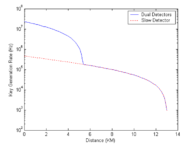
Figure 7: Simulation results for GMCS QKD with realistic RR protocol. Simulation parameters: $\alpha=0.21\mathrm{dB/km}$, $V=20$, $\beta=0.8$; $G_{\mathrm{det}}=0.8$, $\varepsilon_{\mathrm{pre}}=0.05$GMCS ; $r_{1}=82\mathrm{MHz}$, $\varepsilon_{\mathrm{det1}}=0.43$ fasthom ; $r_{2}=1\mathrm{MHz}$, $\varepsilon_{\mathrm{det2}}=0.01$GMCS . With the “dual-detectors” method, we see a significant improvement of the key rate (more than one order of magnitude) at relatively short distance(up to $5$km). Note that in this case, no positive key rate can be achieved with detector1 alone at any distance.

We remark that the above security analysis about GMCS QKD, which are cited from nature2003 , may be applicable to individual attacks only. The security of GMCS protocol under the most general attack is still under investigation GMCS_security .

V Practical issues

In this section, we will discuss several practical issues in implementing the “dual detector” idea, including the loss introduced by the optical switch, the probability of using each type of detectors, the chromatic dispersion of long fiber and the security of a practical setup.

In previous sections, we assume that Bob has an ideal, lossless optical switch to distribute the incoming pulses between the two detectors. A commercial high speed optical switch designed for telecom industry has a insertion loss around 3dB. To make a fair comparison, we introduce an additional 3dB loss in Bob’s system for “dual detector” scheme. The simulation results demonstrate that in the case of single photon QKD, the advantage of “dual detector” is still obvious, as shown in Fig.8 and Fig.9, while in the case of decoy state QKD and GMCS QKD, the additional 3dB loss is disastrous: with the parameters used in Sections 3 and 4, the “dual detector” scheme shows no advantage over conventional “single detector” scheme. This result is not surprising: for decoy-state QKD, even with a perfect lossless switch, the improvement is quite limited (see Fig.4); for GMCS QKD, we already know that the key rate drops sharply as the channel loss increase nature2003 .

We remark that the 3dB loss of a commercial high speed optical switch is mostly due to the fiber-waveguide coupling loss, which is by no means a hard limit imposed by the technology. In fact, if only one wavelength channel is used for QKD, one could optimize waveguide design to minimize coupling loss. In this case, one can reasonably expect the insertion loss to be much lower than 1dB, at a higher price.

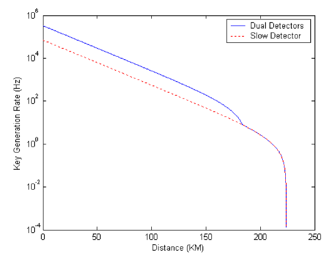
Figure 8: Simulation results with a lossy (3dB) optical switch. Simulation parameters: $r_{1}=10\mathrm{GHz}$, $\eta_{\mathrm{D}}^{(1)}=0.0027$, $Y_{0}^{(1)}=3.2\times 10^{-9}$ and $e_{\mathrm{det}}^{(1)}=0.097$ SPD_10G2 . Other parameters are same as in Fig.1. The key rate of “dual detectors” system is significantly higher than either of the two single SPD systems up to $\sim 180\mathrm{km}$. Note that no secure key can be produced by SPD1 alone at any distance.

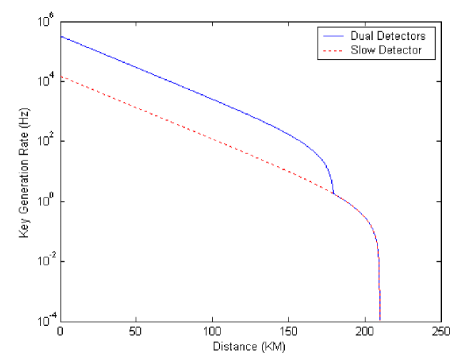
Figure 9: Simulation results with a lossy (3dB) optical switch. Simulation parameters: $r_{1}=10\mathrm{GHz}$, $\eta_{\mathrm{D}}^{(1)}=0.0027$, $Y_{0}^{(1)}=3.2\times 10^{-9}$ and $e_{\mathrm{det}}^{(1)}=0.097$ SPD_10G2 ; $r_{2}=100\mathrm{MHz}$, $\eta_{\mathrm{D}}^{(2)}=0.0027$, $Y_{0}^{(2)}=3.2\times 10^{-9}$ and $e_{\mathrm{det}}^{(2)}=0.018$; Other parameters are same as in Fig.1. The key rate of “dual detectors” system is significantly higher than either of the two single SPD systems up to $\sim 175\mathrm{km}$. Note that no secure key can be produced by SPD1 alone at any distance.

Another important issue is how to determine the probability of using each of the two detectors. Since only the output from the fast detector contributes to the final key, in asymptotic limit, the probability of using the slow detector should be as small as possible. In practice, two other factors have to be taken into account. First, in order to estimate the system parameters accurately, Alice/Bob have to acquire enough data for either type of detectors in a reasonable time period. This determines the lower bound on the probability for choosing the slow detector. Second, the slow detector may have a large time jitter. If more than one pulses are sent to it within its response window, Bob cannot tell which incoming pulse the detection event corresponds to and the QBER will increase. This determines the upper bound on the probability of choosing the slow detector. In the following, we will estimate the probability $p$ of choosing the slow detector (detector2) based on the parameters of a practical setup.

We assume the period of the signal pulse is $T_{\mathrm{sig}}$, and the time resolution (time jitter) of detector2 is $T_{\mathrm{det}}$. In each single response window of detector2, there are $k$ ($=T_{\mathrm{det}}/T_{\mathrm{sig}}$) pulses sent out by Alice. Bob randomly chooses to use either detector1 (with a probability of $1-p$) or detector2 (with a probability of $p$) to measure the input pulse. In each $T_{\mathrm{det}}$ time window, the probabilities that Bob does not choose detector2, chooses it one time, or chooses it more than one time are $P_{0}$ ($=(1-p)^{k}$), $P_{1}$ ($=kp(1-p)^{k-1}$) and $P_{M}$ ($=1-P_{0}-P_{1}$), respectively. Assuming that $p\ll{k}\ll{1}$, we have $P_{1}=kp-k(k-1)p^{2}$ and $P_{M}=k(k-1)p^{2}/2$. Note that the probability that Bob chooses detector2 only one time (in the $T_{\mathrm{det}}$ time window)and he does detect a signal is $P_{\mathrm{sig}}=\mu\eta P_{1}$, where $\mu$ is the average photon number per pulse, and $\eta$ is the overall transmission efficiency (including the channel efficiency, the optical transmittance in Bob’s system, and the efficiency of detector2). This is an effective detection. On the other hand, if Bob chooses detector2 more than one time and he does detect a signal, then he has to randomly assign this detection event to one of the input pulses he chooses. If we assume that the major contribution to $P_{M}$ comes from $P_{2}$, then the probability for Bob to get a “messed detection” is $P_{\mathrm{err}}=2\mu\eta P_{M}$, where the factor $2$ takes into account that two pulses have been sent to detector2. The error rate of these “messed detection” is $1/4$, because half of the time, Bob will assign the detection event to the right pulse (no error), the other half of time, Bob will assign the detection event to the wrong pulse ($1/2$ error). The overall QBER due to the “multi-pulses” problem can be estimated as

$$QBER\approx\frac{P_{\mathrm{err}}}{4(P_{\mathrm{err}}+P_{\mathrm{sig}})}\approx\frac{1}{4}(k-1)p$$ (20)

Using parameters in Fig.1, $T_{\mathrm{det}}=100ns$ TES2 , $T_{\mathrm{sig}}=1ns$ ($1\mathrm{GHz}$ pulse repetition rate), we have $k=100$. To make the additional $QBER<1\%$, we get $p<4\times 10^{-4}$. On the other hand, if we assume the channel loss is 21dB (100km fiber), $G_{\mathrm{Bob}}=0.16$, $\eta_{\mathrm{D}}^{(2)}=0.5$, the additional loss due to optical switch is 3dB, then, with $p=4\times 10^{-4}$ and $1\mathrm{GHz}$ pulse repetition rate, Bob will have $\sim 10^{6}$ counts in about 2 hours, which is large enough to estimate various parameters of the QKD system stat_flu . In Fig.3, since both detectors have small time jitter, the $p$ value can be relatively large.

We remark that the minimum $p$ achievable in practice is limited by the extinction ratio of the optical switch. On the other hand, it may be possible to overcome this “multi pulses” problem by improving the protocol. For example, Bob can prepare his random pattern for the optical switch in the following way: if the $n_{th}$ pulse is assigned to the slow detector, then the next $r$ pulses ($r$ is determined by the time resolution of the slow detector) will not be assigned to it. This is equivalent to introducing a “virtual dead time” to the slow detector. It is interesting to investigate the security of this scheme. However, we do not have a definite answer so far.

We remark that the slow response of detector2 also prevents Bob from using a passive beam splitter to replace the optical switch. In that case, Bob cannot tell which input pulse corresponds to the detection event from detetor2.

The third practical issue is the chromatic dispersion introduced by the telecom fiber. The chromatic dispersion of conventional telecom fiber at $1550\mathrm{nm}$ is around $18\mathrm{ps/nm}\cdot{\mathrm{km}}$. In many QKD system, the spectral width of the laser pulse is in the order of $0.1\mathrm{nm}$, so the temporal pulse width will be extended by $180\mathrm{ps}$ after it goes through $100\mathrm{km}$ fiber. This will cause severe cross talks between adjacent pulses when the system is operated at $10\mathrm{GHz}$. We remark that dispersion compensation (DC) is an important issue even in classical communication, and various successful DC techniques have been developed. For example, in dispersion , after going through a 50km fiber, a 460fs pulse was only slightly broadened to 470fs. Similar techniques can also be applied to a QKD system. We remark that the loss introduced by DC components will not compromise the performance of the QKD system, since it can be deployed inside Alice’s system.

An important assumption of our “dual detector” idea is that a signal from Eve cannot fool the two detectors by behaving differently. Such an assumption must not be taken for granted. Instead, it should be examined carefully in any practical system. However, we note that there are various defense strategies that Alice and Bob can employ to make our assumption more realistic. For instance, to prevent Eve from attacking the two detectors differently by sending laser pulses at different wavelengths, Bob has to make sure that the spectral responses of the two detectors are identical to Eve. Normally, a photon detector has a spectral response range from tens of nm to larger than 100nm, while the spectral width of the laser pulse from Alice is less than 1nm. By placing a narrowband optical filter (with a bandwidth of $\sim 1\mathrm{nm}$) at the entrance of Bob’s system, we can safely assume that the spectral responses of both detectors are flat in this spectral window filter . On the other hand, Eve may explore the different temporal responses of the two detectors by shifting the arriving time of the laser pulse time-shift . For example, in the case of up-conversion SPD, to achieve a low dark count, Bob uses narrow time windows, which are centered around the incoming pulses, to post-select effective detection events. All detection events outside these time windows will be dropped. If the widths of time windows are different for the two detectors, Eve may time-shift a pulse in such a way that one detector will treat it as an effective event, while the other one will drop it. We remark that to prevent Eve from launching such a time-shift attack, Bob should monitor the time distribution of all his detection events.

VI Discussion

The performance of a QKD system in telecom wavelength is mainly determined by the performance of its detection system. To achieve high speed, long distance QKD, fast and quiet detectors are on demand. Unfortunately, in practice, a fast detector is usually more noisy than a slow one. Here, we propose a “dual detectors” scheme to improve the performance of a practical QKD system with realistic detectors. Our simulation results demonstrate significant improvements of the secure key rate in some QKD protocols.

Any security proof of a practical QKD system is built on its underlying assumptions: what kinds of imperfections exist, what Eve can control/know about Alice’s and Bob’s systems. Obviously, if we allow Eve to control/know everything (like which SPD clicks in BB84 QKD), secure QKD is hopeless. On the other hand, people normally assume that the loss inside Bob’s system and the dark count of Bob’s SPD are under Eve’s control. In this case, secure QKD is still possible. Unfortunately, in practice, there are no clear rules to determine what assumptions should be chosen. Some assumptions may enforce the security of a QKD system without comprising its efficiency, while others may damage its efficiency greatly without contributing much to its security. It is important to inspect all those underlying assumptions behind a practical QKD system carefully. It will be very interesting to test experimentally our assumption—that a signal cannot fool the two detectors by behaving differently—in a practical QKD system. Such a test will lead to a better understanding and potential refinements of our assumption.

Financial support from NSERC, CIAR, CRC Program, CFI, OIT, MITACS, PREA and CIPI are gratefully acknowledged. This research was supported by Perimeter Institute for Theoretical Physics. Research at Perimeter Institute is supported in part by the Government of Canada through NSERC and by the province of Ontario through MEDT.

References

- (1) W. K. Wootters, W. H. Zurek, Nature 299 802 (1982); D. Dieks, Phys. Lett. A 92 271 (1982).
- (2) C. H. Bennett, G.Brassard, Proceedings of IEEE International Conference on Computers, Systems, and Signal Processing, (IEEE, 1984), pp. 175-179.
- (3) A. K. Ekert, Phys. Rev. Lett. 67 661 (1991); N. Gisin, G. Ribordy, W. Tittel, H. Zbinden, Rev. Mod. Phys. 74 145 (2002).
- (4) M. Hillery, Phys. Rev. A 61 022309 (2000); T. C. Ralph, Phys. Rev. A 61 010303(R) (1999).
- (5) F. Grosshans, G. V. Assche, J. Wenger, R. Brouri, N. J. Cerf, P. Grangier, Nature 421 238 (2003).
- (6) D. Mayers, J. of ACM 48, 351 (2001); H.-K. Lo, H. F. Chau, Science, 283, 2050 (1999); E. Biham et al. Proceedings of the Thirty-Second Annual ACM Symposium on Theory of Computing (STOC’00) (ACM Press, New York, 2000), pp. 715-724; P. W. Shor, J. Preskill, Phys. Rev. Lett. 85, 441, (2000).
- (7) H. Inamori, N. Lütkenhaus, D. Mayers, quant-ph 0107017 (2001); N. Lütkenhaus, Phys. Rev. A 61 052304 (2000).
- (8) D. Gottesman, H.-K. Lo, N. Lütkenhaus, and J. Preskill, Quantum Inf. Comput. 4 325 (2004).
- (9) N. Gisin suggested that we should be less generous to Eve in the sense that we can assume that Eve cannot change the dark count of a detector.
- (10) W.-Y. Hwang, Phys. Rev. Lett. 91, 057901 (2003); H.-K. Lo, in Proceedings of IEEE ISIT 2004, p. 137; H.-K. Lo, X. Ma, K. Chen, Phys. Rev. Lett. 94 230504 (2005); X. -B. Wang, Phys. Rev. Lett. 94 230503 (2005); X. -B. Wang, Phys. Rev. A 72 012322 (2005).
- (11) X. Ma, B. Qi, Y. Zhao, H.-K. Lo, Phys. Rev. A 72 012326 (2005).
- (12) Y. Zhao, B. Qi, X. Ma, H.-K. Lo, L. Qian,Phys. Rev. Lett. 96 070502 (2006); Y. Zhao, B. Qi, X. Ma, H.-K. Lo, L. Qian, in Proceedings of IEEE ISIT 2006, p. 2094; C.-Z. Peng, J. Zhang, D. Yang, W.-B. Gao, H.-X. Ma, H. Yin, H.-P. Zeng, T. Yang, X.-B. Wang, J.-W. Pan, quant-ph 0607129 (2006).
- (13) D. Rosenberg, J. W. Harrington, P. R. Rice, P. A. Hiskett, C. G. Peterson, R. J. Hughes, J. E. Nordholt, A. E. Lita, S. W. Nam, quant-ph 0607186 (2006).
- (14) Z. L. Yuan, B. E. Kardynal, R. M. Stevenson, A. J. Shields, C. J. Lobo, K. Cooper, N. S. Beattie, D. A. Ritchie, M. Pepper, Science 295, 102 (2002); J. McKeever, A. Boca, A. D. Boozer, R. Miller, J. R. Buck, A. Kuzmich, H. J. Kimble, Science 303, 1992 (2004); M. Keller, B. Lange, K. Hayasaka, W. Lange and H. Walther1, Nature 431, 1075 (2004); B. Darquié, M. P. A. Jones, J. Dingjan, J. Beugnon, S. Bergamini, Y. Sortais, G. Messin, A. Browaeys, P. Grangier, Science 309, 454 (2005)
- (15) H.-K. Lo, H. F. Chau, and M. Ardehali, J. Cryptology 18, 133 (2005).
- (16) We remark that in this paper, we assume that the background noise of Bob’s detector is dominated by its intrinsic noise. This assumption may be not applicable in some QKD setups, where strong synchronization pulses and quantum signals go through the same fiber. In that case, the background noise may be dominated by the stray light from the intense synchronization pulses.
- (17) C. Langrock, E. Diamanti, R. V. Roussev, Y. Yamamoto, and M. M. Fejer, Opt. Lett. 30 1725 (2005).
- (18) H. Takesue, E. Diamanti, T. Honjo, C. Langrock, M. M. Fejer, K. Inoue, Y. Yamamoto, New J. Phys. 7 232 (2005).
- (19) P. A. Hiskett, D. Rosenberg, C. G. Peterson, R. J. Hughes, S. Nam, A. E. Lita, A. J. Miller and J. E. Nordholt, quant-ph 0607177 (2006).
- (20) R. T. Thew, S. Tanzilli, L. Krainer, S. C. Zeller, A. Rochas, I. Rech, S. Cova, H. Zbinden and N. Gisin, New J. Phys. 8 32 (2006).
- (21) H. Takesue, E. Diamanti, C. Langrock, M. M. Fejer and Y. Yamamoto, Opt. Express 14 9522 (2006); E. Diamanti, PhD Thesis Stanford University (2006).
- (22) F. Grosshans, P. Grangier, Phys. Rev. Lett. 88 057902 (2002).
- (23) F. Grosshans, N. J. Cerf, J. Wenger, R. Tualle-Brouri, P. Grangier, Quantum Inf. Comput. 3 535 (2003).
- (24) J. Lodewyck, T. Debuisschert, R. Tualle-Brouri, P. Grangier, Phys. Rev. A 72 050303(R) (2005).
- (25) M. Legre, H. Zbinden, N. Gisin, Quantum Inf. Comput. 6 326 (2006).
- (26) A. Zavatta, M. Bellini, P.Luigi Ramazza, F. Marinm, F.Tito Arecchi, J. Opt. Soc. Am. B 19 1189 (2002).
- (27) R. Namiki, T. Hirano, Phys. Rev. Lett. 92 117901 (2004); M. Heid, N. Lütkenhaus, quant-ph 0608015 (2006).
- (28) For example, if , among the total detections, the error counts is . This gives us an estmation of the QBER as , which is accurate enough in practice.
- (29) Z. Jiang, S.-D. Yang, D. E. Leaird, and A. M. Weiner, Opt. Lett., 30, 1449 (2005).
- (30) As pointed out by an anonymous reviewer, in the case of up-conversion detectors, the acceptance bandwidth of the nonlinear process defines the spectral filtering. This is already less than . Thus, no additional bandpass filter is required.
- (31) V. Makarov, A. Anisimov, J. Skaar, Phys. Rev. A 74 022313 (2006); B. Qi, C.-H. F. Fung, H.-K. Lo, and X. Ma, Quantum Inf. Comput. 7 73 (2007).