On the analytic structure of Green’s function for the Fano - Anderson model

Abstract

We study analytic structure of the Green’s function (GF) for the exactly solvable Fano-Anderson model. We analyze the GF poles, branch points and Riemann surface, and show how the Fermi’s Golden Rule, valid in perturbative regime for not to large time, appears in this context. The knowledge of analytic structure of the GF in frequency representation opens opportunities for obtaining formulas for the GF in time representation alternative to the standard one using the spectral density.

The Fano-Anderson model fano , which presents discrete level coupled to continuum is probably one of the simplest and best known in quantum mechanics. It is exactly solvable, and the solution of the model in terms of Green’s functions (GF) is presented in mahan . The spectral line intensity calculated in the paper by Fano are conveniently represented using the Green’s function spectral density mahan . When the problem is treated within the quantum mechanics proper, one is typically interested in the tunneling of the particle, initially localized at the discrete level into continuum (see e.g. Cohen-Tannoudji et. al. cohen ). The non-tunneling amplitude is standardly expresses also through the Green’s function spectral density, so pragmatically speaking this is what we need. However, in this paper we would like to see the Green’s function in a broader context, and study its analytical structure as a function of frequency. We’ll see that Green’s function (in frequency representation) is a multi valued function, and on simple examples study its branch points, poles and Riemann surface. In fact, we’ll see that this study can be of practical value also, because it opens new opportunities to connect the frequency representation of the Green’s function (used in calculation of the spectral line intensity) with the time representation, necessary for the quantum mechanics proper.

To have everything at hand let us present a pedagogical derivation of the non-tunneling amplitude. Our system consists of the continuum band, the states bearing index $k$, and the discrete state $d$, having energy $\epsilon$. The Hamiltonian of the problem is

$$H=\sum_{k}\omega_{k}\left|k\right>\left<k\right|+\epsilon\left|d\right>\left<d\right|+\sum_{k}\big{(}V_{k}\left|k\right>\left<d\right|+h.c.\big{)},$$ (1)

where $\left|k\right>$ is a band state and $\left|d\right>$ is the state localized at site $d$; h.c. stands for the Hermitian conjugate. The wave-function can be presented as

$$\psi(t)=g(t)\left|d\right>+\sum_{k}b(k,t)\left|k\right>,$$ (2)

with the initial conditions $g(0)=1$, $b(k,0)=0$. Notice that the non-tunneling amplitude is just the appropriate GF in time representation. Schroedinger Equation for the model considered takes the form

$$i\frac{dg(t)}{dt}=\epsilon g(t)+\sum_{k}V_{k}^{*}b(k,t)$$

$$i\frac{db(k,t)}{dt}=\omega_{k}b(k,t)+V_{k}g(t)$$ (3)

Making Fourier transformation (Im $\omega>0$)

$$g(\omega)=\int_{0}^{\infty}g(t)e^{i\omega t}dt,$$ (4)

we obtain

$$-i+\omega g(\omega) = \epsilon g(\omega)+\sum_{k}V_{k}^{*}b(k,\omega)$$

$$\omega b(k,\omega) = \omega_{k}b(k,\omega)+V_{k}g(\omega).$$ (5)

For the amplitude to find electron at the discrete level, straightforward algebra gives

$$g(t)=\frac{1}{2\pi i}\int g(\omega)e^{-i\omega t}d\omega,$$ (6)

where

$$g(\omega)=\frac{1}{\omega-\epsilon-\Sigma(\omega)},\;$$ (7)

and

$$\Sigma(\omega)=\sum_{k}\frac{|V_{k}|^{2}}{\omega-\omega_{k}}$$ (8)

The integration in Eq. (6) is along any infinite straight line parallel to real axis in the upper half plane of the complex $\omega$ plane. Notice that $g(\omega)$ is the GF in frequency representation. The quantity $\Sigma(\omega)$ is self-energy (or mass operator).

For tunneling into continuum, the sum in Eq. (8) should be considered as an integral, and Eq. (8) takes the form

$$\Sigma(\omega)=\int_{E_{b}}^{E_{t}}\frac{\Delta(E)}{\omega-E}dE,$$ (9)

where

$$\Delta(E)=\sum_{k}|V_{k}|^{2}\delta(E-\omega_{k}),$$ (10)

where and the limit of integration are the band bottom $E_{b}$ and the top of the band $E_{t}$. We would like to calculate integral (6) closing the integration contour by a semi-circle of an infinite radius in the lower half-plane. Thus we need to continue analytically the function $g(\omega)$ which was defined initially in the upper half plane (excluding real axis) to the whole complex plane. We can do it quite simply, by considering Eqs. (7) and (9) as defining propagator in the whole complex plane, save an interval of real axis between the points $E_{b}$ and $E_{t}$, where Eq. (9) is undetermined. (Propagator analytically continued in such a way we’ll call the standard propagator.) Thus the integral is determined by the integral of the sides of the branch cut between the points $E_{b}$ and $E_{t}$.

Figure 1: Contour used to evaluate integral (6). Radius of the arc goes to infinity.

The real part of the self-energy $\Sigma^{\prime}$ is continuous across the cut, and the imaginary part $\Sigma^{\prime\prime}$ changes sign

$$-\Sigma^{\prime\prime}(E+is)=\Sigma^{\prime\prime}(E-is)=\pi\Delta(E)\quad s\to+0.$$ (11)

So the integral along the branch cut is

$$I_{cut}=\int_{E_{b}}^{E_{t}}\frac{\Delta(E)e^{-iEt}dE}{\left[E-\epsilon-\Sigma^{\prime}(E)\right]^{2}+\pi^{2}{\Delta^{2}(E)}}.$$ (12)

Thus we have

$$g(t)=I_{cut}(t),$$ (13)

and the survival probability $p(t)$ is

$$p(t)=|g(t)|^{2}.$$ (14)

In the perturbative regime $|\Sigma^{\prime}(\epsilon)|,|\Sigma^{\prime\prime}(\epsilon)|\ll\epsilon-E_{b},E_{t}-\epsilon$ the main contribution to the integral (12) comes from the region $E\sim\epsilon$. Hence the integral can be presented as

$$I_{cut}=\int_{-\infty}^{\infty}\frac{\Delta(\epsilon)e^{-iEt}dE}{(E-\epsilon-\Sigma^{\prime}(\epsilon))^{2}+\pi^{2}{\Delta^{2}(\epsilon)}}$$ (15)

and easily calculated to give the well known Fermi’s golden rule (FGR)

$$p(t)=e^{-t/\tau},$$ (16)

where

$$1/\tau=2\pi\Delta(\epsilon).$$ (17)

However, even in the perturbative regime, the FGR has a limited time-domain of applicability cohen . For large $t$ the survival probability is determined by the contribution to the integral (12) coming from the end points. This contribution can be evaluated even without assuming that the coupling is perturbative. Let $\Delta(E)\sim(E-E_{b})^{\beta}$ $\beta>0$) near the band bottom (the contribution from the other end point is similar). Then for large $t$

$$I^{(b)}_{cut}\sim t^{-(\beta+1)}.$$ (18)

The similar contribution comes from the top of the band.

If there can exist poles of the propagator (7), we should add the residues to the integral (12). Thus we obtain

$$g(t)=I_{cut}(t)+\sum_{j}R_{j},$$ (19)

where the index $j$ enumerates all the real poles $E_{j}$ of the integrand, and

$$R_{j}=\frac{e^{-iE_{j}t}}{1-\left.\frac{d\Sigma^{\prime}}{dE}\right|_{E=E_{j}}}.$$ (20)

Notice, that the poles correspond to the energies of bound states which can possibly occur for $E<E_{b}$ or $E>E_{t}$, and which are given by the Equation

$$E_{j}=\epsilon+\sum_{k}\frac{|V_{k}|^{2}}{E_{j}-\omega_{k}}.$$ (21)

If we take into account that normalized bound states are

$$\left|E_{j}\right>=\frac{\left|d\right>+\sum_{k}\frac{V_{k}}{E_{j}-\omega_{k}}\left|k\right>}{\left[1+\sum_{k}\frac{|V_{k}|^{2}}{\left(E_{j}-\omega_{k}\right)^{2}}\right]^{1/2}},$$ (22)

then the residue can be easily interpreted as the amplitude of the bound state in the initial state $\left|d\right>$, times the evolution operator of the bound state times the amplitude of the state $\left|d\right>$ in the bound state

$$R_{j}=\left<d\right.\left|E_{j}\right>\left<E_{j}\right.\left|d\right>e^{-iE_{j}t}.$$ (23)

If the propagator has one real pole at $E_{1}$, from Eq. (19) we see that the survival probability $p(t)\to|R_{1}|^{2}$ when $t\to\infty$. If there are several poles, this equation gives Rabi oscillations.

Notice that Eq. (19) is just the well known result mahan

$$g(t)=\int_{-\infty}^{\infty}A(\omega)e^{-i\omega t}d\omega,$$ (24)

where

$$A(\omega)=-\frac{1}{\pi}\text{Im}\left[g(E+is)\right]$$ (25)

is the spectral density function. The first term in Eq. (19) is the contribution from the continuous spectrum, and the second term is the contribution from the discrete states.

An indication that there is more in the GF than we have so far discussed comes from the following fact: we could have obtained the FGR in perturbative regime directly from Eq. (6), changing exact Green function (7) to an approximate one, which may be called the FGR propagator

$$g_{FGR}(\omega)=\frac{1}{\omega-\epsilon-\Sigma^{\prime}(\epsilon)+i\pi\Delta(\epsilon)}.$$ (26)

Thus approximated, propagator has a simple pole $\omega=\epsilon+\Sigma(\epsilon)$, and the residue gives Eq. (16). Thus, the propagator which is used to obtain Eq. (15) and the FGR propagator have totally different singularities, and still give the same survival probability (in finite time interval).

The explanation is that the GF is multi valued, and different sheets of the function can be used to calculate integral (6). These ideas can be easily understood for simple examples. Consider a site coupled to a semi-infinite lattice longhi . The system is described by the tight-binding Hamiltonian

$$H=-\frac{1}{2}\sum_{n=1}^{\infty}\big{(}\left|n\right>\left<n+1\right|+\left|n+1\right>\left<n\right|\big{)}$$

$$+\epsilon\left|d\right>\left<d\right|-V\big{(}\left|d\right>\left<1\right|+\left|1\right>\left<d\right|\big{)},$$ (27)

where $\left|n\right>$ is the state localized at the $n$-th site of the lattice. The band (lattice) states are described by the Hamiltonian

$$H_{0}=-\sum_{k}\cos k\left|k\right>\left<k\right|,$$ (28)

where $\left|k\right>=\sqrt{2N}\sum_{n}\sin(kn)\;\left|n\right>$. Hence we regain Hamiltonian (1) with $V_{k}=-\sqrt{2}V\sin k$. After simple algebra we obtain (in the upper half plain)

$$\Sigma(\omega)=\Delta_{0}\left(\omega-\sqrt{\omega^{2}-1}\right),$$ (29)

where the square root is defined as having the phase $\pi/2$ just above the real axis between $-1$ and $1$, and $\Delta_{0}=2V^{2}$. We immediately see that the GF for this model is a double valued function, the branch points being $+1$ and $-1$. The poles are given by the equation

$$\omega_{1,2}=\frac{\epsilon(1-\Delta_{0})\pm\Delta_{0}\sqrt{\epsilon^{2}-1+2\Delta_{0}}}{1-2\Delta_{0}}.$$ (30)

One sheet has real poles for $\Delta_{0}\geq(\epsilon^{2}+1)/2$. For $\Delta_{0}=(\epsilon^{2}-1)/2$ the GF has a second order pole at $\omega=(\epsilon^{2}+1)/2\epsilon$. When $\Delta_{0}$ increases, this second order pole is split into two first order poles, one going right (we assume $\epsilon>0$) and at $\Delta_{0}=1/2$ becoming a pole at the infinity. For $\Delta_{0}>1/2$ this pole appears for $\omega<-1$. The second first order pole, when $\Delta_{0}$ increases initially approaches the point $\omega=1$, and at a further increase of $\Delta_{0}$ moves in the opposite direction and asymptotically goes to infinity.

For $\Delta_{0}<(\epsilon^{2}+1)/2$ the second sheet has two complex poles of the first order. For $\Delta_{0}\ll 1$ the pole in the lower half-plain is situated at $\epsilon-i\Delta_{0}\sqrt{1-\epsilon^{2}}$ and is just the FGR pole mentioned above. The poles position is presented on Fig. 2.

Figure 2: Position of poles of the GF for the Hamiltonian (On the analytic structure of Green’s function for the Fano - Anderson model) for different values of $\Delta$. The real poles appear on the standard sheet, the complex poles on the second sheet.

In general case the points $E_{b}$ and $E_{t}$ are the $\Sigma(\omega)$ branch points. The standard approach consists of making the cut along the straight line between the branch points and considering only one sheet, thus making the analytic continuation into the lower $\omega$ half-plain by continuing $\Sigma(\omega)$ along the curves which circumvent the right branch point clockwise and the and the left branch point anti-clockwise On the other hand, we could use a different continuation, along the curve passing through the part of real axis between $E_{b}$ and $E_{t}$. In this case, Eq. (26) which is valid in the perturbative regime near the point $\omega=\epsilon$ in the upper half-plane is valid in lower half-plain also, thus giving a pole in a different sheet of the multivalued propagator.

This pole becomes important if the analytical continuation of $g(\omega)$ into the lower half-plain is done by making the cuts from the branch points to infinity and continuing the function between the cuts along the curves passing through the part of real axis between $E_{b}$ and $E_{t}$, and outside as we did it previously. This way to make an analytic continuation, and hence to calculate the integral (6) is presented on Fig. 3.

Figure 3: Alternative way to analytically continue the propagator into the lower half-plane. The arrows show the curves of analytical continuation in between the cuts and outside. Radius of the big arc and length of the cuts go to infinity.

Due to the exponential decrease of the integrand on the vertical line, in contrast to the oscillatory dependence on the real axis, such analytic continuation is more convenient for the numerical calculations for the large $t$ behavior of the non-decay amplitude.

The second example is defined by the equation

$$\Delta(E)=\Delta_{0}=\text{const}\qquad\text{for}\;|E|\leq 1.$$ (31)

Thus we get

$$\Sigma(\omega)=\Delta_{0}\log\left(\frac{\omega+1}{\omega-1}\right).$$ (32)

The Riemann surface has an infinite number of sheets. The standard sheet is obtained by defining $\log$ as having the phase $-\pi$ just above the real axis between $-1$ and $1$. This sheet always has two real poles, one for $\omega>1$, and the other for $\omega<-1$.

For the pedagogic purposes let us presents the results of numerical calculations for the model considered. The time will be measured in units of the FGR time $\tau$

$$1/\tau=2\pi\Delta_{0}.$$ (33)

For the sake of definiteness we will chose $\epsilon=-.4$. For $\Delta_{0}=.02$ (see Fig. 4) we observe the FGR regime, say, up to $t=9$.

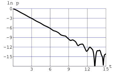
Figure 4: Survival probability as a function of time for $\Delta_{0}=.02$.

For $\Delta=.1$ (see Fig. 5) the FGR regime is seen up to $t=3$.

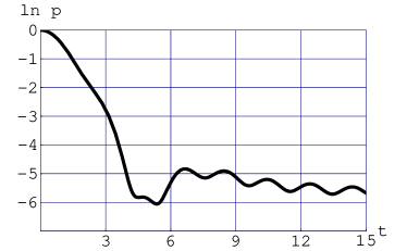
Figure 5: Survival probability as a function of time for $\Delta_{0}=.1$.

For $\Delta_{0}=.2$ (see Fig. 6) the FGR regime is absent.

Figure 6: Survival probability as a function of time for $\Delta_{0}=.2$.

The Rabi oscillations we see already at Fig.5 and still more vividly at Fig.6.

I Dedication

With great pleasure I recall my meetings with I. Vagner and our talks both about physics, and life in general. In addition to being a very good physicist, he also was a very good educator, investing a lot of time and effort in his pedagogical activities. So I would like to dedicate this my modest contribution, mainly of pedagogical nature, to the memory of I. Vagner, who’s untimely death I deeply regret.

References

- (1) U. Fano, Phys. Rev. 124, 1866 (1961).
- (2) G. D. Mahan, Many-Particle Physics, (Plenum Press, New York and London, 1990).
- (3) C. Cohen-Tannoudji, B. Diu, and F. Laloe, Quantum Mechanics, (Wiley, New York, 1977), vol.2, pp. 1344.
- (4) S. Longhi, Phys. Rev. Lett. 97, 110402 (2006).