Entanglement properties in the Inhomogeneous Tavis-Cummings model

Abstract

In this work we study the properties of the atomic entanglement in the eigenstates spectrum of the inhomogeneous Tavis-Cummings Model. The inhomogeneity is present in the coupling among the atoms with quantum electromagnetic field. We calculate analytical expressions for the concurrence and we found that this exhibits a strong dependence on the inhomogeneity.

I Introduction

Quantum correlations have played a central role from the very beginning of Quantum Mechanics, and currently the concept of Entanglement has become a key resource in the research on quantum information and quantum computation Nielsen . The availability of entangled quantum states and their characterization are among the most important questions in quantum information. In this sense, there have been a considerable number of theoretical works that have allowed for characterizing quantum entanglement. From a mathematical point of view, a quantum state of a pair of particles is separable if this can be written as a convex sum of product states werner , $\rho=\sum_{i}^{k}p_{i}|a_{i}\mathbf{\rangle}\left\langle a_{i}\right|\otimes|b_{i}\mathbf{\rangle}\left\langle b_{i}\right|$, where $|a_{i}\mathbf{\rangle}$ and $|b_{i}\mathbf{\rangle}$ correspond to different particles in the pair and $\sum_{i}p_{i}=1$. Actually, separability criteria peres ; horodecki provides us with necessary and sufficient conditions to state if a bipartite quantum state is separable or not. However, these criteria do not allow us to quantify exactly the amount of Entanglement of a given system. Bennet et.al. bennett have characterized the necessary and sufficient channel resources to transmit quantum states. This leads to a measure of entanglement that is called Entanglement of Formation. In other important work, Wootters Hill ; Wootters has shown that the Entanglement of formation of an arbitrary state of two qubits is defined by an exactly calculable quantity called concurrence.

On the other hand, recent advances in the manipulation of collections of atoms have led to the possibility of considering inhomogeneous coupling, for example, in systems of atomic clouds. Some contributions have emerged inspired by this fact. For instance, decoherence of collective atomic states due to the inhomogeneous coupling between the atoms and external fields has been studied by Sun et.al. Sun . Also, Kuzmich et.al. Kuzmich has pointed out the nonsymmetric character of the entanglement of multi-atom quantum states due the inhomogeneity. Recently, decoherence in process of quantum information storage in atomic clouds has been studied Xiong , where the phenomenon of electromagnetically induced transparency (EIT) is present.

Atomic cloud physics could be conveniently described by the Dicke model Dicke , when considering the interaction of atoms with light in free space. The Tavis-Cummings (TC) model Tavis , is suitable when the coupling takes place inside a cavity. In most applications of the TC model, a constant coupling between the atoms and the radiation field is assumed. This simplification is, of course, essential when an analytical description of the coupled system is required cooperativeeffects ; jc1 ; jc2 ; review1 , at least when a small number of atoms is involved. For the case of many atoms, the dynamics can still profit from the associated $SU(2)$ group structure and numerical solutions can be found. However, the situation is drastically different when we consider the more realistic inhomogeneous coupling. In this case, there is no possibility to access the Hilbert space in a simple manner, because all angular momenta representations are mixed along the dynamics and no analytical approach is known.

The entanglement properties of the ground state for the Dicke model has recently been studied by authors in Ref. Orszag ; Ru . In such case, when the coupling between atoms and field is homogeneous, the concurrence between two atoms is independent of the pair considered due to the symmetry of the Dicke states. A similar situation should arise in the case of the Tavis Cummings model. From the point of view of the model properties, it would be interesting to study the quantum correlations between atoms under more general conditions, as is for the case of inhomogeneous coupling. An interesting question to answer would be, how does the spatial profile of the coupling reflect on entanglement between atoms?.

In this work we aim to describe the entanglement properties in the spectrum eigenstates of the TC model Tavis by considering inhomogeneous coupling of the atoms to the quantum electromagnetic field. Specifically we study the bipartite atomic concurrence by tracing out $N-2$ particles. This work is organized as follows: in Sec. II we present the inhomogeneous Tavis-Cummings (ITC) model and the properties of the Hilbert space are shown. In Sec. III, we study the properties of the eigenstates of the model, the bipartite concurrence between atoms is analyzed for different number of excitations in the system. In Sec. IV, we present our concluding remarks.

II The Model

The Hamiltonian describing the inhomogeneous interaction of $N$ atoms with a single mode of a quantum electromagnetic field in the on resonance regime is given by $H=H_{0}+H_{I}$ where

$$H_{0}=a^{{\dagger}}a+S_{z}$$,

,

(1)

besides we have taken $\hbar=1$, $S_{z}=\sum_{j=1}^{N}\sigma_{z}^{j}/2$ and $J_{\pm}=\sum_{j=1}^{N}\kappa_{j}\sigma_{\pm}^{j}$ are the atomic collective operators with $\kappa_{j}=g_{j}/w$. The number of excitation operator $a^{{\dagger}}a+S_{z}$ is an integral of motion for the system Tavis . In addition $\kappa_{j}$ is the inhomogeneous coupling of atoms to the field. In this work, we will consider $\kappa_{j}=\kappa\sin(\pi x_{j}/L)$. We notice that due to the inhomogeneous coupling, the collective atomic operators do not satisfy a closed Lie algebra $su(2)$, leading to a larger total Hilbert space, so that, the description in terms of symmetric Dicke states is not allowed anymore.

An effective approach to study the dynamics of systems with inhomogeneous coupling can be developed lrs . The basic idea of this approach is to follow the Hilbert space that the coupled system will visit along the evolution and to implement a truncation criteria based on a probabilistic argument. In the homogeneous case the eigenstates of $H$ are built as superpositions of eigenstates of $H_{0}$, that is, states with a fixed number of excitations. Thus, the ground state corresponds to the state with all atoms in the lower state. The first excited state corresponds to a superposition of one photon state with all atoms in the ground and the state with zero photons and the symmetric state with one excitation. In the inhomogeneous case we have to find which are the states with a fixed number of excitations. For example, let us consider the state $|n\rangle|\mathbf{\ \bar{0}\rangle}$ where $|n\rangle$ denotes the state with $n$ photons and $|\mathbf{\bar{0}\rangle}$ denotes the collection of $N$ atoms in the ground state $\left|g_{1}g_{2}...g_{N}\right\rangle$. Let us see now how the state $\left|n\right\rangle|\mathbf{\bar{0}\rangle}$ is coupled to other states under the interaction Hamiltonian (1) which conserves the number of excitations. We see that the state $|0\rangle|\mathbf{\bar{0}\rangle}$ is not coupled by the interaction Hamiltonian to other states of the global system, that is,

$$|0\rangle|\mathbf{\bar{0}\rangle\longrightarrow}|0\rangle|\mathbf{\bar{0}\rangle}.$$ (2)

Now, if we have one excitation in the electromagnetic field $|1\rangle|\mathbf{\bar{0}\rangle}$ this state is coupled through the term $J_{+}a$ so that

$$J_{+}a|1\rangle|\mathbf{\bar{0}\rangle=}|0\rangle\sum_{i=1}^{N}\kappa_{i}|\mathbf{\bar{1}}_{i}\mathbf{\rangle}\text{,}$$ (3)

where $|\mathbf{\bar{1}}_{i}\mathbf{\rangle}$ represents the state where the $i$-th atom is excited. We define the normalized state

$$|\mathbf{\bar{1}\rangle=}\frac{1}{\sqrt{\sum_{i=1}^{N}\kappa_{i}^{2}}}\sum_{i=1}^{N}\kappa_{i}|\mathbf{\bar{1}}_{i}\mathbf{\rangle}\text{,}$$ (4)

such that the matrix element of the hamiltonian between $|1\rangle|\mathbf{\bar{0}\rangle}$ and $|0\rangle|\mathbf{\bar{1}\rangle}$ states is given by

$$\langle 0|\langle\mathbf{\bar{1}}|H|1\rangle|\mathbf{\bar{0}\rangle=}\sqrt{\sum_{i=1}^{N}\kappa_{i}^{2}}=N_{1}.$$ (5)

As we can see, the number of excitations is conserved. The resulting state is coupled to the state $|1\rangle|\mathbf{\bar{0}\rangle}$ such that, starting from this root the system evolves in a closed two dimensional subspace $\{|1\rangle|\mathbf{\bar{0}\rangle,}|0\rangle|\mathbf{\bar{1}\rangle}\}$. If we increase the number of excitations $k$ in the system, for example $k=2$, one would expect that the Hilbert space will be spanned by the vectors $\{|2\rangle|\mathbf{\bar{0}\rangle,}|1\rangle|\mathbf{\ \bar{1}\rangle,}|0\rangle|\mathbf{\bar{2}\rangle}\}$, where $|\mathbf{\ \bar{2}\rangle}\mathbf{=}\frac{1}{N_{2}}2\sum_{i<j}\kappa_{i}\kappa_{j}|\mathbf{\bar{2}}_{ij}\mathbf{\rangle}$ and $N_{2}=\sqrt{4\sum_{i<j}\kappa_{i}^{2}\kappa_{j}^{2}}.$ However, it can be shown that the state $|0\rangle|\mathbf{\bar{2}\rangle}$ is coupled through $a^{{\dagger}}J_{-}$ to the state $\left|1\right\rangle\left|\Phi_{1}\right\rangle,$ where $\left|\Phi_{1}\right\rangle=\frac{2}{N_{2}}\sum_{i}(\sum_{j\neq i}\kappa_{i}\kappa_{j}^{2})|\mathbf{\bar{1}}_{i}\mathbf{\rangle}$, which is different from $|\mathbf{\bar{1}\rangle}$, so we can say that $\left|\Phi_{1}\right\rangle$ has a component along $|\mathbf{\bar{1}\rangle}$ and a component along a state $\left|\mathbf{\bar{1}}_{p}\right\rangle$ perpendicular to the state $|\mathbf{\bar{1}\rangle}$ lrs . Thus, if the number of excitations keep growing, then it is possible to generate a sequence of collective atomic states and its respectively perpendicular states as shown by Fig. 1, where the coupling among atomic collective states are shown.

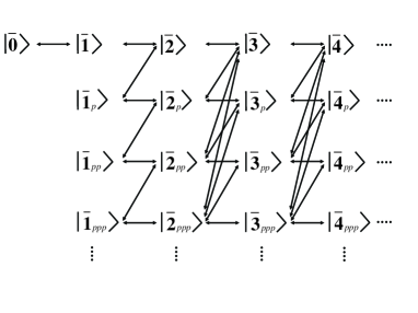
Figure 1: Levels scheme that involve the Hilbert space. Here is possible to see the Hilbert space‘s growth due to the Inhomogeneous coupling.

It is possible to show that the states $\left|\mathbf{\bar{n}}\right\rangle$ (first row in Fig. 1) can be obtained from the repeated application of the operator $aJ_{+}$ over the state $\left|n\right\rangle\left|\mathbf{\bar{0}}\right\rangle$

$$\left(aJ_{+}\right)^{n}\left|n\right\rangle\left|\mathbf{\bar{0}}\right\rangle=\sqrt{n!}\left|0\right\rangle\sum_{i_{1}<i_{2}<..<i_{n}}n!\kappa_{i_{1}}\kappa_{i_{2}}..\kappa_{i_{n}}|\mathbf{\bar{n}}_{i_{1}i_{2}..i_{n}}\mathbf{\rangle},$$ (6)

this implies that the collective atomic states $\left|\mathbf{\bar{n}}\right\rangle$ are given by

$$\left|\mathbf{\bar{n}}\right\rangle=\frac{1}{N_{n}}\sum_{i_{1}<i_{2}<..<i_{n}}n!\kappa_{i_{1}}\kappa_{i_{2}}..\kappa_{i_{n}}|\mathbf{\bar{n}}_{i_{1}i_{2}..i_{n}}\mathbf{\rangle}\text{,}$$ (7)

with $N_{n}^{2}=\sum\limits_{i_{1}<i_{2}<..<i_{n}}\left(n!\right)^{2}\kappa_{i_{1}}^{2}\kappa_{i_{2}}^{2}..\kappa_{i_{n}}^{2}$. On the other hand, the sequence of states $\left|\mathbf{\bar{n}}_{p}\right\rangle$ in the second row of Fig. 1 are given by

$$\left|\mathbf{\bar{n}}_{p}\right\rangle=\frac{1}{\sqrt{\left\langle\Phi_{n}\mid\Phi_{n}\right\rangle-\left|\left\langle\mathbf{\bar{n}}\mid\Phi_{n}\right\rangle\right|^{2}}}\left[\left|\Phi_{n}\right\rangle-\left\langle\mathbf{\bar{n}}\mid\Phi_{n}\right\rangle\left|\mathbf{\bar{n}}\right\rangle\right],$$ (8)

where the states $\left|\Phi_{n}\right\rangle$ are written as

$$\left|\Phi_{n}\right\rangle=(n-1)!\sum_{i_{1}<.....<i_{n}}\kappa_{i_{1}}...\kappa_{i_{n}}\overline{b}_{i_{1}}..._{i_{n}}\left|\mathbf{\bar{n}}_{{}_{i_{1}}..._{i_{n}}}\right\rangle,$$ (9)

and

$$\overline{b}_{i_{1}}..._{i_{n}} = \sum_{\alpha_{1}\neq i_{1}}\kappa_{\alpha_{1}}^{2}+...+\sum_{\alpha_{n}\neq i_{n}}\kappa_{\alpha_{n}}^{2}$$ (10)

$$= \left(N-1\right)\sum_{j=1}^{N}\kappa_{j}^{2}.$$

An accurate description of the model should consider all the states we have found associated with the inhomogeneity. However, based on numerical calculations we have obtained that the spectrum of the Hamiltonian is not sensitive to perpendicular states further than the first row.

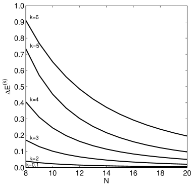
Figure 2: Contribution (%) of second row of Fig. 1 to the energy as a function of the number of atoms $N$. $\Delta E^{\left(k\right)}=100(|(E_{1}^{\left(k\right)}-E_{2}^{\left(k\right)})/E_{1}^{\left(k\right)}|)$, where $E_{1,2}^{\left(k\right)}$ are the energies for $k$ excitations using $1$ or $2$ rows of Fig. 1.

This is shown in Fig. 2, where the effects of the second row on the energies obtained from the first row are quantified. In this figure we observe that the contribution of the second row in Fig. 1 is less than $1\%$. Although the contribution of the second row in Fig. 1 is higher when the number of excitations increases, decreases when the number of atoms is increased, as can be seen in Fig. 2. In other words, the contribution of the second row to the energy, will increase only when $k/N$ increases, where $k$ is the number of excitations. Thus, we can conclude from Fig. 2 that only the first row of Fig. 1 is needed in order to characterize the spectrum of the ITC model for the parameters used in this work. On the other hand, it is important to note that this technique of taking into account only a few rows in Fig. 1 is also valid when the quantum dynamics of the system is studied. In that case the approximation is valid within a given window of time. The size of this window of time will depend on both $N$ and $k$ lrs .

III Eigenstates spectrum properties

In the previous section we have discussed the necessary ingredients to deal with the ITC model. Particulary, we have shown that only a part of the Hilbert space associated to the system is necessary for a suitable description. In this section we study the properties of the eigenstates of the system, by presenting some analytical calculations that allow us to characterize the behavior of the entanglement between a pair of particles. The spectrum and bipartite atomic Concurrence Wootters , can be analytically calculated in the inhomogeneous case for $0,1$ and $2$ excitations respectively. The energies for these cases are given by:

$$\begin{array}[]{l}E^{\left(0\right)}=-\frac{N}{2}\text{,}\\ \lx@intercol\hfil\hfil\lx@intercol\\ E^{\left(1\right)}=1-\frac{N}{2}-N_{1}\text{,}\\ \lx@intercol\hfil\hfil\lx@intercol\\ \lx@intercol\hfil E^{\left(2\right)}=2-\frac{N}{2}-\sqrt{2N_{1}^{2}+\left(N_{2}/N_{1}\right)^{2}}\text{,}\hfil\lx@intercol\end{array}$$ (11)

where $\left(N_{1}\right)^{2}=\sum_{i=1}^{N}\kappa_{i}^{2}$ and $\left(N_{2}\right)^{2}=4\ \sum_{i<j}^{N}\kappa_{i}^{2}\kappa_{j}^{2}$, correspond to the normalization of the states with one and two excitations in Eq. (7) respectively. These energies are associated with the eigenstates

$$\left|\psi^{\left(0\right)}\right\rangle = \left|0\right\rangle\left|\mathbf{\bar{0}}\right\rangle\text{,}$$

$$\left|\psi^{\left(1\right)}\right\rangle = \frac{1}{\sqrt{2}}\left\{\left|1\right\rangle\left|\mathbf{\bar{0}}\right\rangle-\left|0\right\rangle|\mathbf{\bar{1}\rangle}\right\}\text{,}$$ (12)

$$\left|\psi^{\left(2\right)}\right\rangle = \alpha\left|2\right\rangle\left|\mathbf{\bar{0}}\right\rangle-\frac{1}{\sqrt{2}}\left|1\right\rangle|\mathbf{\bar{1}\rangle+}\beta\left|0\right\rangle|\mathbf{\bar{2}\rangle}\text{,}$$

where

$$\alpha=\sqrt{2}\frac{N_{1}^{2}}{\sqrt{4N_{1}^{4}+2N_{2}^{2}}}$$,

.

(13)

From the expressions for eigenstates in Eq. (12) we are able to calculate an analytical expression for the bipartite concurrence of a pair of atoms $i$, $j$ by tracing out respect to the other $N-2$ atoms. For this cases the concurrence is given by:

$$\begin{array}[]{l}C_{ij}^{\left(0\right)}=0,\\ \\ C_{ij}^{\left(1\right)}=\frac{\left|\kappa_{i}\kappa_{j}\right|}{\sum_{i=1}^{N}\kappa_{i}^{2}},\\ \\ C_{ij}^{\left(2\right)}=2\left|\kappa_{i}\kappa_{j}\right|[\frac{1}{2N_{1}^{2}}+\frac{\beta^{2}}{N_{2}^{2}}M_{1}^{2}\\ \text{ \ \ \ \ \ \ \ \ \ \ }-\frac{\beta}{N_{2}}(\alpha^{2}+\frac{1}{2N_{1}^{2}}M_{1}^{2}+\frac{\beta^{2}}{N_{2}^{2}}M_{2}^{2})^{1/2}],\end{array}$$ (14)

with $M_{1}^{2}=\sum_{k\neq i,j}^{N}\kappa_{k}^{2}$, and $M_{2}^{2}=\sum_{m<n\neq i,j}^{N}\kappa_{m}^{2}\kappa_{n}^{2}$.

It is important to note from these expressions for the concurrence that while in the homogeneous TC model the bipartite concurrence of a pair of atoms is independent of the chosen pair, the apparition of inhomogeneity in the coupling between the atoms to the quantum field causes the bipartite concurrence to be dependent on the pair of atoms that we choose. As is apparent from these equations, the entanglement between a pair of atoms is proportional to the coupling constants of atoms to the field. Thus a pair of atoms located in a region of strong coupling to the field will be more entangled. As we will see these dependence of entanglement on the coupling constant appears considering more excitations.

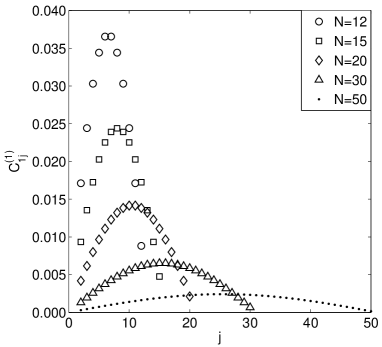
Figure 3: Bipartite concurrence $C_{1,j}$ between the first and the $j$-th atom for $k=1$ excitation for different number of atoms $N$.

Fig. 3 shows the bipartite concurrence $C_{1,j}$, i.e., the concurrence between the first and the $j$-th atom for different total numbers of atoms $N$. All atoms are equally spaced for each case. We observe in this picture the effect of the inhomogeneous coupling of atoms with the field. The concurrence exhibit a reminiscence of the spatial profile of the single mode electromagnetic field. The maximum of entanglement happens for the strongest coupling of the $j$-th atom, which occur for this atom located at the center the cavity. Comparing the entanglement of the first atom with the atom located around the center of the cavity, we realize that as the number of atoms $N$ inside the cavity is increased, entanglement decreases. This is in agreement with that found in the homogeneous case.

In the most general case, the state with $k$ excitations can be written as

$$\left|\Psi^{\left(k\right)}\right\rangle=\sum_{s=0}^{k}A_{s}\left|\mathbf{\bar{s}}\right\rangle_{A}\left|k-s\right\rangle_{F}\text{,}$$ (15)

where $\left|\mathbf{\bar{s}}\right\rangle_{A}$ is the collective atomic state with $s$ excitations defined in Eq. (7) and $A_{s}$ is a coefficient arising from the eigenvalue problem. Tracing out the quantum field, the reduced density matrix for the atomic subsystem is given by

$$\rho^{\left(k\right)}=\sum_{s=0}^{k}\left|A_{s}\right|^{2}\left|\mathbf{\bar{s}}\right\rangle_{A}\left\langle\mathbf{\bar{s}}\right|.$$ (16)

Now, tracing out $N-2$ atoms, the bipartite concurrence between atoms $i,j$  will be given by

$$C_{i,j}^{\left(k\right)} = 2\left|\kappa_{i}\kappa_{j}\right|[\sum_{s=0}^{k}\frac{\left|A_{s}\right|^{2}}{N_{s}^{2}}M_{s-1}^{2}$$ (17)

$$-[\sum_{s,s^{\prime}=0}^{k}\frac{\left|A_{s}\right|^{2}\left|A_{s^{\prime}}\right|^{2}}{N_{s}^{2}N_{s^{\prime}}^{2}}M_{s-2}^{2}M_{s^{\prime}}^{2}]^{1/2}],$$

where we have defined

$$N_{p}=\sqrt{\sum\limits_{n_{1}<n_{2}<..<n_{p}}\left(n!\right)^{2}\kappa_{n_{1}}^{2}\kappa_{n_{2}}^{2}..\kappa_{n_{p}}^{2}}$$,

.

(18)

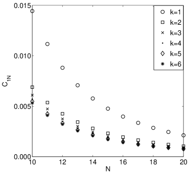
Figure 4: Bipartite concurrence $C_{1N}$ between the first and the last atom for $k=1,2,...,6$ excitations as a function of the number of atoms $N$.

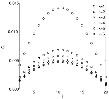
Figure 5: Bipartite concurrence $C_{1,j}$ between the first and the $j$-th atom for $k=1,2,...,6$ excitations with $N=20$ atoms.

As we can see in the general expression for the concurrence (17) for $k$ excitations and $N$ atoms, the entanglement between two of these atoms still depends directly on the coupling constant. As shown by this result this is one important feature of entanglement that the TC model exhibit for the inhomogeneous case. This makes the difference with the the situation for the homogeneous case where only depends on the total number of atoms $N$ for a given number of excitations $k$ Orszag . Fig. 4 shows the concurrence between the first atom and the last atom as a function of the number of atoms inside the cavity. In this picture we can observe how the concurrence decreased when the number of total excitations $k$ in the system increases. However, when $N\gg 1$ the concurrence becomes less dependent on the number of excitations tending to a fixed value. Fig. 5, as Fig. 3 shows the concurrence $C_{1,j}$ between the first and the $j$-th atom in the cavity. The effects of the inhomogeneous coupling and the loss of entanglement when the number of excitation is increased are also clear in this figure.

IV Summary

In the present work we have found that although the symmetry $SU(2)$ no longer exits in the ITC model and consequently a treatment in terms of symmetric Dicke states is not feasible, there are still some features that can be analyzed. In particular, the bipartite concurrence of the eigenstates of the model can be obtained exhibiting an explicit dependence on the inhomogeneity in addition to the dependence on the number of atoms and the number of excitations.

- (1) M. A. Nielsen, I. L. Chuang, ”Quantum Computation and Quantum Information” Cambridge University Press (2000).
- (2) Reinhard F. Werner, Phys. Rev. A 40, 4277 (1989).
- (3) A. Peres, Phys. Rev. Lett. 77, 1413 (1996).
- (4) M. Horodecki, P. Horodecki, R. Horodecki, Phys. Lett. A 223, 1 (1996).
- (5) C. H. Bennett, G. Brassard, S. Popescu, B. Schumacher, J. A. Smolin, W. K. Wootters Phys.Rev.Lett. 76,722-725 (1996); C. H. Bennett, D. P. DiVincenzo, J. A. Smolin, W. K. Wootters, Phys.Rev. A, 54 3824-3851(1996)
- (6) Scott Hill and William K. Wootters, Phys. Rev. Lett. 78, 5022 (1997).
- (7) William K. Wootters, Phys. Rev. Lett. 80, 2245 (1998).
- (8) C. P. Sun, S. Yi and L. You, Phys. Rev. A 67, 063815 (2003).
- (9) A. Kuzmich and T. A. B. Kennedy, Phys. Rev. Lett. 92, 030407 (2004).
- (10) Xiong-Jun Liu et al, Phys. Rev. A 73, 013825 (2006).
- (11) R. H. Dicke, Phys. Rev. 93, 99 (1954).
- (12) M. Tavis and F.W. Cummings, Phys. Rev. 170, 379 (1967).
- (13) M. Orzag, R. Ramírez, J.C. Retamal, and C. Saavedra, Phys Rev. A 49, 2933 (1994).
- (14) C. Saavedra, A.B. Klimov, S.M. Chumakov and J.C. Retamal, Phys. Rev. A 58, 4078 (1998).
- (15) J.C. Retamal, C. Saavedra, A.B. Klimov and S.M. Chumakov, Phys. Rev. A 55, 2413 (1997).
- (16) B. W. Shore and P. L. Knight, J. Mod. Opt. 40, 1195 (1993).
- (17) V. Bužec, M. Orszag, and M. Roško, Phys. Rev. Lett. 94, 163601 (2005).
- (18) Ru-Fen Liu, and Chia-Chu Chen, quant-ph/0510071.
- (19) C. E. López, H. Christ, J. C. Retamal and E. Solano, quant-ph/0610078.