Optimal computation with non-unitary quantum walks

Abstract

Quantum versions of random walks on the line and the cycle show a quadratic improvement over classical random walks in their spreading rates and mixing times respectively. Non-unitary quantum walks can provide a useful optimisation of these properties, producing a more uniform distribution on the line, and faster mixing times on the cycle. We investigate the interplay between quantum and random dynamics by comparing the resources required, and examining numerically how the level of quantum correlations varies during the walk. We show numerically that the optimal non-unitary quantum walk proceeds such that the quantum correlations are nearly all removed at the point of the final measurement. This requires only $O(\log T)$ random bits for a quantum walk of $T$ steps.

,

1 Introduction

Quantum computing has produced a range of algorithms showing improvements over classical algorithms, among the most celebrated are Grover’s search of an unsorted database [1] and Shor’s algorithm for factoring large numbers [2]. In the search for new quantum algorithms, quantum versions of Markov chains are a natural place to look, since classical Markov chains provide the basis for some of the best known algorithms for hard problems such as approximating the permanent of a matrix [3] and $k$SAT (with $k>2$) [4].

Simple quantum generalisations of classical random walks spread quadratically faster on the line [6, 5], and mix quadratically faster on the cycle [7]. These promising early results were soon followed by several algorithms based on quantum walks. Shenvi et al [8] proved a quantum walk can solve the unsorted database search problem quadratically faster, and Childs et al [9] proved an exponential speed up for crossing a particular type of graph. Ambainis [10] gives an overview of quantum walk algorithms, and Kempe [11] provides an introductory review of quantum walks and their properties.

Quantum walks on simple one-dimensional structures remain a fertile testing ground for further research. It was shown numerically by Kendon and Tregenna [12] and recently proved by Richter [13, 14] that the addition of random noise or measurements to the quantum walk dynamics can optimise the spreading and mixing properties for quantum walks on both the line and the cycle. A detailed survey of the effects of such decoherence in quantum walks can be found in [15]. In this paper we examine how the interplay between quantum evolution and random noise or measurements produces optimal computational properties. The paper is organised as follows. In §2 we describe the basic quantum walk model we used for this study, and in §3 we extend this model to include non-unitary operations. We then outline how to count both quantum and random computational resources in a comparable way in §4. Section 5 introduces the measure of quantum correlations we are using, the negativity. In §6 we present our results for the quantum walk on the line, and in §7 our results for the walk on the cycle. Discussion and conclusions are given in §8.

2 Quantum walks on the line and the cycle

This study considers quantum walks taking place in discrete time and space, using a quantum coin to control the choice of direction. This is because we measure how “quantum” the walk is by examining the correlations between the quantum coin and the quantum walker. A different method for assessing “quantumness” would be needed for continuous-time quantum walks (introduced for quantum algorithms by Farhi and Gutmann [16]).

A discrete-time (coined) quantum walk dynamics consists of a quantum “coin toss” operation $\mathbf{C}$, followed by a shift operation $\mathbf{S}$ to move the quantum walker to a new position. These are repeated alternately for $T$ steps of the quantum walk, and the final position of the quantum walker is measured. For quantum walks on the line and the cycle, we have just two choices of which way to step, so the quantum coin is two-sided. We write $|x,c\rangle$ for a quantum walker at position $x$ with a coin in state $c\in\{+1,-1\}$. For a walk on the line, $x\in\mathbb{Z}$ and for a walk on a cycle of size $N$, we have $x\in\mathbb{Z}_{N}$. A classical random walk can only occupy one location at any given time, but a quantum walker can be in a superposition of different locations. The full state of the quantum walk $|\Psi(t)\rangle$ can be written as a combination of terms in each basis state $|x,c\rangle$,

$$|\Psi(t)\rangle=\sum_{x,c}\psi_{x,c}(t)|x,c\rangle,$$ (1)

where $\psi_{x,c}(t)\in\mathbb{C}$. By convention, the normalisation is defined to be

$$\sum_{x,c}|\psi_{x,c}(t)|^{2}=1.$$ (2)

When the quantum walk is measured (in the basis just defined), the walker is found in a single location with a definite coin state, but we cannot predict with certainty which state this will be, it could be any of the states in the superposition described by eq. (1). The probability of finding the quantum walker at position $y$ with the coin in state $b$ is given by

$$P(y,b,t)=|\langle y,b|\Psi(t)\rangle|^{2}=|\psi_{y,b}(t)|^{2}$$ (3)

since the basis states are orthogonal, $\langle y,b|x,c\rangle=\delta_{xy}\delta_{bc}$.

The coin toss and shift operators can be defined in terms of their action on the basis states $|x,c\rangle$,

$$\mathbf{S}|x,c\rangle=|x+c,c\rangle$$ (4)

$$\mathbf{C}|x,c\rangle=(|x,-c\rangle+c|x,c\rangle)/\sqrt{2}$$ (5)

One can add more general bias or phase into the coin toss operation, see, for example, [17], but this does not greatly change the basic properties of the quantum walk on a line or cycle, so we will consider only the unbiased case in this paper. For a quantum walk starting at position $x=0$ with the coin in a superposition state $(|{-1}\rangle+i|{+1}\rangle)/\sqrt{2}$, (where $i=\sqrt{-1}$) we can write a quantum walk of $T$ steps as

$$|\Psi(T)\rangle=(\mathbf{SC})^{T}(|0,-1\rangle+i|0,+1\rangle)/\sqrt{2}$$ (6)

The solution for $|\Psi(T)\rangle$ may be obtained by various methods such as Fourier analysis [5] and path counting [6], and has been studied extensively. The key result is that spreading on the line proceeds linearly with the number of time steps. We can use the standard deviation $\sigma_{Q}(T)$ of the probability distribution to quantify the spreading rate. For a quantum walk on the line,

$$\sigma_{Q}(T)=\sum_{x,c}x^{2}P(x,c,T)\simeq\left(1-\frac{1}{\sqrt{2}}\right)^{1/2}T,$$ (7)

asymptotically in the limit of large $T$. In contrast, for the classical random walk, the standard deviation is $\sigma_{C}(T)=\sqrt{T}$.

On the cycle, we are interested in mixing times rather than spreading. Mixing times can be defined in a number of different ways, we choose the definition given in [7],

$$M(\epsilon)=\min\left\{T\enspace|\enspace\forall\enspace t>T:||P(x,t)-P_{u}||_{\text{tv}}<\epsilon\right\}$$ (8)

where $P_{u}$ is the limiting distribution over the cycle, and the total variational distance (TVD) is defined as

$$||P(x,T)-P_{u}||_{\text{tv}}\equiv\sum_{x}|P(x,T)-P_{u}|.$$ (9)

A classical random walk on the cycle mixes to within $\epsilon$ of the uniform distribution in time proportional to $N^{2}\log(1/\epsilon)$, where $\epsilon$ can be chosen arbitrarily small.

Pure quantum walks, on the other hand, do not mix to a stationary distribution. Their deterministic dynamics ensures they continue to oscillate indefinitely. There are several ways to obtain mixing behaviour, first explored by Aharonov et al [7]. By defining a time-averaged probability distribution for the quantum walk,

$$\overline{P(x,c,T)}=\frac{1}{T}\sum_{t=0}^{T-1}P(x,c,t)$$ (10)

they proved that $\overline{P(x,c,T)}$ does converge to a stationary distribution on a cycle, and that on odd-sized cycles the stationary distribution is uniform. A mixing time can be defined for $\overline{P(x,c,T)}$,

$$\overline{M}(\epsilon)=\min\left\{T\enspace|\enspace\forall\enspace t>T:||\overline{P(x,t)}-P_{u}||_{\text{tv}}<\epsilon\right\}.$$ (11)

and Aharonov et al [7] proved that, for odd-sized cycles, $\overline{M}(\epsilon)$ is bounded above by $O(\epsilon^{-3}N\log N)$, almost quadratically faster (in $N$) than a classical random walk. Kendon and Tregenna [12], observed numerically that $\overline{M}(\epsilon)\sim O(N/\epsilon)$, this has been recently confirmed analytically by Richter [14].

Notice that we pay a price for our time-averaging: the scaling with the precision $\epsilon$ is now linear instead of logarithmic. Aharonov et al [7] provide a fix for this in the form of a “warm start”. The quantum walk is run several times, each repetition starting from the final state of the previous run. A small number of such repetitions is sufficient to reduce the scaling of the mixing time $\overline{M}(\epsilon)$ to logarithmic in $\epsilon$.

Both the quantum walk on the line and the cycle thus provide a quadratic speed up over classical random walks. This quadratic speed up does not carry over to all quantum walks on higher dimensional structures, see, for example, [18, 19, 20]. It remains an open question how ubiquitous this behaviour really is.

3 Non-unitary quantum walks

The quantum walk dynamics described in the previous section is a pure quantum evolution terminated by a final measurement to determine the outcome of the quantum walk. If, instead, the quantum walk is measured after every step, it is easy to see that it becomes a classical random walk. In between these two extremes, a smaller number of measurements can be included in the quantum walk dynamics, as in the “warm start” already mentioned for the walk on the cycle. This is not a new idea. Quantum walks with measurements were first explored in [21] for controlling a physical quantum walk in an atom optical system.

We are thus led to define a more general quantum walk by including the possibility of non-unitary operations at each step (pure quantum dynamics is unitary, measurements are non-unitary). Kendon and Sanders [22] provide a general formulation of non-unitary quantum walks using superoperators. We will not need the full generality here, we restrict this study to randomly-occurring uncorrelated non-unitary events, and measurements at specific chosen times during the quantum walk. Nonetheless, the evolution of the quantum walk must now be described using a density operator $\bm{\rho}(t)$ given by

$$\bm{\rho}(t+1)=(1-p)\mathbf{SC}\bm{\rho}(t)\mathbf{C}^{{\dagger}}\mathbf{S}^{{\dagger}}+p\sum_{j}\mathbb{P}_{j}\mathbf{SC}\bm{\rho}(t)\mathbf{C}^{{\dagger}}\mathbf{S}^{{\dagger}}\mathbb{P}_{j}^{{\dagger}}.$$ (12)

Here $\mathbb{P}_{j}$ is a projection that represents the action of the non-unitary operator and $p$ is the probability of applying this operator per time step, or, completely equivalent mathematically, to a weak coupling between the quantum walk system and a Markovian environment with coupling strength $p$. For a pure state, the density operator $\bm{\rho}(t)\equiv|\Psi(t)\rangle\langle\Psi(t)|$, it thus has the normalisation $\rm{Tr}[\bm{\rho}(t)]=1$.

Full analytical solution of a non-unitary quantum walk has been done only for a few instances. For quantum walks on the line, Brun et al [23] analysed the case of random measurements on the coin only. While analytical solution is challenging, eq. (12) lends itself readily to numerical simulation since $\bm{\rho}$, $\mathbf{S}$ and $\mathbf{C}$ can be manipulated as complex matrices, while the $\mathbb{P}_{j}$ generally remove some or all of the off-diagonal entries in $\bm{\rho}$. Kendon and Tregenna [12] evolved eq. (12) numerically for various choices of $\mathbb{P}_{j}$, projection onto the position space, projection into the coin space in the preferred basis ($|\pm 1\rangle$), and projection of both coin and position. In all cases, the spreading rate is reduced, in the long time limit [23], it becomes proportional to $\sqrt{T}$ instead of proportional to $T$. More interesting behaviour is seen for intermediate times and noise rates $p$ with noise applied to the position. Kendon and Tregenna observed that, for $2\lesssim pT\lesssim 5$, the distribution becomes very close to uniform while retaining the full quantum linear spreading rate [12]. With noise applied to the coin only, the distribution retains a cusp shape. To quantify this the TVD given by eq. (9) is used, this time with $P_{u}$ defined to be a top-hat of appropriate width $x\in\{\pm T/\sqrt{2}\}$, see [5, 6].

For a quantum walk on the cycle subjected to Markovian noise, the mixing behaviour is dramatically improved, provided noise is applied to the position. The noise guarantees mixing to the uniform distribution, and a similar judicious choice of $2\lesssim pN\lesssim 5$ produces the minimum mixing time [12]. Noise on the coin only does cause the quantum walk on a cycle to mix, but not significantly faster than a classical random walk. Furthermore, the time-averaging is no longer needed, fast mixing occurs in time $O(N\log(1/\epsilon)$, as shown in numerical work by Maloyer and Kendon [15, 24], and recently proved by Richter [14]. Significantly, Richter also proved that the randomness produced by quantum measurements alone is sufficient to produce an optimal mixing time. By applying measurements at regular intervals, instead of randomly with probability $p$, the speed up is still obtained.

We thus have two examples where the optimal computational properties are obtained for a judicious combination of quantum dynamics and measurements, which introduce a component of randomness into the otherwise deterministic quantum dynamics. In order to understand more about how this mixture of quantum and random resources combine to produce their computational power, we next describe how we can compare them in the quantum walk.

4 Comparing quantum and classical computational resources

Our goal is to compare the resources required to perform a quantum walk with those required for a classical random walk, to find out which is more efficient when the random resources are taken into account as well as the memory and gate operations. What we will find is that the optimal non-unitary quantum walk on the line run for $T$ steps requires only $O(\log T)$ extra quantum gates and ancillae compared with a pure quantum walk. Since the pure quantum walk uses $O(T\log T)$ quantum gates and $O(\log T)$ qubits, the extra resource costs are insignificant to leading order. A classical random walk producing the same computational outcome requires $T^{2}$ steps. This can be accomplished using $O(T^{2}\log T)$ quantum gates and $O(T^{2})$ ancillae. The extra resources compared with a fully quantum walk are mainly needed to generate the random bits. Applying the same reasoning to the optimal quantum walk on a cycle shows that it is similarly efficient. We now explain in detail how these results are obtained.

We can quantify the randomness added to, or generated by, the non-unitary quantum walk by counting up the number of random bits, either supplied to time the random measurements, or produced from the results of those measurements and then used as input to the next iteration of the quantum walk. The quantum resources can be quantified by counting the number of gate operations required, in a similar manner to classical computational complexity. What we then need is a way to compare the quantum and random resources.

We first observe that, if we have only quantum resources to hand, we can generate random bits by using a quantum gate followed by a measurement. To illustrate, using a quantum coin by itself, we apply the coin toss then measure. For example,

$$\mathbf{C}|{+1\rangle}=\{|{-1}\rangle+|{+1}\rangle\}/\sqrt{2}.$$ (13)

The measurement outcome is $|{-1}\rangle$ 50% of the time, and $|{+1}\rangle$ the other 50% of the time, i.e. one random bit. We can repeat this procedure (starting with the coin in whichever state was obtained after measuring) to obtain further random bits. Of course, the converse does not work: if we have only classical random bits, we cannot efficiently simulate all the properties of a general quantum system. What is notable is that a quantum computer comes with randomness as a “built in” function, whereas classical computation does not and it must be added separately, or faked (pseudo-randomness) at some significant computational cost.

An alternative way of viewing non-unitary quantum evolution is as a pure quantum evolution in a larger system that includes an ancilla or environment degrees of freedom. Let us illustrate this with the quantum coin in an arbitrary state

$$|\Psi_{c}\rangle=\alpha|{-1}\rangle-\beta|{+1}\rangle.$$ (14)

If we measure in the computational basis, we find the coin in state $|{-1}\rangle$ with probability $\alpha^{2}$ and in state $|{+1}\rangle$ with probability $\beta^{2}$. Now we add an ancilla qubit, another two state system with states $|e_{0}\rangle$ and $|e_{1}\rangle$. We start with the ancilla in state $|e_{0}\rangle$ and apply a CNOT gate with the quantum coin as the control and the ancilla as the target,

$$\text{CNOT}|\Psi_{c}\rangle|e_{0}\rangle=\alpha|{-1}\rangle|e_{0}\rangle-\beta|{+1}\rangle|e_{1}\rangle.$$ (15)

Now we discard the ancilla, and consider the state of the quantum coin only. Mathematically, we trace out the ancilla, leaving

$$\text{Tr}_{e}\left[\alpha|{-1}\rangle|e_{0}\rangle-\beta|{+1}\rangle|e_{1}\rangle\right]=\alpha^{2}|{-1}\rangle\langle{-1}|+\beta^{2}|{+1}\rangle\langle{+1}|.$$ (16)

This is now a mixed state with classical probabilities that match the probabilities measured in the quantum state eq. (14). However, it now has no useful quantum properties. Notice in particular that the phase ($-\beta$ rather than $+\beta$) is lost from the original superposition state. The quantum phases are crucial for generating the computational speed up in a quantum walk, via the cancellations (interference) they produce when the quantum walk arrives at the same location via two different paths. Kendon and Sanders [22] employ this method of measuring the quantum coin with a more general coupling to explore the effects of weak measurements.

Based on these examples, we can see that one way to count resources in a non-unitary quantum walk is to count them all as quantum resources. We count the number of quantum gates, and we also tally up the number of quantum bits (qubits) we require, including the ancillae that we use in the measurement process. A random bit thus requires one quantum gate, and one qubit ancilla to couple to the qubit being measured. Note that we cannot “recycle” the ancillae, since returning them to a pure quantum state $|e_{0}\rangle$ would require further operations and ancillae.

We next apply the quantum resource counting to the quantum walk on the line, run for $T$ steps with non-unitary noise rate $p$. This is equivalent to including a total of $pT$ measurements at random intervals during our quantum walk. Since the noise can be applied as a weak coupling at every step, we do not need to generate random numbers to decide when to apply the measurements. Each step of the quantum walk uses two quantum gates, $\mathbf{C}$ and $\mathbf{S}$. Now, $\mathbf{C}$ acts non-trivially on the coin qubit only, but $\mathbf{S}$ acts on the whole quantum walk system. We assume the position of the quantum walker is encoded in a quantum register of size $\lceil\log(2T+1)\rceil$ qubits. Thus $\mathbf{S}$ will need to consist of $O(\log T)$ elementary gates each acting on one or two qubits. Next we turn to the noise. There are two cases we need to consider: noise acting on the coin only, and noise acting on the position space as well. (Noise acting on both the position and coin differs only $O(1)$ in resources required from noise acting on the position only, so we will consider these two cases as one.) We have already noted that noise on the coin only does not have the same computational effect as noise acting on the position. We will now see that the required resources are different. The $pT$ random measurements applied to the coin only require $O(pT)$ quantum gates, and $O(pT)$ ancillae. Applying noise to the position requires $O(pT\log T)$ quantum gates and $O(pT\log T)$ ancillae. These random bits are, of course, drawn from the distribution of the quantum walk on the line, which is not uniformly random, so this estimate is an upper bound on the true minimum required. The number of qubits we need for the quantum walk is one for the coin plus $\lceil\log(2T+1)\rceil$ for the position. We thus require a total of
coin noise position noise quantum gates: $O(T\log T+pT)$ $O(T\log T+pT\log T)$ qubits: $O(\log T+pT)$ $O(\log T+pT\log T)$

Let us check the extreme cases, pure quantum and fully classical. For the pure quantum walk (no noise or randomness) we have $p=0$, so for large $T$ we require $O(T\log T)$ quantum gates and $O(\log T)$ qubits. For the classical random walk, $p=1$ corresponding to measurements applied at every step, but it is sufficient to apply measurements to the coin only, so we find we still require $O(T\log T)$ quantum gates, but we need an additional $T$ ancillae to generate the randomness at each step. However, to make a fair comparison in terms of the outcome of the walks, the classical random walk must run for longer. To achieve the same spreading as a quantum walk run for $T$ steps, we require $\sim T^{2}/2$ steps of a classical random walk, requiring $O(T^{2}\log T)$ quantum gates and $O(T^{2})$ ancillae. Viewed from this perspective, randomness is an expensive resource! Of course, what we did not count is the cost of maintaining the quantum coherences necessary for the pure quantum walk to function properly. However, this depends on the particular physical implementation of a quantum computer. While there is no fundamental minimum requirement that we know of, in practice we expect the costs of maintaining coherence in a realistic quantum computer to be very high in terms of the quantum error correction overhead that will be required [25].

Finally we are ready to consider the optimal quantum walk. As already noted, the closest to uniform distribution requires measurements to be applied to the position, and is obtained for a noise rate such that $pT\sim O(1)$. Our resource requirements under this condition are $O(T\log T+\log T)$ quantum gates and $O((1+O(1))\log T)$ qubits. We thus need to add only $O(\log T)$ extra quantum gates and ancillae, to optimise the quantum walk, a small increase in the resources compared to the total resources required for the pure quantum walk.

We can do the same comparisons for the non-unitary quantum walk on the cycle. To obtain a distribution within $\epsilon$ of the uniform distribution on a cycle of size $N$, we run for $M(\epsilon)$ steps with noise rate rate $p$.
coin noise position noise quantum gates: $O(M(\epsilon)\log N+pM(\epsilon))$ $O(M(\epsilon)\log N+pM(\epsilon)\log N)$ qubits: $O(\log N+pM(\epsilon))$ $O(\log N+pM(\epsilon)\log N)$

For the time-averaged mixing time $\overline{M(\epsilon)}$, we need to add $O(\log\overline{M(\epsilon)})$ gates and qubits, to choose a random time at which to stop between $0\dots T$, as per the definitions in eqs. (10) and (11).

Using $M(\epsilon)\sim O(N\log(1/\epsilon))$ for the quantum walk with noise rate $p$ such that $pN\sim O(1)$, and $M(\epsilon)\sim O(N^{2}\log(1/\epsilon))$ for a classical random walk, we can compare the resources required in each case. Noise on the coin applied at every step ($p=1$) is sufficient to produce a classical random walk, which thus requires $O(N^{2}\log N\log(1/\epsilon))$ quantum gates and $O(N^{2}\log(1/\epsilon))$ qubits. For the optimal quantum walk we consider only noise on the position, since noise on the coin only does not allow the quantum walk to mix significantly faster than a classical random walk [12]. A pure quantum walk run for $N\log(1/\epsilon)$ steps (which does not mix) requires $O(N\log N\log(1/\epsilon))$ quantum gates and $O(\log N)$ qubits. For optimal mixing we need to add $O(\log N\log(1/\epsilon))$ quantum gates and qubits. Again, only a small amount of randomness is required to optimise the quantum walk on a cycle, while the cost for the classical random walk is much higher.

5 Entanglement in mixed states

Having estimated the number of quantum gates required for the quantum walk, it would be interesting to know whether they are actually used to full effect. The unitary operations that generate quantum correlations are not guaranteed to do so every time they are applied. Depending on the current state of the system, they can just as easily remove correlations as add them. So, we will look directly at the quantum correlations in the quantum walk system by calculating the entanglement between the coin and the position of the quantum walker. We choose our entanglement measure to be the negativity because this can be calculated numerically in a fairly straightforward manner for density operators such as $\bm{\rho}(t)$, and there are few options that meet this criterion. This is not ideal. The negativity does not relate directly to information-theoretic quantities, like entropy, that could be compared with the number of random bits, but it will suffice for our purposes in this study.

The negativity is defined as follows. First we must choose a division of our system into two (or more) subsystems between which to identify the entanglement. For our quantum walk, the natural division is between the coin and the quantum walker’s position. We note that the entanglement across this division will be the same whether we regard the quantum walk as a qubit coin and a unary position, or as the position encoded in a binary quantum register (because the Hilbert spaces are the same size). We perform a partial transpose on one subsystem to obtain a new matrix $\bm{\rho}^{\prime}(t)$. For example, the partial transpose with respect to the coin subsystem is

$$\rho^{\prime}_{xc,yb}(t)=\rho_{xb,yc}(t)$$ (17)

where $x$, $y$ are position indices and $c$, $b$ are coin state indices. Next, we determine the spectrum of $\bm{\rho}^{\prime}(t)$, denoted by$\{\lambda^{\prime}_{i}\}$. The normalisation of $\bm{\rho}(t)$ is carried over to $\bm{\rho}^{\prime}(t)$, so $\sum_{i}\lambda^{\prime}_{i}=1$, but unlike $\bm{\rho}(t)$, it is possible for $\bm{\rho}^{\prime}(t)$ to have negative eigenvalues. The negativity is defined [26, 27, 28] as

$$E=\frac{1}{2}\left(\sum_{i}|\lambda^{\prime}_{i}|-1\right),$$ (18)

which is just the sum of the negative eigenvalues. The negativity ranges between zero and one, with any non-zero value indicating entanglement is present. If the negativity is zero, it means the state is probably not entangled, but there can be exceptions [29]. The exceptions are known to be relatively rare in the set of all possible states [30], and the entanglement they contain is difficult to apply to useful quantum tasks [29]. For this study, we will not need the fine-grained detail of these possible exceptions.

6 Entanglement in a quantum walk on the line

The entanglement in a pure state quantum walk has been studied previously, see for example, [31]. It fluctuates with each step, and eventually settles down to an asymptotic value that depends on the initial state of the quantum coin, and on any bias in the quantum coin operator $\mathbf{C}$. The addition of noise smooths out this behaviour, see

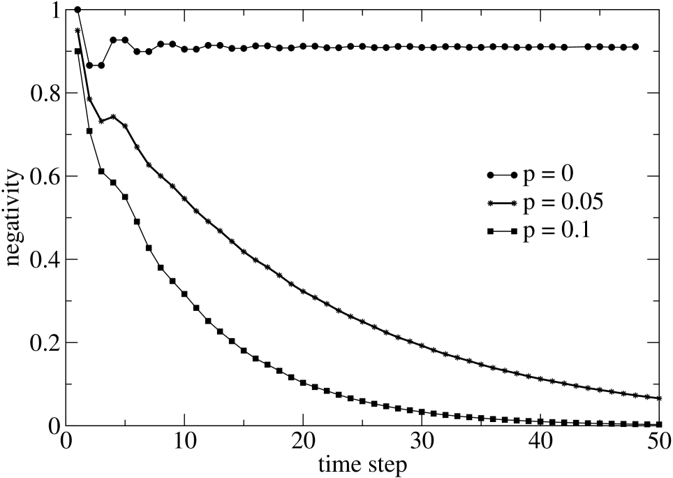
Figure 1: Negativity for noise rate $p=0$ (circles), $p=0.05$ (asterisks) and $p=0.1$ (squares) for a quantum walk on the line with noise applied to both coin and position, run for 50 time steps.

fig. 1, and steadily reduces the level of entanglement between the coin and the position. Recall that a noise rate $p$ can be interpreted as a weak measurement of strength $p$ applied every step, or, a full measurement applied only with probability $p$, whereupon the steady reduction in entanglement can be regarded as the average effect of a few random measurements. Our simulations simply take eq. (12) and evolve it numerically, calculating the negativity and TVD using an appropriate top hat distribution, for various types of noise and noise rate $p$.

Guided by the results in [12] and [31], we focused on the entanglement at the end of the quantum walk, just before the final measurement, and considered how it varies as the noise rate $p$ is varied. We examined three cases of noise, applying it to both the coin and position, and also separately to just the coin or the position. An example is shown in fig. 2.

Figure 2: Negativity (diamonds) and TVD for noise applied to position (dashed), coin (dotted) and both (solid) for a quantum walk on the line of 100 steps.

Both the TVD from the optimal top hat distribution, and the negativity are plotted. The minimum in the TVD indicates the optimal measurement rate $p$. For a quantum walk of 100 steps the optimal $p$ ranges through $0.025\lesssim p\lesssim 0.05$. Note that the minimum for measurements on the coin only is much shallower. The distribution in this case retains a cusp shape [12]. The negativity also remains above zero for longer than when noise is applied to the position of the walker, indicating the coin measurements are less effective at removing the quantum correlations. If noise is applied to the position, with or without noise on the coin as well, the negativity drops to zero at $p\simeq 0.055$, shortly after the optimal noise rate is reached. The optimal amount of randomness is thus just about the amount required to remove all the the quantum correlations from the system. This make intuitive sense: we are trying to achieve a uniform distribution on the line, in which any location within the top hat region is equally likely. Quantum correlations distort this smooth distribution, giving it peaks and troughs, especially at the ends of the top hat [5, 6]. If the noise rate is turned up until the classical random walk is obtained for $p=1$, classical correlations build up to produce the binomial distribution in which the quantum walker is more likely to be found nearer the starting point of the walk.

7 Entanglement in a quantum walk on cycles

For the mixing time on cycles, there are extra considerations. The mixing time in general depends not only on the size of the cycle, but also on how close to uniform one sets the threshold $\epsilon$. As already noted, pure quantum walks don’t mix unless something is done to disrupt the pure quantum evolution, and random or even regular repeated measurements efficiently change the behaviour into that of fast mixing to the uniform distribution. Note also that the optimal rate of measurement $2\lesssim pN\lesssim 5$ is independent of the threshold $\epsilon$, even though the main effect is to provide logarithmic scaling of the mixing time with $\epsilon$.

We studied how the entanglement varies during the quantum walk on a cycle, with the noise rate $p$ chosen to be near-optimal. As with the walk on the line, we examined the three cases of noise applied to both the position and coin, and applied to just the position or coin separately. Again noise applied to the coin only does not provide a significant improvement in the behaviour compared with noise applied to the position. The results for a typical example, a cycle of size $N=29$ with noise applied to the position only, are shown in fig. 3.

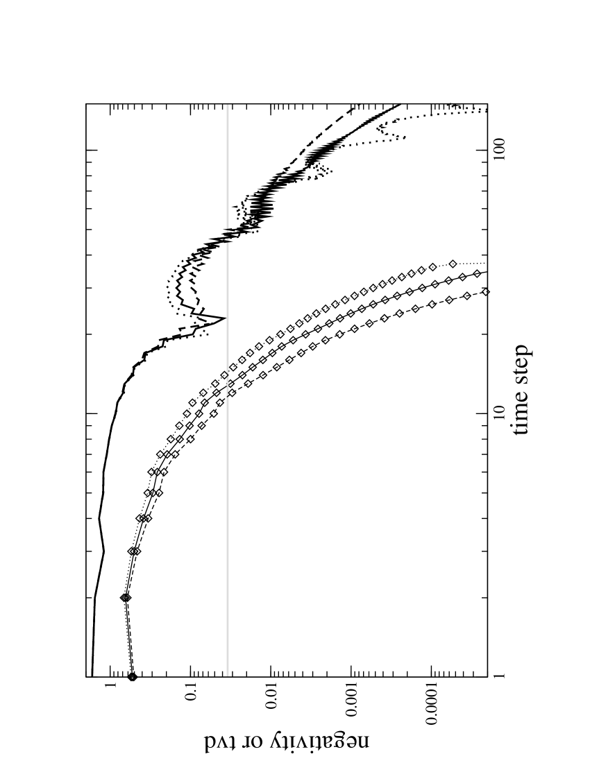
Figure 3: Negativity (diamonds) and TVD for noise applied to position for a quantum walk on the cycle of size 29 with $p=0.2239$ (dotted), $p=0.2511$ (solid) and $p=0.2818$ (dashed). The grey horizontal line is at $1/29$.

While the actual mixing time is determined by the choice of $\epsilon$, we have indicated the position of $1/N$ in fig. 3, this being the probability of finding the walker at one location in a uniform distribution. The time at which the TVD drops below this line is around the time the entanglement also drops to zero. The variability of the TVD shows that the mixing time is not a smooth function of $\epsilon$, so we cannot expect to determine a more precise result. As we argued for the walk on the line, quantum correlations are incompatible with the result we want, a uniform distribution, so the optimal quantum walk arranges for the quantum correlations to be removed by the end of the process.

8 Discussion

The optimal quantum walk on the line and cycle is a carefully balanced combination of quantum dynamics with randomness provided by repeated measurements during the evolution of the walk. We have shown that, while the quantum correlations are necessary to obtain linear spreading and mixing times, they must be neutralised to produce a uniform final distribution. We have also analysed the resources required for a non-unitary quantum walk and shown that the additional randomness required to obtain the optimal behaviour is only logarithmic in the size of the problem. Since a quantum computer has randomness as a built in function, this is a very efficient use of resources compared to performing a classical random walk, which requires an amount of randomness quadratic in the size of the problem.

While the relationship between quantum entanglement and shared randomness is well-studied in quantum communications theory, for example, see [32], the relationship between the two types of resources in quantum computation has received little attention. The idea of combining measurements with quantum gates is well-established [33], but little is known about the importance of each contribution to the power of the computational process. Note in particular that in the cluster state model, random measurement outcomes are corrected, requiring extra computational steps, whereas the non-unitary quantum walk takes advantage of this randomness to enhance the computational efficiency. Our results contribute to the task of quantifying this relationship and to furthering our understanding of how to harness the computational power of quantum systems.

We thank many people for interesting discussions of quantum walks, among them, Ivens Carneiro, Hilary Carteret, Jochen Endrejat, Barbara Kraus, Peter Richter, Barry Sanders, Mario Szegedy, and Tino Tamon stimulated our thinking for the work in this paper. VK is funded by a Royal Society University Research Fellowship.

References

- [1] L. K. Grover, Quantum mechanics helps in searching for a needle in a haystack, Phys. Rev. Lett. 79 (1997) 325.
- [2] P. W. Shor, Polynomial-time algorithms for prime factorization and discrete logarithms on a quantum computer, SIAM J. Sci Statist. Comput. 26 (1997) 1484.
- [3] M. Jerrum, A. Sinclair, E. Vigoda, A polynomial-time approximation algorithm for the permanent of a matrix with non-negative entries, in: Proc. 33rd Annual ACM STOC, ACM, NY, 2001, pp. 712–721.
- [4] U. Schöning, A probabilistic algorithm for k-SAT and constraint satisfaction problems, in: 40th Annual Symposium on FOCS, IEEE, Los Alamitos, CA, 1999, pp. 17–19.
- [5] A. Nayak, A. Vishwanath, Quantum walk on the line, extended abstract, ArXiv: quant-ph/0010117 (2000).
- [6] A. Ambainis, E. Bach, A. Nayak, A. Vishwanath, J. Watrous, One-dimensional quantum walks, in: Proc. 33rd Annual ACM STOC, ACM, NY, 2001, pp. 60–69.
- [7] Aharonov, D, A. Ambainis, J. Kempe, U. Vazirani, Quantum walks on graphs, in: Proc. 33rd Annual ACM STOC, ACM, NY, 2001, pp. 50–59.
- [8] N. Shenvi, J. Kempe, K. Birgitta Whaley, A quantum random walk search algorithm, Phys. Rev. A 67 (2003) 052307.
- [9] A. M. Childs, R. Cleve, E. Deotto, E. Farhi, S. Gutmann, D. A. Spielman, Exponential algorithmic speedup by a quantum walk, in: Proc. 35th Annual ACM STOC, ACM, NY, 2003, pp. 59–68.
- [10] A. Ambainis, Quantum walk algorithms for element distinctness, in: 45th Annual IEEE Symposium on Foundations of Computer Science, Oct 17-19, 2004, IEEE Computer Society Press, Los Alamitos, CA, 2004, pp. 22–31.
- [11] J. Kempe, Quantum random walk algorithms, Contemp. Phys. 44 (3) (2003) 302–327.
- [12] V. Kendon, B. Tregenna, Decoherence can be useful in quantum walks, Phys. Rev. A 67 (2003) 042315.
- [13] P. Richter, Almost uniform sampling in quantum walks, New J. Phys. 9 (2007) 72.
- [14] P. Richter, Quantum speedup of classical mixing processes, ArXiv: quant-ph/0609204 (2006).
- [15] V. Kendon, Decoherence in quantum walks – a review., Math. Struct. in Comp. Sci. To appear. ArXiv: quant-ph/0606016.
- [16] E. Farhi, S. Gutmann, Quantum computation and decison trees, Phys. Rev. A 58 (1998) 915–928.
- [17] E. Bach, S. Coppersmith, M. P. Goldschen, R. Joynt, J. Watrous, One-dimensional quantum walks with absorbing boundaries, J. Comput. Syst. Sci. 69 (4) (2004) 562–592.
- [18] T. D. Mackay, S. D. Bartlett, L. T. Stephenson, B. C. Sanders, Quantum walks in higher dimensions, J. Phys. A: Math. Gen. 35 (2002) 2745.
- [19] B. Tregenna, W. Flanagan, R. Maile, V. Kendon, Controlling discrete quantum walks: coins and initial states, New J. Phys. 5 (2003) 83.
- [20] H. Krovi, T. A. Brun, Quantum walks with infinite hitting times, Phys. Rev. A 74 (4) (2006) 042334.
- [21] Aharonov, Y, L. Davidovich, N. Zagury, Quantum random walks, Phys. Rev. A 48 (2) (1992) 1687–1690.
- [22] V. M. Kendon, B. C. Sanders, Complementarity and quantum walks, Phys. Rev. A 71 (2004) 022307.
- [23] T. A. Brun, H. A. Carteret, A. Ambainis, Quantum random walks with decoherent coins, Phys. Rev. A 67 (2003) 032304.
- [24] O. Maloyer, V. Kendon, Decoherence vs entanglement in coined quantum walks (2007).
- [25] D. Gottesman, A theory of fault-tolerant quantum computation, Phys. Rev. A 57 (1998) 127.
- [26] A. Peres, Separability criterion for density matrices, Phys. Rev. Lett. 77 (1996) 1413–1415.
- [27] M. Horodecki, P. Horodecki, R. Horodecki, Separability of mixed states: necessary and sufficient conditions, Phys. Lett. A 223 (1996) 1.
- [28] G. Vidal, R. F. Werner, A computable measure of entanglement, Phys. Rev. A 65 (2002) 032314.
- [29] M. Horodecki, P. Horodecki, R. Horodecki, Mixed-state entanglement and distillation: is there a “bound” entanglement in nature?, Phys. Rev. Lett. 80 (1998) 5239–5242.
- [30] K. Życzkowski, On the volume of the set of mixed entangled states II, Phys. Rev. A 60 (1999) 3496–3507.
- [31] I. Carneiro, M. Loo, X. Xu, M. Girerd, V. M. Kendon, P. L. Knight, Entanglement in coined quantum walks on regular graphs, New J. Phys. 7 (2005) 56, ArXiv: quant-ph/0504042.
- [32] C. H. Bennett, P. W. Shor, J. A. Smolin, A. V. Thapliyal, Entanglement-assisted capacity of a quantum channel and the reverse Shannon theorem, IEEE Trans. on Info. Theory 48 (10) (2002) 2637–2655.
- [33] R. Jozsa, An introduction to measurement based quantum computation, ArXiv: quant-ph/0508124 (2005).