Quantum Mechanical Reflection Resonances

Abstract

Resonances in the reflection probability amplitude $r(E)$ can occur in energy ranges in which the reflection probability $R(E)=|r(E)|^{2}$ is 1. They occur as the phase $\phi(E)$ defined by $r(E)=t^{*}(E)/t(E)=1e^{i2\phi(E)}$ undergoes a rapid change of $\pi$ radians. During this transition the phase angle exhibits a Lorentzian profile in that $d\phi(E)/dE\simeq 1/[(E-E_{0})^{2}+(\hbar\gamma/2)^{2}]$. The energy $E_{0}$ identifies the location of a quasi-bound state, $\gamma$ measures the lifetime of this state, and $t(E)$ is a matrix element of the transfer operator. Methods for computing and measuring these resonances are proposed.

I Introduction

Quantum mechanical transmission resonances, as observed for example in the Ramsauer effect, have been known for a long time Bohm51 . At a transmission resonance the reflection probability is small, and may even be zero if the potential satisfies specific properties. Conversely, if the transmission probability is small the reflection probability will be large.

There is a large class of potentials for which the transmission probability is zero and therefore the reflection probability is one in certain energy ranges. In one dimension these potentials have unequal asymptotic values on the left and right, with $V_{L}<E<V_{R}$. Here $V_{L}$ ($V_{R}$) is the asymptotic potential on the left (right) and $E$ is the energy of a particle, incident from the left. One such potential is shown in Fig. 1. This is a washboard potential, commonly encountered with biased Josephson junctions Roberto . Particles incident from the left with energy $-10<E<19.1eV$ will be reflected with 100% probability, so that $R(E)=|r(E)|^{2}=1.0$. It is the purpose of this work to show that the reflection probability amplitude $r(E)$ undergoes resonances in the sense that the reflection phase shift $\phi(E)$, defined by $r(E)=1e^{i2\phi(E)}$, undergoes rapid phase shifts when the incident energy sweeps through a narrow energy range. These resonances correspond to energies at which quasistable states occur in the potential. The sharp resonances can be described by a Lorentzian line shape whose peak locates the energy of the metastable state and whose width is determined by the lifetime of the state.

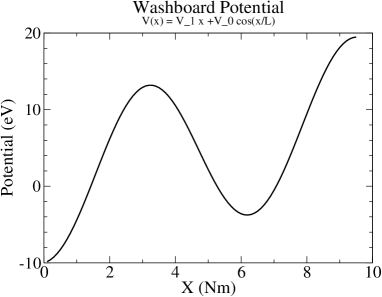
Figure 1: Washboard potential: $V(x)=V_{0}\cos(x/L)+V_{1}x$, with $V_{0}=-10$ eV, $V_{1}=1$ eV, $L=1$ Nm, $0<x<9.7$ Nm, and $V_{L}=-10$ eV, $V_{R}=19.9$ eV. ${\cal H}=P^{2}/2M+V(x)$, $M=100m_{e}$. This potential has two metastable states, at $E=0.32$ eV and $E=7.87$ eV.

II Hamiltonian

We choose as hamiltonian

$${\cal H}=\frac{P^{2}}{2m}+V(\gamma)=\frac{P^{2}}{2M}+V_{0}\cos(\gamma)+V_{1}\gamma$$ (1)

Washboard potentials of this type are typically found in biased Josephson junctions Roberto . In such cases the coordinate $\gamma$ is the phase difference across the junction, $P$ is the canonically conjugate momentum, $M=C_{J}\hbar^{2}/4e^{2}$ is expressed in terms of the junction capacitance $C_{J}$ and fundamental constants $e$ and $\hbar$, $V_{0}$ is the Josephson energy, and $V_{1}/V_{0}=I/I_{c}$, where $I$ is the bias current and $I_{c}$ is the critical current. For simplicity, we will interpret this hamiltonian as describing a particle of mass $M=100m_{e}$ with coordinate $x=\gamma L$ in the potential whose parameters are as described in the caption of Fig. 1.

III Reflection Phase

The phase shift can be computed by constructing the transfer matrix for the potential. This relates the input and output amplitudes on the left with those on the right (the notation is as used in Gil04 ):

$$\left[\begin{array}[]{c}A_{L}\\ B_{L}\end{array}\right]=\left[\begin{array}[]{cc}t_{11}(E)&t_{12}(E)\\ t_{21}(E)&t_{22}(E)\end{array}\right]\left[\begin{array}[]{c}A_{R}\\ B_{R}\end{array}\right]$$ (2)

The reflection amplitude is $r(E)=t_{21}(E)/t_{11}(E)$. For reflecting boundary conditions these two matrix elements are complex conjugates of each other:

$$t_{21}(E)=t_{11}(E)^{*}~{}~{}~{}~{}~{}~{}~{}~{}~{}t_{11}(E)=a(E)+ib(E)$$ (3)

In the neighborhood of a metastable state the the matrix element $t_{11}(E)$ has the form $e^{-i\theta}[(E-E_{0})-i(\hbar\gamma/2)]$, where the rapidly varying phase $\tan^{-1}\left(\hbar\gamma/2/(E-E_{0})\right)$ rides on top of a slowly varying $\theta(E)$. The total phase is $\phi(E)=\theta(E)+\tan^{-1}\left((\hbar\gamma/2)/(E-E_{0})\right)$. From this we immediately derive a Lorentzian line shape:

$$\frac{d\phi(E)}{dE}-\frac{d\theta(E)}{dE}=\frac{(\hbar\gamma/2)}{(E-E_{0})^{2}+(\hbar\gamma/2)^{2}}$$ (4)

When $\theta(E)$ is slowly varying over the narrow range of a resonance, the term $d\theta/dE$ can be neglected and $d\phi(E)/dE$ shows a Lorentzian lineshape.

The real and imaginary parts of the matrix element $t_{11}(E)$ have been computed for the potential shown in Fig. 1. They are plotted in the neighborhood of the first excited resonance at $E=+7.87$ eV in Fig. 2. The phase shift $\phi(E)$ computed from the real and imaginary parts of $t_{11}(E)$ are shown in Fig. 3.

The real and imaginary parts of these matrix elements can be written in the form

$$\begin{array}[]{rcl}a(E)&=&\alpha(E)(E-E_{r})\\ b(E)&=&\beta(E)(E-E_{i})\end{array}$$ (5)

They have zero crossings at $E_{r}$ and $E_{i}$: the sharper the resonance, the closer the crossings. The slopes $\alpha(E)$ and $\beta(E)$ are related to $\cos(\theta)$ and $\sin(\theta)$. Generally the slopes are only weakly dependent on $E$. When this is the case

$$\begin{array}[]{c}|t_{11}(E)|^{2}=|t_{21}(E)|^{2}=a(E)^{2}+b(E)^{2}=\\ \\ (\alpha^{2}+\beta^{2})[(E-E_{0})^{2}+(\hbar\gamma/2)^{2}]\end{array}$$ (6)

Its inverse has a Lorentzian shape

$$\frac{1}{|t_{11}(E)|^{2}}=\frac{\rm cst}{(E-E_{0})^{2}+(\hbar\gamma/2)^{2}}$$ (7)

The center $E_{0}$ and halfwidth $\hbar\gamma/2$ of the peak are weighted averages of the zero crossings of the real and imaginary parts of $t_{11}(E)$:

$$E_{0}=\frac{\alpha^{2}E_{r}+\beta^{2}E_{i}}{\alpha^{2}+\beta^{2}}~{}~{}~{}~{}~{}~{}~{}~{}\hbar\gamma/2=\frac{|\alpha\beta(E_{r}-E_{i})|}{\alpha^{2}+\beta^{2}}$$ (8)

Figure 4 plots the Lorentzian $1/|t_{11}(E)|^{2}$ in the neighborhood of a sharp resonance for the washboard potential. Also plotted is the inverse of this function, which should be a simple parabola if the peak does in fact have a Lorentzian profile. When the slowly varying part of $\phi(E)$ is removed, so that $\phi(E)$ varies rapidly through $\pi$ radians as $E$ passes the resonance, a plot of $d\phi(E)/dE$ vs. $E$ produces a Lorentzian line shape centered at the resonance. The plots of $1/|t_{11}(E)|^{2}$ and $d\phi(E)/dE$ are indistinguishable.

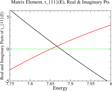
Figure 2: Real (negative slope) and imaginary (positive slope) parts $a(E)$ and $b(E)$ of the matrix element $t_{11}(E)=a(E)+ib(E)$.

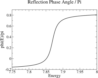
Figure 3: Phase shift $\phi(E)/\pi$ computed from the real and imaginary parts of the matrix element $t_{11}(E)$.

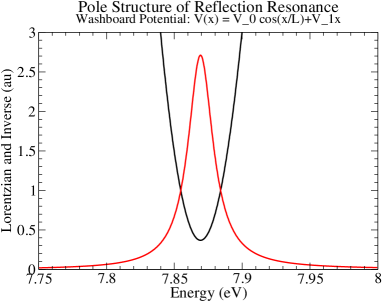
Figure 4: Reflection resonance for the washboard potential shown in Fig. 1. Also shown is its inverse, which should be a simple parabola if the resonance is a Lorentzian.

IV Physical Interpretation

Rapid phase changes in transmission and/or reflection amplitudes are associated with the existence of metastable states. They have also received a nice interpretation by Wigner as time delays caused by these resonances wigner . That is, as a particle enters a region where a metastable state can exist, it undergoes multiple internal reflections before exiting this region. These internal reflections are responsible for the prolonged time delay before transmission or reflection. The Wigner time delay is measured quantitatively by $\delta t=\hbar d\phi/dE$. This delay time has been studied under scattering conditions 96 , reflecting boundary conditions 97 , and metastable escape conditions 98 ; 99 .

The phase shift calculated in Sect. III shows Lorentzian peaks near resonances riding on top of a slowly varying background. The slowly varying background is due to the slight time delay for the reflected particle due to the longer distance it must travel before reaching the classically forbidden region. The fast variation is the excess time delay spent in the well near the energy of the metastable (resonant) state.

V Differential Spectroscopy

It may not always be easy to extract phase information from reflection amplitudes. An alternative method for locating reflection resonances would therefore be useful. One such method is illustrated in Fig. 5. This is a schematic for a Differential Reflection Resonance Spectrometer. A beam of thermal electrons ($E\simeq 0$ eV) is incident on a beam splitter from arm 0 of the interferometer. The beam is split into arms 1 and 2. Each of these beams is reflected off identical washboard potentials. The two reflecting potentials are biased at voltages $-V$ and $-V-\delta V$ Gil04 . The separation $\delta V$ between the two biasing potentials is chosen small, of the order of 10 profile halfwidths. The potential $V$ is scanned through the resonance, and the intensity profile of the interfering beams in arm 3 is recorded. The split beams undergo rapid $2\pi$ phase shifts approximately $\delta V$ apart. As these two phase shifts occur the output intensity undergoes a rapid symmetric variation as shown in Fig. 6. The symmetry of this pattern and the separation of the rapidly fluctuating features by $\delta V$ is a clear indication that a reflection resonance exists approximately where the first feature undergoes its most rapid variation. This result is insensitive to amplitude and phase inequalities in the two returning beams due to different arm lengths and unequal splitting in the beam splitter.

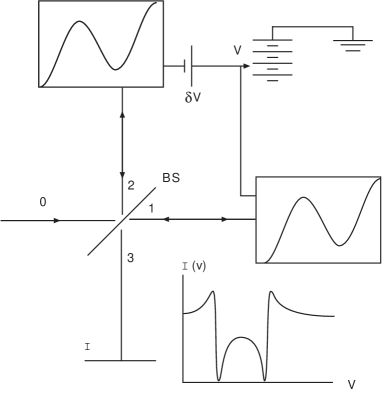
Figure 5: Reflection resonance interferometer. A beam of thermal electrons $E\simeq 0$ is incident on a beamsplitter. The two resulting beams are reflected off identical washboard potentials that are biased at $-V$ and $-V-\delta V$, with $\delta V$ of the order of 10 halfwidths of the resonant peak. The bias potential $V$ is scanned through the resonance and the intensity of the recombined beam in the output arm is monitored.

VI Lorentz Profiles from Intensities

Line shape information can be extracted from intensity information. The total amplitude of the signal in the measurement arm of the interferometer is

$$A(V)=a_{1}e^{i\alpha_{1}}r_{1}(V)+a_{2}e^{i\alpha_{2}}r_{2}(V+\delta V)$$ (9)

Here $r_{1}(V)=e^{i2\phi(V)}$ is the reflection amplitude for particles reflected from the potential biased at $V$ in arm 1, and similarly for $r_{2}(V+\delta V)=e^{i2\phi(V+\delta V)}$ in arm 2. The returning beams are weighted with complex amplitudes $a_{i}e^{i\alpha_{i}}$, with $a_{i}>0$. The amplitudes $a_{i}$ are typically unequal due to nonperfect beam splitting, and the difference in the angles $\alpha_{i}$ is related to differences in arm lengths. The observed intensity is

$$\begin{array}[]{c}I(V)=|A(V)|^{2}=a_{1}^{2}+a_{2}^{2}+\\ \\ 2a_{1}a_{2}\cos\left[(\alpha_{1}-\alpha_{2})+2(\phi(V)-\phi(V+\delta V))\right]\end{array}$$ (10)

A typical intensity profile is shown in Fig. 6. For this pattern $\delta V=0.2eV$, $a_{1}=1,\alpha_{1}=0$ and $a_{2}=0.7,\alpha=0.2\times 2\pi$. The intensity varies between $I_{\rm Max}$ and $I_{\rm min}$, where $\cos\left[*\right]$ assumes values $+1$ and $-1$. Several features of this profile are worth mentioning. (1) The pattern is symmetric about the midpoint $V+\frac{1}{2}\delta V$. This comes about because the intensity is a function of the difference $2(\phi(V)-\phi(V+\delta V))$, and these two functions are identical except for the energy shift. Outside the range of rapid variation this difference is zero, while on transiting the resonance region the difference changes from 0 to $2\pi$ radians, then back down to 0. (2) The pattern has five critical points. The two critical points near the resonance at $-V=-7.9$ eV occur as $2\phi(V)$ changes through $2\pi$ radians and the two critial points near $-V-\delta V$ occur as $2\phi(V+\delta V)$ changes through $2\pi$ radians. The fifth critical point, at the symmetry point $V+\frac{1}{2}\delta V$, is due to the overlap of the shoulders of the two Lorentzians centered near $V=-7.9$ eV and $V=-8.1$ eV, as will be shown shortly.

The derivative of the intensity is

$$\begin{array}[]{c}\displaystyle\frac{dI}{dV}=-2a_{1}a_{2}\sin\left[(\alpha_{1}-\alpha_{2})+2(\phi(V)-\phi(V+\delta V))\right]\\ \\ \displaystyle\times 2\left(\frac{d\phi(V)}{dV}-\frac{d\phi(V+\delta V)}{dV}\right)\end{array}$$ (11)

At $I_{\rm Max}$ and $I_{\rm min}$ where $\cos\left[*\right]=\pm 1$, $\sin\left[*\right]$ passes through zero. As a result $2a_{1}a_{2}\sin\left[*\right]=\pm\sqrt{(I_{\rm Max}-I)(I-I_{\rm min})}$. Therefore, the intensity data can be processed according to

$$\pm\frac{dI(V)/dV}{\sqrt{(I_{\rm Max}-I)(I-I_{\rm min})}}=2\left(\frac{d\phi(V)}{dV}-\frac{d\phi(V+\delta V)}{dV}\right)$$ (12)

The right hand side is the difference of two Lorentzians. This difference vanishes at the midpoint $V+\frac{1}{2}\delta V$, where the falling shoulder of the Lorentian around the resonance near $-7.9$ eV is equal to the negative of the rising shoulder of the displaced resonance near $-8.1$ eV (fifth critical point of $dI(V)/dV$). The expression on the left of Equ.(11) is difficult to compute near the critical points where $I=I_{\rm Max}$ or $I_{\rm min}$. In these regions the intensity should be approximated in second order, and the singular expression simplifies to $\sqrt{|d^{2}I(V)/dV^{2}|}{\sqrt{(I_{\rm Max}-I_{\rm min})/2}}$. The absolute value of the right hand side of Equ.(11) is plotted in Fig. 7 for the intensity data shown in Fig. 6. The absolute value consists of two Lorentzian profiles, one surrounding the resonance near $-7.9$ eV, the other around the displaced resonance near $-8.1$ eV. These two peaks are displaced vertically from the curve $dI(V)/dV$, shown below it.

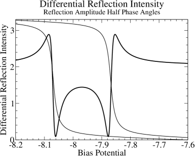
Figure 6: Intensity in the output arm as a function of biasing voltage $V$ in the Differential Reflection Resonance Spectroscopy setup shown in Fig. 5 (darker curve). For this simulation we used $\delta V=0.2$ eV, $r_{1}=e^{i2\phi(V)}$ and $r_{2}=ae^{i\theta}e^{i2\phi(V+\delta V)}$ with $a=0.7$ and $\theta=0.2\times 2\pi$. The plots of $\phi(V)$ and $\phi(V+\delta V)$ are shown in lighter curves after being shifted down by an equal phase.

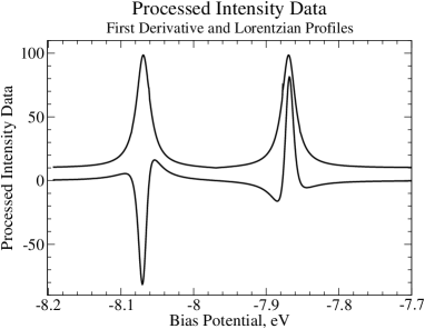
Figure 7: Plot of $dI/dV$ for the intensity shown in Fig. 6. Vertically offset: plot of the function $dI/dV/\sqrt{(I_{\rm Max}-I)(I-I_{\rm min})}$, showing recovery of two Lorentzian line profiles at the appropriate biasing potentials.

VII Conclusions

For scattering potentials possessing bound states, the phase of the matrix element $t_{11}(E)$ increases by $\pi$ radians each time $E$ increases through a bound state value (real pole of the $S$-matrix) and increases rapidly through $\pi$ radians each time $E$ passes through a transmission resonance. For such resonances the transmission line shape $1/|t_{11}(E)|^{2}$ is well approximated by a Lorentzian. For reflecting potentials of the type discussed here (c.f., Fig. 1), the reflection amplitude $r(E)=t_{11}(E)^{*}/t_{11}(E)$ increases rapidly through $2\pi$ radians each time $E$ passes through a reflection resonance. For such resonances the line shape $1/|t_{11}(E)|^{2}$ is well approximated by a Lorentzian. The Lorentzian can be computed from the real and imaginary parts of the appropriate transfer or scattering matrix element (c.f., Equ.(5) and Fig. 4). It can also be computed as $d\phi(E)/dE$ (c.f., Fig. 3). We have described how this information can be extracted from unique intensity signatures obtained from a Differential Reflection Resonance Interferometer (c.f., Equ. (11) and Figs. 6 and 7). Quasibound states in washboard potentials are currently located experimentally by spectroscopic methods Roberto . This requires at least one of the states to be occupied. The method proposed here provides a completely different approach for locating such states. Further, the states need not be occupied.

References

- (1) D. Bohm, Quantum Theory, Englewood Cliffs, NJ: Prentice Hall, 1951.
- (2) P. R. Johnson, F. W. Strauch, A. J. Dragt, R. C. Ramos, C. J. Lobb, J. R. Anderson, and F. C. Wellstood, Phys. Rev. B67, 020509(R), (2003).
- (3) R. Gilmore, Elementary Quantum Mechanics in One Dimension, Baltimore: The Johns Hopkins University Press, 2004.
- (4) E. P. Wigner, Phys. Rev. 98, 145 (1955).
- (5) V. A. Gopar, P. A. Mello, and M. Büttiker, Phys. Rev. Lett. 77, 3005 (1996).
- (6) A. Comtet and C. Texier, J. Phys. A: Math. Gen. 30, 8017 (1997).
- (7) G. N. Gibson, G. Dunne, and K. J. Bergquist, Phys. Rev. Lett. 81, 2663 (1998).
- (8) E. Y. Sidky and I. Ben-Itzhak, Phys. Rev. A60, 3586 (1999).