We report on a search for mutually unbiased bases (MUBs) in 6 dimensions. We find only triplets of MUBs, and thus do not come close to the theoretical upper bound 7. However, we point out that the natural habitat for sets of MUBs is the set of all complex Hadamard matrices of the given order, and we introduce a natural notion of distance between bases in Hilbert space. This allows us to draw a detailed map of where in the landscape the MUB triplets are situated. We use available tools, such as the theory of the discrete Fourier transform, to organise our results. Finally we present some evidence for the conjecture that there exists a four dimensional family of complex Hadamard matrices of order 6. If this conjecture is true the landscape in which one may search for MUBs is much larger than previously thought.

ingemar@physto.se, wojtek@gorce.if.uj.edu.pl, asae@physto.se,

jalar@mai.liu.se, wtadej@wp.pl, karol@tatry.if.uj.edu.pl

1. Introduction

This is a paper on 6 by 6 matrices. Its scope would therefore seem rather limited, but we will address two much discussed open problems. The first concerns the classification of complex Hadamard matrices, and the second the existence (or not) of complete sets of mutually unbiased bases. These problems are connected to each other, they are of considerable interest in quantum information theory, and they have a long history. The study of complex Hadamard matrices was begun by Sylvester [1], and by Hadamard himself [2], while the second problem has appeared (in various guises) in quantum theory [3, 4], operator algebra theory [5], Lie algebra theory [6], and elsewhere [7, 8]. It would seem as if all questions concerning single digit dimensions should have been settled by now, but this is not the case.

A complex Hadamard matrix is, by definition, a unitary matrix all of whose matrix elements have equal modulus. Much of the mathematical literature concerns the special case of real Hadamard matrices, but from now on we will take “Hadamard matrix” to refer to a complex Hadamard matrix. An obvious question concerns the classification of all $N\times N$ Hadamard matrices. It has been settled for $N\leq 5$ [9], but for all larger values of $N$ it is open [10, 11].

The columns of a unitary matrix define an orthonormal basis in Hilbert space. The basis defined by an Hadamard matrix has the property that the modulus of the scalar product between any one of its vectors and any vector in the standard basis (whose vectors has only one non-zero entry) is always equal to $1/\sqrt{N}$. Again by definition, we say that these two bases are mutually unbiased, or MUB for short. One can now ask how many bases, with all pairs being MUB with respect to each other, one can find in a Hilbert space of a given dimension $N$. It is known that there can be at most $N+1$ MUBs, and when $N$ is the power of a prime number the answer is $N+1$ [4]. For other values of $N$ the question is open. For $N=6$, all that is known is that the number of MUBs is at least 3 and at most 7 [12].

The set of Hadamard matrices provides a landscape where sets of MUBs live. In fact classifying the set of Hadamard matrices is equivalent to classifying the set of ordered MUB pairs, up to natural equivalences [13]. Once such a classification has been carried out we proceed to list all MUB triplets, all MUB quartets (if any), and so on. However, let us admit at the outset that we have carried through this strategy only piecemeal—and for $N=6$ we did not find any MUB quartets.

In section 2 of this paper we describe the known Hadamard matrices of order 6, and sort out some problems concerning equivalences between them. In section 3 we recall some facts about MUBs, and decide when sets of MUBs should be regarded as equivalent. In section 4 we define a useful notion of distance between orthonormal bases. The distance attains its maximum when the bases are unbiased. In section 5 we describe a search for all MUBs whose vectors are composed of rational roots of unity of some modest orders; the most interesting of our choices is the 24th root. In section 6 we describe the set of all bases that are MUB with respect to both the standard and the Fourier bases [14], and show how this set can be understood from properties of the discrete Fourier transform. In section 7 we describe MUBs of a related type, where the Hadamard matrices have a particular block structure. Finally, in section 8 we give some arguments suggesting that there exists a four dimensional family of Hadamard matrices—the largest known family has two dimensions only. Readers interested in Hadamard matrices only can skip sections 3-7, but our main contention is that readers interested in MUBs should skip nothing. Section 9 states some conclusions.

Notation: $z$ is a complex number, and $\bar{z}$ its complex conjugate. The rational root of unity $e^{2\pi i/n}$ is denoted $\omega$. Its integer powers are called $n$th roots. A special case is $q=e^{2\pi i/N}$, where $N$ is the dimension of the Hilbert space. A matrix element of the matrix $M$ is denoted $M_{ab}$, $M^{\rm T}$ is the transposed matrix, and $M^{\dagger}$ is the adjoint. The index $a$ usually runs from $0$ to $5$.

2. Complex Hadamard matrices

According to our definition an Hadamard matrix $H$ is a unitary matrix whose matrix elements obey

$$|H_{ab}|^{2}=\frac{1}{N}\ ,\hskip 22.76219pt0\leq a,b\leq N-1\ .$$ (1)

An example that exists for all $N$ is the Fourier matrix ${\bf F}$, whose matrix elements are

$$F_{ab}=\frac{1}{\sqrt{N}}q^{ab}\ ,\hskip 22.76219ptq\equiv e^{2\pi i/N}\ .$$ (2)

Two Hadamard matrices $H_{1}$ and $H_{2}$ are called equivalent [9], written $H_{1}\approx H_{2}$, if there exist diagonal unitary matrices $D_{1}$ and $D_{2}$ and permutation matrices $P_{1}$ and $P_{2}$ such that

$$H_{1}=D_{1}P_{1}\cdot H_{2}\cdot P_{2}D_{2}\ .$$ (3)

That is to say, we are allowed to rephase and permute rows as well as columns. This is an equivalence relation, and we are interested in classifying all the equivalence classes for a given matrix size $N$.

We will usually present our Hadamard matrices in dephased form, which means that all elements in the first row and the first column are real and positive. This can always be achieved using diagonal unitaries, but it does not fix the equivalence class completely. If the Hadamard matrix is written in any other form it is said to be enphased.

For $N=2$, $3$, and $5$, the Fourier matrix is unique, in the sense that it represents the only equivalence class of Hadamard matrices [9]. For $N=4$ there exists a one parameter family of equivalence classes, including the Fourier matrix as well as a real Hadamard matrix [2]. This family exhausts the set of equivalence classes when $N=4$. Let us remark that continuous families appear also when $N=7$ [11], so that their existence does not hinge on $N$ not being a prime number.

We will print concrete Hadamards matrices in boldface. When $N=6$ the following representatives of different equivalence classes are known to us:

• A two parameter family ${\bf F}(x_{1},x_{2})$, including the Fourier matrix ${\bf F}(0,0)$.

• The transpose ${\bf F}^{\rm T}(x_{1},x_{2})$ of the above.

• A circulant matrix ${\bf C}$ found by Björck [16], and its complex conjugate.

• A one parameter family ${\bf D}(x)$, including a matrix ${\bf D}$ composed of fourth roots of unity, called Diţă’s matrix [10].

• A one parameter family ${\bf B}(\theta)$ that interpolates between ${\bf C}$ and ${\bf D}$ [17].

• Tao’s matrix ${\bf S}$, composed of third roots of unity [18, 19].

Attribution may be difficult; the Diţă family, or representatives thereof, was discovered several times [20, 9, 12]. With one exception, namely the family ${\bf B}(\theta)$, the known continuous families are of the special kind called affine families [11], which means that some of the matrix elements can be multiplied with free phase factors in such a way that the matrix remains Hadamard.

We now go through the items in our list. The Fourier family is explicitly

$${\bf F}(x_{1},x_{2})=\left[\begin{array}[]{cccccc}1&1&1&1&1&1\\ 1&qz_{1}&q^{2}z_{2}&q^{3}&q^{4}z_{1}&q^{5}z_{2}\\ 1&q^{2}&q^{4}&1&q^{2}&q^{4}\\ 1&q^{3}z_{1}&z_{2}&q^{3}&z_{1}&q^{3}z_{2}\\ 1&q^{4}&q^{2}&1&q^{4}&q^{2}\\ 1&q^{5}z_{1}&q^{4}z_{2}&q^{3}&q^{2}z_{1}&qz_{2}\end{array}\right]\ ,\hskip 14.22636pt\begin{array}[]{l}z_{1}\equiv e^{2\pi ix_{1}}\\ \\ \\ z_{2}\equiv e^{2\pi ix_{2}}\end{array}\ .$$ (4)

The two free parameters arise essentially because a six dimensional space can be written as a tensor product; see section 7. This is an affine family, since there are no restrictions on the phase factors $z_{1}$ and $z_{2}$.

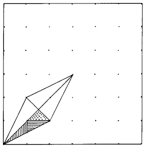
Figure 1: The affine family ${\bf F}(x_{1},x_{2})$ is divided into 144 equivalent triangles of equal area, as described in the text. The lattice shown in the background are the 6th roots.

There are equivalence relations connecting different matrices within this family. They form a discrete group, and thus they will affect the size but not the dimensionality of the affine family. Let us think of the parameter space as a square in the $(x_{1},x_{2})$ plane (see fig. 1). By inspection one finds cyclic translation groups of order 6:

$${\bf F}(x_{1},x_{2})\approx{\bf F}(x_{1}+2/6,x_{2}+1/6)\approx{\bf F}(x_{1}+4/6,x_{2}+2/6)\approx{\bf F}(x_{1},-x_{2}),$$

(5)

$${\bf F}(x_{1},x_{2})\approx{\bf F}(x_{1}+1/6,x_{2}+2/6)\approx{\bf F}(x_{1}+2/6,x_{2}+4/6)\approx{\bf F}(-x_{1},x_{2}).$$

They divide the square into $12$ copies of a fundamental region that is a parallellogram. There are further equivalences corresponding to transformations of order $2$. By inspection

$${\bf F}(x_{1},x_{2})\approx{\bf F}(x_{2},x_{1})\ .$$ (6)

If we permute the rows and then dephase the row that ends up in the first place, we find that

$${\bf F}(x_{1},x_{2})\approx{\bf F}(-x_{1},-x_{2})\ .$$ (7)

As a result, our parallellogram will be divided into four equivalent triangles. Finally we can permute the columns and dephase the column that ends up in the first place. This gives a final cyclic equivalence group of order 3:

$${\bf F}(x_{1},x_{2})\approx{\bf F}(x_{2}-x_{1},-x_{1})\approx{\bf F}(-x_{2},x_{1}-x_{2})$$ (8)

Considered as transformations of our square, these last transformations are not isometries but they do preserve area. Hence the triangles that we had in the previous step are themselves divided into three triangles of equal area, one of which is our final fundamental region of inequivalent Hadamard matrices. A convenient choice of fundamental region is a triangle with corners at $(0,0)$, $(1/6,0)$ and $(1/6,1/12)$; the original square is covered by $144$ copies of this region. The family ${\bf F}^{\rm T}(x_{1},x_{2})$ works (at this stage) in an entirely analogous way.

Björck’s circulant Hadamard matrix is

$${\bf C}=\left[\begin{array}[]{cccccc}1&id&-d&-i&-\bar{d}&i\bar{d}\\ i\bar{d}&1&id&-d&-i&-\bar{d}\\ -\bar{d}&i\bar{d}&1&id&-d&-i\\ -i&-\bar{d}&i\bar{d}&1&id&-d\\ -d&-i&-\bar{d}&i\bar{d}&1&id\\ id&-d&-i&-\bar{d}&i\bar{d}&1\end{array}\right]\ ,\hskip 17.07164pt\bar{d}d=1\ .$$ (9)

See section 6 for further discussion of circulant Hadamard matrices. The complex number $d$ has modulus unity and is

$$d=\frac{1-\sqrt{3}}{2}+i\sqrt{\frac{\sqrt{3}}{2}}\hskip 14.22636pt\Rightarrow\hskip 14.22636ptd^{2}-(1-\sqrt{3})d+1=0\ .$$ (10)

No affine family stems from this matrix [11]. We will have more to say about this matrix later; for now let us just mention that all Hadamard matrices equivalent to a circulant matrix have been listed by Björck and coauthors [16], for $N\leq 8$.

The Diţă family is

$${\bf D}(x)=\frac{1}{\sqrt{6}}\left[\begin{array}[]{cccccc}1&1&1&1&1&1\\ 1&-1&i&-i&-i&i\\ 1&i&-1&iz&-iz&-i\\ 1&-i&i\bar{z}&-1&i&-i\bar{z}\\ 1&-i&-i\bar{z}&i&-1&i\bar{z}\\ 1&i&-i&-iz&iz&-1\end{array}\right]\ ,\hskip 17.07164ptz\equiv e^{2\pi ix}\ .$$ (11)

There are equivalence relations within this family too. In fact

$${\bf D}(x)\approx{\bf D}(x+1/2)\approx{\bf D}(-x+1/4)\ .$$ (12)

Hence we can take $-1/8\leq x\leq 1/8$ without loss of generality. The matrices ${\bf D}(x)$ can be written on block circulant form; see section 7.

The Hermitian family ${\bf B}(\theta)$ was found very recently, by Beauchamp and Nicoara [17], and consists—up to equivalences—of all Hermitian Hadamard matrices of order 6. Explicitly it is

$${\bf B}(\theta)=\frac{1}{\sqrt{6}}\left[\begin{array}[]{cccccc}1&1&1&1&1&1\\ 1&-1&-\bar{x}&-y&y&\bar{x}\\ 1&-x&1&y&\bar{z}&-\bar{t}\\ 1&-\bar{y}&\bar{y}&-1&-\bar{t}&\bar{t}\\ 1&\bar{y}&z&-t&1&-\bar{x}\\ 1&x&-t&t&-x&-1\end{array}\right]$$ (13)

where $(x,y,z,t)$ are complex numbers of modulus one, related by

$$y=e^{i\theta}\hskip 56.9055ptt=xyz$$ (14)

$$z=\frac{1+2y-y^{2}}{y(-1+2y+y^{2})}$$ (15)

$$x=\frac{1+2y+y^{2}\pm\sqrt{2}\sqrt{1+2y+2y^{3}+y^{4}}}{1+2y-y^{2}}\ ,$$ (16)

with $\theta$ providing a free parameter. The two branches of the square root lead to equivalent families. This is an example of a non-affine family (and the only such example known to us for $N=6$).

The phase $\theta$ cannot be chosen arbitrarily; an interval around $\theta=0$ is excluded. The Hadamard property requires that

$$|y|^{2}=1\hskip 14.22636pt\Rightarrow\hskip 14.22636pt|x|^{2}=|z|^{2}=|t|^{2}=1\ .$$ (17)

On examining this point one sees that this restricts the allowed values of $y=\cos{\theta}+i\sin{\theta}$. There are no difficulties with $z$, but the numerator of $x$ becomes

$$1+2y+y^{2}\pm\sqrt{2}\sqrt{1+2y+2y^{3}+y^{4}}=2y(1+\cos{\theta}\pm\sqrt{2\cos{\theta}+2\cos^{2}{\theta}-1}).$$ (18)

The absolute value of this expression hinges crucially on the sign inside the square root; the absolute value of $x$ will be equal to one if that sign is negative. This restricts the phase to

$$\cos{\theta}\leq\frac{\sqrt{3}-1}{2}\ .$$ (19)

The allowed range of $\theta$ has end points, with vanishing square root, at $y=-\bar{d}$ and $y=-d$. The curve is not closed; its end points correspond to permutations of Björck’s matrix ${\bf C}$ and its complex conjugate. This is also the case if $y=\bar{d}^{2}$ or $y=d^{2}$. If $y=-1$ or $y=\pm i$ we obtain permutations of Diţă’s matrix.

Tao’s matrix never appeared in our searches for MUBs, so we do not give it explicitly here. Since Tao’s matrix is composed of 3d roots only, one may ask whether there are any $N=6$ Hadamard matrices based only on 5th or 7th roots. Using a computer program to be described in section 5 we have shown that no such Hadamard matrix exists.

3. Preliminaries on MUBs

We now turn to Mutually Unbiased Bases, or MUBs. First we recall some definitions. Fix an orthonormal basis $|e_{a}\rangle$ in an $N$ dimensional Hilbert space. A unit vector $|f\rangle$ is said to be unbiased with respect to the fixed basis if for all $a$

$$|\langle e_{a}|f\rangle|^{2}=\frac{1}{N}\ .$$ (20)

The important thing is that the right hand side is constant; its value is a consequence. A pair of orthonormal bases is said to be an unbiased pair if all the vectors in one of the bases are unbiased with respect to the other. One can go on to define larger sets of mutually unbiased bases, or MUBs, in the obvious way. It is known that the number of MUBs one can find is bounded from above by $N+1$, but it is not known if this bound can be achieved unless $N$ is a power of a prime number. A set of $N+1$ MUBs, if it exists, is known as a complete set.

If one member of a set of MUBs is represented by the columns of the unit matrix, all the other bases must be represented by the columns of a set of Hadamard matrices. A complete set of $N+1$ MUBs exists if we can find $N$ enphased Hadamard matrices representing bases that are MUB with respect to each other. Altogether then we have $N$ Hadamard matrices that are said to be Mutually Unbiased Hadamards, or MUHs [11]. Note that two Hadamard matrices $H_{1},H_{2}$ are unbiased if and only if

$$H^{\dagger}_{1}H_{2}=H_{3}\ ,$$ (21)

where $H_{3}$ is an Hadamard matrix too. We say that a set of MUHs all of whose members are equivalent in the sense of section 2 is homogeneous, otherwise it is heterogeneous. The standard construction of complete sets of MUBs in prime power dimensions [4] gives a homogeneous set of $N$ MUHs.

When are two pairs of MUBs equivalent to each other? Let $(M_{0},M_{1})$ denote an ordered pair of MUBs, and $\{M_{0},M_{1}\}$ an unordered pair, with each basis represented as the columns of a unitary matrix. We are not interested in the order of the constituent vectors, nor in the phase factors multiplying these vectors. Hence, with $P$ a permutation and $D$ a diagonal unitary matrix,

$$(M_{0}PD,M_{1}P^{\prime}D^{\prime})\approx(M_{0},M_{1})\ .$$ (22)

We also declare that an overall unitary transformation of the Hilbert space is irrelevant, so that

$$(UM_{0},UM_{1})\approx(M_{0},M_{1})\ .$$ (23)

Then the pair can always be represented in the form $({{\hbox{{\rm 1}\kern-2.59995pt\hbox{\rm l}}}},H)$, where $H$ is an Hadamard matrix. It follows that the equivalence relation (3), used for Hadamard matrices, is the correct equivalence relation also for ordered MUB pairs;

$$({{\hbox{{\rm 1}\kern-2.59995pt\hbox{\rm l}}}},H_{1})\approx({{\hbox{{\rm 1}\kern-2.59995pt\hbox{\rm l}}}},H_{2})\hskip 14.22636pt\Leftrightarrow\hskip 14.22636ptH_{1}\approx H_{2}\ .$$ (24)

From eq. (23) we know that $({{\hbox{{\rm 1}\kern-2.59995pt\hbox{\rm l}}}},H)\approx(H^{\dagger},{{\hbox{{\rm 1}\kern-2.59995pt\hbox{\rm l}}}})$. For unordered MUB pairs this means that

$$\{{{\hbox{{\rm 1}\kern-2.59995pt\hbox{\rm l}}}},H\}\approx\{{{\hbox{{\rm 1}\kern-2.59995pt\hbox{\rm l}}}},H^{\dagger}\}\ .$$ (25)

Therefore, the condition for unordered pairs to be equivalent is

$$\{{{\hbox{{\rm 1}\kern-2.59995pt\hbox{\rm l}}}},H_{1}\}\approx\{{{\hbox{{\rm 1}\kern-2.59995pt\hbox{\rm l}}}},H_{2}\}\hskip 14.22636pt\Leftrightarrow\hskip 14.22636pt\begin{array}[]{ll}\mbox{either}\ H_{1}\approx H_{2}&\\ &\\ \mbox{or}\ H_{1}\approx H_{2}^{\dagger}&\ .\end{array}$$ (26)

The discussion can be extended to larger sets of MUBs, ordered or unordered —although the equivalences will become harder to check as the number of MUBs increases.

For the Hadamard matrices we know, it is true that

$$[{\bf F}(x_{1},x_{2})]^{\dagger}\approx{\bf F}^{\rm T}(x_{1},x_{2})$$ (27)

$$[{\bf D}(x)]^{\dagger}\approx{\bf D}(-x)$$ (28)

$${\bf C}^{\dagger}\approx{\bf C}\hskip 34.1433pt{\bf S}^{\dagger}\approx{\bf S}\ ,$$ (29)

and finally the Beauchamp-Nicoara family is Hermitian by construction. Thus the set of unordered MUB pairs is smaller than the set of inequivalent Hadamard matrices. In particular, $\{{{\hbox{{\rm 1}\kern-2.59995pt\hbox{\rm l}}}},{\bf F}(x_{1},x_{2})\}$ and $\{{{\hbox{{\rm 1}\kern-2.59995pt\hbox{\rm l}}}},{\bf F}^{\rm T}(x_{1},x_{2})\}$ are equivalent when considered as unordered pairs.

Let us return to the MUBs themselves. It is useful to think of them as sets of density matrices, rather than as sets of vectors in Hilbert space. Recall that a unit vector $|e\rangle$ in an $N$ dimensional Hilbert space corresponds to a projector $|e\rangle\langle e|$, which is an Hermitian matrix of trace unity, and as such can be regarded as a vector in an $N^{2}-1$ real dimensional vector space whose elements are matrices. The origin of this vector space is naturally chosen to sit at the matrix $\rho_{*}=\frac{1}{N}{{\hbox{{\rm 1}\kern-2.59995pt\hbox{\rm l}}}}$, and then its vectors are traceless matrices. Explicitly the correspondence is

$$|e\rangle\hskip 14.22636pt\rightarrow\hskip 14.22636pt{\bf e}=\sqrt{\frac{2N}{N-1}}\left(|e\rangle\langle e|-\rho_{\star}\right)\ .$$ (30)

The vector ${\bf e}$ is a unit vector with respect to the scalar product

$${\bf e}\cdot{\bf f}=\frac{1}{2}\mbox{Tr}\ {\bf e}{\bf f}\ .$$ (31)

The distance between two matrices $A$ and $B$ is given by

$$d^{2}(A,B)=\frac{1}{2}\mbox{Tr}(A-B)^{2}\ .$$ (32)

This is the Euclidean Hilbert-Schmidt distance.

It is important to realize that although any unit vector in Hilbert space gives rise to a unit vector in the larger space, it is only a small subset of the latter that can be realized in this way. The convex cover of this small subset is the set of all density matrices (or quantum states). An orthonormal basis in the Hilbert space corresponds to $N$ vectors that form a regular simplex in the larger space. This simplex spans an $N-1$ dimensional plane through the origin. It is moreover easy to see that

$$|\langle e|f\rangle|^{2}=\frac{1}{N}\hskip 14.22636pt\Leftrightarrow\hskip 14.22636pt{\bf e}\cdot{\bf f}=0\ .$$ (33)

Therefore, if the unit vectors belong to a pair of MUBs, the corresponding vectors in the large vector space are orthogonal. It follows that a pair of MUBs span two totally orthogonal $(N-1)$-planes through the origin. This fact is at the bottom of the reason why MUBs are useful in quantum state tomography [4]. And we see immediately that there can be at most $N+1$ MUBs, since there is no room for more than $N+1$ totally orthogonal $(N-1)$-planes in an $N^{2}-1$ dimensional space.

4. Interlude: a distance between bases

We need a distance between bases in Hilbert space, such that it becomes maximal if the bases are MUB. It should be natural and easy to compute, but we do not insist on any precise operational meaning for it.

As explained in section 3, a basis in an $N$ dimensional Hilbert space spans an $(N-1)$-plane in a real vector space of $N^{2}-1$ dimensions. There is a standard way to define a distance between such planes, namely to regard them as points in a Grassmannian, in itself embedded in the surface of a sphere within an Euclidean space of a quite high dimension [21]. The procedure is analogous to the one we followed when we transformed our Hilbert space vectors into points in a space embedded within the space of traceless matrices. The details are as follows. Starting from a basis $|e_{a}\rangle$ in Hilbert space, use the recipe given in eq. (30) to form the $N$ vectors ${\bf e}_{a}$. Expand these vectors relative to a basis. Then form the $(N^{2}-1)\times N$ matrix

$$B=\sqrt{\frac{N-1}{N}}[{\bf e}_{1}\ {\bf e}_{2}\ \dots\ {\bf e}_{N}]\ .$$ (34)

It has rank $N-1$. Next introduce an $(N^{2}-1)\times(N^{2}-1)$ matrix of trace $N-1$, projecting onto the $(N-1)$ dimensional plane spanned by the ${\bf e}_{a}$:

$$P=B\ B^{\rm T}=\frac{N-1}{N}[{\bf e}_{1}\ \dots\ {\bf e}_{N}]\left[\begin{array}[]{c}{\bf e}^{\rm T}_{1}\\ \dots\\ {\bf e}_{N}^{\rm T}\end{array}\right]\ .$$ (35)

It is easy to check (through acting on ${\bf e}_{a}$ say) that this really is a projector. The chordal Grassmannian distance between two $(N-1)$-planes is defined in terms of the corresponding projectors as

$$D^{2}_{c}(P_{1},P_{2})=\frac{1}{2(N-1)}\mbox{Tr}(P_{1}-P_{2})^{2}=1-\frac{1}{N-1}\mbox{Tr}P_{1}P_{2}\ .$$ (36)

There is an analogy to how the density matrices were defined in the first place, and to the Hilbert-Schmidt distance between them.

We can think of the projectors $P$ as points on the surface of a sphere in ${\bf R}^{M}$, where—as it happens—

$$M=\frac{N^{4}-N^{2}-2}{2}\ .$$ (37)

This explains the name “chordal distance”. It is however important to realize that the Grassmannian of $(N-1)$-planes forms a very small subset of this sphere. Its dimension is $N(N-1)^{2}$. And then bases in Hilbert space correspond to a small subset of the Grassmannian.

The chordal distance has been used in studies of packing problems for planes and subspaces [22]. It has a number of advantages when compared to more sophisticated distances, such as the geodesic distance within the Grassmannian (which would be analogous to the Fubini-Study distance between pure quantum states). It is useful to know that the chordal distance can be written as a function of the principal angles $\theta_{i}$, namely

$$D^{2}_{c}=1-\frac{1}{N-1}\sum_{i=1}^{N-1}\cos^{2}{\theta_{i}}=\frac{1}{N-1}\sum_{i=1}^{N-1}\sin^{2}{\theta_{i}}\ .$$ (38)

Here the first principal angle is defined as

$$\cos{\theta_{1}}=\max{\bf u}_{1}\cdot{\bf v}_{1}\ ,$$ (39)

where ${\bf u}_{1}$ and ${\bf v}_{1}$ are unit vectors belonging to the respective $(N-1)$-planes, chosen so that their scalar product is maximized. The second principal angle is defined by maximizing the scalar product between unit vectors in the orthogonal complements to ${\bf u}_{1}$ and ${\bf v}_{1}$, and so on. It is then clear that

$$0\leq D^{2}_{c}\leq 1-\frac{k}{N-1}\ ,$$ (40)

where $k$ is the dimension of the intersection of the two planes. The distance is maximal if and only if the $(N-1)$-planes are totally orthogonal.

Now consider two $(N-1)$-planes spanned by vectors corresponding to two bases $|e_{a}\rangle$ and $|f_{a}\rangle$ in Hilbert space. Working through the details, one finds that the distance squared between the bases is

$$D_{c}^{2}(P_{1},P_{2})=1-\frac{1}{N-1}\sum_{a=0}^{N-1}\sum_{b=0}^{N-1}\left(|\langle e_{a}|f_{b}\rangle|^{2}-\frac{1}{N}\right)^{2}\ .$$ (41)

Thus, between bases in Hilbert space,

$$0\leq D^{2}_{c}\leq D_{\rm max}^{2}=1\ .$$ (42)

The distance attains its maximum value if and only if the bases are MUB. A set of MUBs forms a regular equatorial simplex on the sphere in ${\bf R}^{M}$, although there will be many regular equatorial simplices that do not arise in this way.

What is $D^{2}_{c}$ on the average, for two bases picked at random in Hilbert space? To answer this question we represent one basis by the standard basis. Then we choose a vector at random according to the Fubini-Study measure, choose a vector in its orthogonal complement again according to the Fubini-Study measure (in one dimension lower), and so on until we have a complete basis. The resulting measure is a measure on the flag manifold $U(N)/[U(1)]^{N}$. In practice the calculation is simple; the average is

$$\left<D^{2}_{c}\right>=\left<1-\frac{1}{N-1}\sum_{a}\sum_{b}\left(|\langle e_{a}|f_{b}\rangle|^{2}-\frac{1}{N}\right)^{2}\right>\ .$$ (43)

Using the linearity of the average, together with the fact that the $N^{2}$ terms in the sum must have equal averages, we can rewrite this as

$$\left<D^{2}_{c}\right>=1-\frac{N^{2}}{N-1}\left<\left(|\langle e_{0}|f_{0}\rangle|^{2}-\frac{1}{N}\right)^{2}\right>\ ,$$ (44)

Hence it is enough to calculate the average of a function of the modulus of a component of a random vector, using the Fubini-Study measure. How to do this is described elsewhere [23, 21]; the answer we arrive at is

$$\left<D^{2}_{c}\right>=\frac{N}{N+1}\ .$$ (45)

For $N=6$ we have $\left<D^{2}_{c}\right>=0.86$; as $N$ grows the average distance squared approaches the maximum value $1$. Note that the average depends smoothly on $N$, whatever the maximal number of MUBs in $N$ dimensions may be.

One can ask for a function of $N+1$ points on the sphere in ${\bf R}^{M}$, whose maximum is attained when the points form a regular equatorial simplex. Given that $N+1\leq M$ it happens that

$$f=\sum_{i=1}^{N+1}\sum_{j=1}^{N+1}D^{2}_{c}(P_{i},P_{j})\ ,$$ (46)

is such a function. To see this, use the Euclidean norm on the space in which the Grassmannian of $(N-1)$-planes is embedded, and normalise it so that the projectors correspond to $N+1$ unit vectors ${\bf E}_{i}$. Then

$$\sum_{i<j}||{\bf E}_{i}-{\bf E}_{j}||^{2}=N(N+1)-2\sum_{i<j}{\bf E}_{i}\cdot{\bf E}_{j}\ .$$ (47)

On the other hand

$$N+1+2\sum_{i<j}{\bf E}_{i}\cdot{\bf E}_{j}=||\sum_{i}{\bf E}_{i}||^{2}\geq 0\ .$$ (48)

A minimum of the last expression corresponds to a maximum of the function $f$. A regular equatorial simplex clearly saturates the inquality (48), given that $N+1$ is smaller than the dimension of the space that we are in. This proves our point. There are other configurations besides the desired one that also saturate the bound. Since they do not arise from bases in the underlying Hilbert space we can ignore such configurations. Still we do not claim that $f$ is the most useful function of its kind.

Equipped with our notion of distance (so that we can quantify our failures), we can look for complete sets of 7 MUBs in ${\bf C}^{6}$. The natural way to proceed, given the results of this section, is to maximise the function

$$f=\sum_{i=1}^{7}\sum_{j=1}^{7}D^{2}_{c}(P_{i},P_{j})=\sum_{i=1}^{7}\sum_{j=1}^{7}\left(1-\frac{1}{5}\sum_{a=0}^{5}\sum_{b=0}^{5}\left(|\langle e^{(i)}_{a}|e^{(j)}_{b}\rangle|^{2}-\frac{1}{N}\right)^{2}\right)\ ,$$ (49)

with the understanding that the $|e^{(i)}_{a}\rangle$ are orthonormal bases in Hilbert space. There is no a priori reason to believe that the upper bound on $f$ can be attained, because we are confined to a small subset of all possible $(N-1)$-planes. Still, it might be interesting to find the “best” solution in this sense. A similar but more sophisticated procedure has been successfully used to find a special kind of overcomplete bases known as SIC-POVMs [24]. We have not attempted such a calculation however.

5. MUBs composed from rational roots of unity

In our search for MUBs we rely on the classification of ordered MUB pairs through Hadamard matrices. Without loss of generality we assume that the first MUB is represented by the standard basis 1l, and call it $(\mbox{MUB})_{0}$. Then we choose a representative of an equivalence class of Hadamard matrices, and call it $(\mbox{MUB})_{1}$. Assume it to be given in dephased form. All bases that are MUB with respect to the first two must then be represented by enphased Hadamard matrices, and we proceed to look for them.

For $N\leq 5$ there exist maximal sets of $N+1$ MUBs, and these sets are unique up to an overall unitary transformation. Given that $(\mbox{MUB})_{1}$ is not unique for $N=4$, this is perhaps a little surprising. But for $N=4$ it is possible to find inequivalent and incomplete sets of MUBs, that cannot be extended to complete sets [25]. To get the complete set one must start with the real Hadamard matrix, rather than the Fourier matrix, as $(\mbox{MUB})_{1}$. Given that Hadamard matrices of order 6 are highly non-unique, the question where to place $(\mbox{MUB})_{1}$ becomes non-trivial for $N=6$.

All known complete sets of MUBs are built from vectors all of whose components are $N$th or $2N$th roots of unity, depending on whether the dimension $N$ is odd or even [4, 26]. We therefore made a program that lists, for $N=6$, all orthonormal bases whose vectors are composed of 12th roots. They are candidates for $(\mbox{MUB})_{1}$. Next, for each $(\mbox{MUB})_{1}$ the program lists the set of all vectors composed from 12th roots and unbiased with respect to it. The program also lists all orthonormal bases that can be constructed from each set of unbiased vectors. They are candidates for $(\mbox{MUB})_{2}$. Finally we prune the list so that it contains only inequivalent Hadamard matrices as $(\mbox{MUB})_{1}$, and if there are several $(\mbox{MUB})_{2}$ we compute the distance between them to see if we get any sets of four MUBs in this way. Note that this means that the part of the landscape of Hadamard matrices we search in consists of the Fourier and Diţă families, the Tao matrix, enphased versions of these, and (probably) nothing more. The analogous calculation when $N$ is a power of a prime would have found all known complete sets of MUBs, but for $N=6$ only triplets of MUBs turned up.

The 12th roots list we arrived at is

${\bf F}(0,0)$ admits 4 candidates for $(\mbox{MUB})_{2}$.

${\bf F}(1/6,0)$ admits 1 candidate for $(\mbox{MUB})_{2}$.

${\bf F}^{\rm T}(1/6,0)$ admits 1 candidate for $(\mbox{MUB})_{2}$.

This is all. The 4 bases that are MUB with respect to ${\bf F}(0,0)$ will be discussed in the next section, the basis that is MUB with respect to ${\bf F}^{\rm T}(1/6,0)$ is an enphased version of ${\bf F}(0,0)$, while the basis that is MUB with respect to ${\bf F}(1/6,0)$ is an enphased version of itself.

We redid the entire calculation using 24th roots. This resulted in the following additional entries in the list:

${\bf F}(1/6,1/12)$ admits 4 candidates for $(\mbox{MUB})_{2}$.

${\bf D}(1/8)$ admits 4 candidates for $(\mbox{MUB})_{2}$.

Again this is all; these results are illustrated in fig. 2. In the picture the asymmetry between ${\bf F}(x_{1},x_{2})$ and ${\bf F}^{\rm T}(x_{1},x_{2})$ looks quite odd. From section 3, and from eq. (27) in particular, we know that the unordered MUB pairs $\{{{\hbox{{\rm 1}\kern-2.59995pt\hbox{\rm l}}}},{\bf F}(1/6,1/12)\}$ and $\{{{\hbox{{\rm 1}\kern-2.59995pt\hbox{\rm l}}}},{\bf F}^{\rm T}(1/6,1/12)\}$ are equivalent, so they should have the same number of $(\mbox{MUB})_{2}$ candidates. In section 7 it will be seen that, in fact, they do—although in one case none of the candidates is built from 24th roots only.

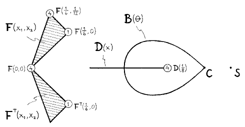
Figure 2: Here we show all MUB pairs that can be extended to triplets of MUBs, and how many triplets there are for each such pair, under the restriction that only 24th roots are used. The background for the picture is the set of all known equivalence classes of $N=6$ Hadamard matrices.

We redid the calculation using 48th, 72th, and 60th roots; $48=2^{4}\cdot 3$ and $72=2^{3}\cdot 3^{2}$ seemed like reasonable things to try, while $60=2^{2}\cdot 3\cdot 5$ was a wild shot. Anyway the list did not increase. It is tempting to think of vectors composed of 24th roots as forming a grid in a relevant part of Hilbert space. Through a study of the distances between the candidate $(\mbox{MUB})_{2}$ we could have refined the grid in interesting places, but we did not pursue this—the grid is not very dense.

6. MUB triplets including the Fourier matrix

Let us consider the case when $(\mbox{MUB})_{1}$ is the Fourier matrix. Here we do not have to rely on our own calculations, because complete results are available: using the symbolic manipulation program MAGMA, Grassl [14] has computed all vectors unbiased with respect to both the standard and the Fourier basis. The same calculation was in fact done earlier by Björck and coworkers [15, 16]. There are 48 such vectors altogether, or 24 vectors and their complex conjugates. Each vector shows up in two different bases, so they form 16 bases altogether. Using the classification of Hadamard matrices, the 16 $(\mbox{MUB})_{2}$ turn out to form four groups:

(i) Two circulant Fourier matrices enphased with 12th roots of unity; “$\omega{\bf F}$”.
(ii) Two matrices equivalent to ${\bf F}^{\rm T}(1/6,0)$, and enphased with 12th roots of unity; “$\omega{\bf F}^{\rm T}$”.
(iii) Six circulant Björck matrices ${\bf C}$ (three with $d$ and three with $\bar{d}$), enphased with 12th roots of unity; “$\omega{\bf C}$”.
(iv) Six Fourier matrices enphased with products of Björck’s magical number $d$ (and $\bar{d}$) and 12th roots of unity; “$d\omega{\bf F}$”.

See eq. (10) for the definition of $d$. We will refer to the bases in groups (i) and (ii) as classical, and to the remaining bases as non-classical, for a reason that will transpire. The matrices in groups (i) and (iii) are circulant when their columns are multiplied by suitable phase factors. They already include all vectors unbiased with the Fourier matrix. Both the $\omega{\bf F}^{\rm T}$ matrices contain three columns each from the two $\omega{\bf F}$ matrices. Each matrix $d\omega{\bf F}$ contains one vector from each matrix $\omega{\bf C}$, and vice versa. The four groups of bases are invariant under complex conjugation. Two of the bases in $\omega{\bf C}$, namely those given by Björck’s matrix with $d$ and with $\bar{d}$, are unchanged by complex conjugation.

The distances between the 16 bases are as follows: The classical bases form a perfect square, with edge lengths squared $D_{c}^{2}=0.4$ (and the enphased Fouriers in opposite corners). The distance between any classical and any non-classical basis is always given by $D^{2}_{c}=0.92$. The distance between any member of group (iii) to any member of group (iv) is always $D^{2}_{c}=0.74$. Finally the distance relations within the two groups of 6 are identical; each group contains two equilateral triangles with edge lengths $D^{2}_{c}=0.93$. These triangles are exchanged if $d$ and $\bar{d}$ are exchanged. In addition, within each group each basis has two bases at $D^{2}_{c}=0.86$ and one at $D^{2}_{c}=0.88$.

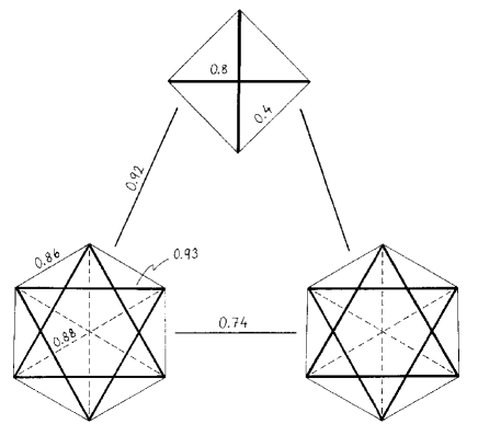
Figure 3: All Hadamard bases MUB with respect to ${\bf F}$ (a single point in fig. 2). The square consists of (enphased, affine) Fouriers, one of the two David’s stars of Björck matrices enphased with 12th roots, and the other of Fouriers enphased with the number $d$. The numbers refer to the chordal distance squared, $D^{2}_{c}$.

The Björck/Grassl results are summarised in fig. 3. There does not exist any set of four MUBs including 1l and ${\bf F}$, since the distance squared between any possible pair of $(\mbox{MUB})_{2}$ never reaches 1. The best we can do with 7 bases is $D^{2}_{c}\geq 0.86$. This can be compared to random searches; in a sample of 20 million bases, chosen according to the measure described in section 4, the best results were $D^{2}_{c}\geq 0.91$ for 4 bases, and $D^{2}_{c}\geq 0.86$ for 7 bases.

It is striking that every vector vector unbiased with respect to 1l and ${\bf F}$ can be collected into some $(\mbox{MUB})_{2}$. The “doubling” of the non-classical bases is striking too. To explain these features we begin by proving that a vector is unbiased with respect to both 1l and ${\bf F}$ if and only if it is a member of a circulant Hadamard matrix. This requires us to recount some well known facts about the discrete Fourier transform. Given a sequence of complex numbers $z_{a}$, $0\leq a\leq N-1$, we define its Fourier transform to be

$$\tilde{z}_{a}=\frac{1}{\sqrt{N}}\sum_{b=0}^{N-1}q^{ab}z_{b}\ .$$ (50)

In condensed notation

$$\tilde{z}={\bf F}z\hskip 14.22636pt\Leftrightarrow\hskip 14.22636ptz={\bf F}^{\dagger}\tilde{z}\ .$$ (51)

If we are given a sequence of complex numbers $z_{a}$, the column vector whose components are $\tilde{z}_{a}/\sqrt{N}$ is unbiased with respect to the Fourier basis if and only if the sequence $z_{a}$ is unimodular, $|z_{a}|^{2}=1$, and it is unbiased with respect to the standard basis if and only if $\tilde{z}_{a}$ is unimodular. Hence vectors that are unbiased with respect to both the standard basis and the Fourier basis are in one-to-one correspondence to sequences obeying

$$|z_{a}|^{2}=|\tilde{z}_{a}|^{2}=1$$ (52)

for all values of $a$. Such sequences are called biunimodular. (Standard conventions for the Fourier transform sit a little uneasily with our conventions for MUBs. We decided to live with this, which is why our vectors are made from $\tilde{z}_{a}$ rather than $z_{a}$ itself.)

Biunimodular sequences have an interesting property, that emerges when one studies the autocorrelation function

$$\gamma_{b}\equiv\frac{1}{N}\sum_{a=0}^{N-1}\bar{\tilde{z}}_{a}\tilde{z}_{a+b}\ .$$ (53)

An easy calculation shows that

$$\gamma_{b}=\frac{1}{N}\sum_{a=0}^{N-1}|z_{a}|^{2}q^{ab}\ .$$ (54)

Hence, if the sequence is biunimodular it obeys

$$\gamma_{b}=\delta_{b,0}\ .$$ (55)

Therefore $\tilde{z}_{a}$ and $\tilde{z}_{a+b}$, with $b$ fixed and non-zero, are orthogonal vectors.

A matrix is called circulant if it takes the form

$$C=\left[\begin{array}[]{cccc}\tilde{z}_{0}&\tilde{z}_{N-1}&\dots&\tilde{z}_{1}\\ \tilde{z}_{1}&\tilde{z}_{0}&\dots&\tilde{z}_{2}\\ \vdots&\vdots&&\vdots\\ \tilde{z}_{N-1}&\tilde{z}_{N-2}&\dots&\tilde{z}_{0}\end{array}\right]\ .$$ (56)

The matrix elements are

$$C_{ab}=\tilde{z}_{a-b}\ .$$ (57)

With this definition a circulant matrix is Hadamard (up to normalisation) if and only if the sequence $z_{a}$ is biunimodular. It follows that all vectors unbiased with respect to both the standard and the Fourier bases can be collected into a set of circulant Hadamard matrices whose columns form bases that are MUB with respect to the standard and Fourier bases.

This explains why all the 48 unbiased vectors are included in some basis that can be represented by an Hadamard matrix in circulant form. It remains to understand the “doubling” of bases found in Grassl’s list. For any circulant matrix $C$, with first column $\tilde{z}_{a}$, it is easy to check that

$${\bf F}^{\dagger}C=D{\bf F}^{\dagger}\ ,\hskip 22.76219ptD=\mbox{diag}(z_{0},z_{1},\dots,z_{N-1})\ .$$ (58)

Together with the earlier results, this entitles us to say that a vector is unbiased with respect to both the standard and the Fourier bases if and only if it is a column of a circulant Hadamard matrix, and every such matrix represents a basis that is MUB with respect to both 1l and ${\bf F}$. Incidentally it also implies that the Fourier matrix diagonalises every circulant matrix. Now consider an unordered MUB triplet $\{{{\hbox{{\rm 1}\kern-2.59995pt\hbox{\rm l}}}},{\bf F},H\}$. From section 3 we know that

$$\{{{\hbox{{\rm 1}\kern-2.59995pt\hbox{\rm l}}}},{\bf F},H\}\approx\{{\bf F}^{\dagger},{{\hbox{{\rm 1}\kern-2.59995pt\hbox{\rm l}}}},{\bf F}^{\dagger}H\}\approx\{{\bf F},{{\hbox{{\rm 1}\kern-2.59995pt\hbox{\rm l}}}},{\bf F}^{\dagger}H\}\ .$$ (59)

In the last step we multiplied ${\bf F}^{\dagger}$ from the right with $P\equiv{\bf F}^{2}$, which is a permutation matrix. Now let $H=C$, a circulant matrix. Using eq. (58)

$$\{{{\hbox{{\rm 1}\kern-2.59995pt\hbox{\rm l}}}},{\bf F},C\}\approx\{{\bf F},{{\hbox{{\rm 1}\kern-2.59995pt\hbox{\rm l}}}},{\bf F}^{\dagger}C\}\approx\{{\bf F},{{\hbox{{\rm 1}\kern-2.59995pt\hbox{\rm l}}}},D{\bf F}^{\dagger}\}\ .$$ (60)

This is how the second “David’s star” of phased Fouriers, in fig. 3, arises. The transformation taking one David’s star to another also exchanges the two enphased Fourier MUBs, while it leaves the pair in group (ii) invariant.

For any dimension the conclusions are, first, that every vector unbiased with respect to both 1l and ${\bf F}$ is given by a biunimodular sequence, and conversely. Second, such a vector exists if and only if it is a member of a circulant basis that forms a MUB triplet with 1l and ${\bf F}$. Third, if this circulant basis is inequivalent (as an Hadamard matrix) to the Fourier matrix then there exists an equivalent MUB triplet whose third member is an enphased Fourier. We have no explanation for the two MUB triplets involving members of the ${\bf F}^{\rm T}$ family—from our point of view they arise by accident.

Counting the number of unbiased vectors, or equivalently biunimodular sequences, remains a dimension dependent matter. By means of symbolic manipulation programs all biunimodular sequences with $N\leq 8$ entries have been listed by Björck and coworkers [15, 16] (see also Haagerup [9]). For $N=6$ there are 48 biunimodular sequences (up to multiplication with a complex phase), or equivalently 48 vectors that are MUB with respect to both the standard and the Fourier bases. This includes 12 classical ones built from 12th roots—they were known to Gauss—and 36 non-classical ones built from Björck’s magical number $d$.

7. MUB triplets with a block structure

In section 5 we observed that there were several MUB triplets built from 24th roots. The ones that cannot be reduced to 12th roots are as follows:

• Starting from the MUB pair $({{\hbox{{\rm 1}\kern-2.59995pt\hbox{\rm l}}}},{\bf D}(1/8))$ we have 4 triplets including enphased versions of ${\bf F}(1/6,1/12)$. They form a semi-regular simplex where 4 edges have $D^{2}_{c}=0.89$ and 2 edges have $D^{2}_{c}=0.95$.

• Starting from the MUB pair $({{\hbox{{\rm 1}\kern-2.59995pt\hbox{\rm l}}}},{\bf F}(1/6,1/12))$ we have 4 triplets including enphased versions of ${\bf D}(1/8)$. They form a regular simplex where all the edges have $D^{2}_{c}=0.93$.

The value $D^{2}_{c}=0.95$ is the largest we have found in our searches for approximate MUB quartets.

These MUB triplets have an interesting structure in common. The affine family including the Fourier matrix, given in eq. (4), consists of Hadamard matrices that are equivalent under permutations to

$${\bf F}(x_{1},x_{2})\approx{\bf F}_{D}\equiv\sqrt{\frac{3}{6}}\left[\begin{array}[]{cc}{\bf F}_{3}&{\bf F}_{3}\\ {\bf F}_{3}D&-{\bf F}_{3}D\end{array}\right]\ ,\hskip 34.1433ptD=\mbox{diag}(1,z_{1},z_{2})\ .$$ (61)

Here ${\bf F}_{3}$ is the 3 by 3 Fourier matrix. This is a kind of twisted version [9, 10] of the tensor product matrix ${\bf F}_{2}\otimes{\bf F}_{3}$.The Diţă family of matrices also has an interesting block structure. It was noted by Zauner that they can always be written on block circulant form, meaning that they can be brought to a form where the matrix consists of four blocks, each of which is a 3 by 3 circulant matrix [12]. This turns out to be relevant here.

Consider the MUB pair $({{\hbox{{\rm 1}\kern-2.59995pt\hbox{\rm l}}}},{\bf F}(1/6,1/12))$. Write it as

$$\left({{\hbox{{\rm 1}\kern-2.59995pt\hbox{\rm l}}}},{\bf F}_{D}\right)\ ,\hskip 28.45274ptD=\mbox{diag}(1,1,\omega^{6})\ ,\hskip 22.76219pt\omega=e^{2\pi i/24}\ .$$ (62)

According to our list this pair can be extended to four triplets including an Hadamard matrix equivalent to ${\bf D}(1/8)$. With the members of the pair fixed according to the above, the four possible choices for $(\mbox{MUB})_{2}$ are

$$\frac{1}{\sqrt{6}}\left[\begin{array}[]{cc}C_{1}&C_{2}\\ C_{2}^{\dagger}&-C_{1}^{\dagger}\end{array}\right]\ ,\hskip 22.76219pt\frac{1}{\sqrt{6}}\left[\begin{array}[]{cc}C_{2}&C_{1}\\ C_{1}^{\dagger}&-C_{2}^{\dagger}\end{array}\right]\ ,$$ (67)

(68)

$$\hskip 39.83385pt\frac{1}{\sqrt{6}}\left[\begin{array}[]{cc}C_{1}^{\dagger}&C_{2}^{\dagger}\\ C_{2}&-C_{1}\end{array}\right]\ ,\hskip 22.76219pt\frac{1}{\sqrt{6}}\left[\begin{array}[]{cc}C_{2}^{\dagger}&C_{1}^{\dagger}\\ C_{1}&-C_{2}\end{array}\right]\ ,$$ (73)

where the $C_{i}$ are the 3 by 3 circulant matrices

$$C_{1}=\left[\begin{array}[]{ccc}1&\omega^{11}&\omega\\ \omega&1&\omega^{11}\\ \omega^{11}&\omega&0\end{array}\right]\ ,\hskip 22.76219ptC_{2}=\left[\begin{array}[]{ccc}1&\omega^{5}&\omega^{7}\\ \omega^{7}&1&\omega^{5}\\ \omega^{5}&\omega^{7}&1\end{array}\right]\ .$$ (74)

In this sense the block structures of the Fourier and Diţă families are related.

We now come to the following little puzzle. We know that

$$\{{{\hbox{{\rm 1}\kern-2.59995pt\hbox{\rm l}}}},\ {\bf F}(1/6,1/12),\ {\bf D}(1/8)\}\approx\hskip 51.21495pt$$

$$\approx\{[{\bf F}(1/6,1/12)]^{\dagger},\ {{\hbox{{\rm 1}\kern-2.59995pt\hbox{\rm l}}}},\ [{\bf F}(1/6,1/12)]^{\dagger}{\bf D}(1/8)\}\approx$$ (75)

$$\approx\{{{\hbox{{\rm 1}\kern-2.59995pt\hbox{\rm l}}}},\ {\bf F}^{\rm T}(1/6,1/12),\ DP[{\bf F}(1/6,1/12)]^{\dagger}{\bf D}(1/8)\}\ ,\hskip 5.69054pt$$

where $DP$ is the product of a diagonal unitary and a permutation matrix. Why then does ${\bf F}^{\rm T}(1/6,1/12)$ not appear in fig. 2? The answer is that the matrix $[{\bf F}(1/6,1/12)]^{\dagger}{\bf D}(1/8)$ is not built from 24th roots only.

What is needed to resolve the puzzle is the number

$$b_{1}=e^{2\pi ic_{1}}\ ,\hskip 22.76219pt\cos{(2\pi c_{1})}=\sqrt{\frac{2}{3}}\ .$$ (76)

We modified the “24th roots program” to allow also $b_{1}$ and $\bar{b}_{1}$ as entries in the vectors. We found the following new MUB triplets:

• Starting from the MUB pair $({{\hbox{{\rm 1}\kern-2.59995pt\hbox{\rm l}}}},{\bf F}^{\rm T}(1/6,1/12))$ we have 4 triplets including enphased versions of ${\bf F}^{\rm T}(c_{1},0)$.

• Starting from the MUB pair $({{\hbox{{\rm 1}\kern-2.59995pt\hbox{\rm l}}}},{\bf F}^{\rm T}(c_{1},0))$ we have 2 triplets including enphased versions of ${\bf F}^{\rm T}(1/6,1/12)$.

• Starting from the MUB pair ${\bf F}(c_{1},0)$ we have 2 triplets including enphased versions of ${\bf D}(-1/8)$.

The first item in this list contains the “missing” triplets whose existence we already knew about—the asymmetries in fig. 2 were due to the 24th roots restriction only.

We have made computer searches to see if we can find other phase factors increasing the number of MUB triplets. One such number turned up, viz.

$$b_{2}=e^{2\pi ic_{2}}\ ,\hskip 22.76219pt\tan{(2\pi c_{2})}=-2\ .$$ (77)

Again we modified the “24th roots program” to allow also $b_{2}$ and $\bar{b_{2}}$ as entries in the vectors. Then we found the following new MUB triplets:

• Starting from the MUB pair $({{\hbox{{\rm 1}\kern-2.59995pt\hbox{\rm l}}}},{\bf D}(0))$ we have 2 triplets including enphased versions of ${\bf F}(9/24+c_{2},0)$. The distance squared between the latter is $D^{2}_{c}=0.77$.

• Starting from the MUB pair $({{\hbox{{\rm 1}\kern-2.59995pt\hbox{\rm l}}}},{\bf F}(9/24+c_{2},0))$ we have 120 vectors unbiased to both, of which 60 vectors form 10 bases that are enphased versions of ${\bf D}(0)$. They form a polytope where 9 edges end at each corner, 6 with $D^{2}_{c}=0.93$ and 3 with $D^{2}_{c}=0.78$.

So we have 6 bases with $D^{2}_{c}\geq 0.93$.

An explicit example of a MUB triplet including $b_{2}$ is

$$\left({{\hbox{{\rm 1}\kern-2.59995pt\hbox{\rm l}}}},{\bf F}_{D},{\bf D}_{\rm bc}\right)\ .$$ (78)

Here $D=\mbox{diag}(\omega^{9}b_{2},1,1)$, ${\bf F}_{D}$ was defined in eq. (61), and ${\bf D}_{\rm bc}$ is a block circulant matrix equivalent to ${\bf D}(0)$, namely

$${\bf D}_{\rm bc}=\frac{1}{\sqrt{6}}\left[\begin{array}[]{cc}C_{3}&C_{4}\\ C_{4}&-iC_{3}^{\dagger}\end{array}\right]\ ,$$ (79)

where

$$C_{3}=\left[\begin{array}[]{ccc}1&\omega^{6}&\omega^{6}\\ \omega^{6}&1&\omega^{6}\\ \omega^{6}&\omega^{6}&1\end{array}\right]\ ,\hskip 22.76219ptC_{4}=\left[\begin{array}[]{ccc}\omega^{15}&\omega^{3}&\omega^{3}\\ \omega^{3}&\omega^{15}&\omega^{3}\\ \omega^{3}&\omega^{3}&\omega^{15}\end{array}\right]\ .$$ (80)

Thus it appears that many of the MUB triplets in this section can be brought to the (twisted product Fourier)—(block circulant Diţă) form. But we did not check them all, nor do we have any complete results analogous to those available for the $({{\hbox{{\rm 1}\kern-2.59995pt\hbox{\rm l}}}},{\bf F})$ pair.

8. What is the most general Hadamard matrix?

We now take up the story of Hadamard matrices again. In section 2 we gave a list of all known Hadamard matrices of order 6, or equivalently of all ordered MUB pairs up to equivalences. The question is whether this list is complete. To investigate this question one can try a perturbative approach to the unitarity equation: multiply the non-trivial matrix elements of a dephased Hadamard matrix with arbitrary phase factors, and solve the unitarity equation to first order in the phases. The number of free parameters that are left when this has been done is an integer known as the defect of the Hadamard matrix. It provides an upper bound on the dimensionality of any analytic set of Hadamard matrices [11].

The defect for the known Hadamard matrices has been computed. For the Fourier, Björck, and Diţă matrices it equals 4, while it equals 0 for Tao’s matrix. Closer inspection shows that the defect is likely to be constant within each affine family, with possible exceptions at isolated values of the affine parameters [11]. We have also computed the defect for one thousand randomly chosen points along the non-affine family ${\bf B}(\theta)$; it was always equal to 4. These results show that Tao’s matrix is an isolated point in the set of all Hadamard matrices. For the remaining matrices the answer is less clear. It appears that their defect is always equal to 4, but the defect provides us with an upper bound on the dimensionality only. It is not known whether the bound is attained, nor indeed whether additional Hadamard matrices, not connected to any of the above, exist.

Let us be fully explicit about the calculation of the defect for Diţă’s matrix ${\bf D}$. We focus on this particular Hadamard matrix because its special form simplifies the resulting calculations. Starting from the known form of the matrix—see eq. (11), with $z=1$—we multiply all non-trivial matrix elements with arbitrary phases according to

$$D_{ab}\rightarrow D_{ab}e^{ix_{ab}}\ ,\hskip 14.22636pt1\leq a,b\leq 5\ .$$ (81)

The unitarity conditions give 15 complex equations, or 30 real equations; more than enough to determine the 25 parameters $x_{ab}$.

We will try to solve the unitarity equations order by order in the phases. If we expand to first order in the phases we obtain the matrix

$$\frac{1}{\sqrt{6}}\left[\begin{array}[]{cccccc}1&1&1&1&1&1\\ 1&-1-ix_{11}&i-x_{12}&-i+x_{13}&-i+x_{14}&i-x_{15}\\ 1&i-x_{21}&-1-ix_{22}&i-x_{23}&-i+x_{24}&-i+x_{25}\\ 1&-i+x_{31}&i-x_{32}&-1-ix_{33}&i-x_{34}&-i+x_{35}\\ 1&-i+x_{41}&-i+x_{42}&i-x_{43}&-1-ix_{44}&i-x_{45}\\ 1&i-x_{51}&-i+x_{52}&-i+x_{53}&i-x_{54}&-1\end{array}\right]\ .$$ (82)

Let us introduce the (unusual) notation $x_{aa}$, $x_{(ab)}$, $x_{[ab]}$ for the diagonal, symmetric off-diagonal, and anti-symmetric parts of $x_{ab}$. One finds that the 30 equations split naturally into

5 equations for $x_{aa}$

10 equations for $x_{(ab)}$

15 equations that split into 6 for $x_{[ab]}$ and 9 for $x_{(ab)}$.

To first order all the equations are linear. There will be 4 undetermined parameters in $x_{[ab]}$. One also finds

$$x_{aa}=0\hskip 34.1433ptx_{(ab)}=0\ .$$ (83)

Since the 19 equations for $x_{(ab)}$ are linear there are no consistency problems. It is however worth observing that the general solution of the final 9 equations for $x_{(ab)}$ is

$$x_{(ab)}=x\ ,$$ (84)

with $x$ remaining as a free parameter, to be set to zero by the other 10 equations for $x_{(ab)}$.

A suitable choice for the free parameters in $x_{[ab]}$ is $x_{[12]}$, $x_{[13]}$, $x_{[24]}$, $x_{[34]}$. Then one finds

$$\begin{array}[]{l}x_{[14]}=x_{[12]}+x_{[34]}\\ x_{[15]}=x_{[13]}+x_{[34]}\\ x_{[23]}=x_{[13]}+x_{[24]}\\ x_{[25]}=-x_{[12]}+x_{[13]}\\ x_{[35]}=-x_{[24]}+x_{[34]}\\ x_{[45]}=-x_{[12]}-x_{[24]}\ .\end{array}$$ (85)

In conclusion, to first order there are 4 free phases, or equivalently the defect equals 4.

We have carried the calculation to third order. However, the Ansatz in eq. (81) must then be modified. Set

$$D_{ab}\rightarrow D_{ab}e^{i(x_{ab}+y_{ab}+z_{ab}+\dots)}=\hskip 165.02597pt$$

(86)

$$=D_{ab}\left(1-\frac{1}{2}x_{ab}^{2}-x_{ab}y_{ab}+i(x_{ab}+y_{ab}+z_{ab}-\frac{1}{6}x_{ab}^{3})+\dots\right)\ .$$

Here it is understood that $y_{ab}$ and $z_{ab}$ are quadratic and cubic functions of $x_{ab}$, respectively. For obvious reasons we do not write out the resulting matrix here. There is an amount of ambiguity in the definition of the higher order terms. This we resolve by imposing

$$y_{[12]}=y_{[13]}=y_{[24]}=y_{[34]}=0\ ,$$ (87)

and analogously at all higher orders. This can always be achieved through a redefinition of the free parameters in $x_{ab}$. Once this is done the expansion in the exponent of eq. (86) is unambiguous.

At each order higher than the first, there will be 30 linear inhomogeneous equations for the $25-4$ new parameters that we introduce, with the inhomogeneous terms made up from products of known lower order contributions. Given eq. (87), the anti-symmetric and diagonal parts will be completely determined. There remain 10 + 9 equations for the symmetric off-diagonal part, and it is not a priori clear that a solution exists.

At second order one finds

$$y_{[ab]}=0$$ (88)

$$\begin{array}[]{l}2y_{11}=-x_{21}^{2}+x_{31}^{2}+x_{41}^{2}-x_{51}^{2}\\ 2y_{22}=-x_{12}^{2}-x_{32}^{2}+x_{42}^{2}+x_{52}^{2}\\ 2y_{33}=x_{13}^{2}-x_{23}^{2}-x_{43}^{2}+x_{53}^{2}\\ 2y_{44}=x_{14}^{2}+x_{24}^{2}-x_{34}^{2}-x_{54}^{2}\\ 2y_{55}=-x_{15}^{2}+x_{25}^{2}+x_{35}^{2}-x_{45}^{2}\ .\end{array}$$ (89)

The last 9 equations imply

$$y_{(ab)}=y\ ,$$ (90)

for some $y$. Detailed examination shows that the remaining 10 equations are consistent with this and with each other. The solution can be written as

$$4y=2y_{11}+2y_{22}-(x_{13}-x_{23})^{2}+(x_{14}-x_{24})^{2}-(x_{15}-x_{25})^{2}\ .$$ (91)

The expansion to second order is therefore consistent.

At third order one finds

$$z_{aa}=0\ ,$$ (92)

together with rather complicated expressions for the part of $z_{[ab]}$ left undetermined by the condition analogous to (87). We do not give them here. The first 10 equations for the symmetric off-diagonal part is solved by

$$z_{(ab)}=0\ .$$ (93)

Thus $z_{ab}$ is, like $x_{ab}$, anti-symmetric in its indices. We are then left with 9 consistency conditions on this solution. Again detailed examination shows that they are obeyed, hence the expansion is consistent to third order.

In conclusion we have proved that Diţă’s matrix admits an expansion to third order in four arbitrary phases. Unfortunately, to second and third order this result depends on cancellations that we do not understand—we have simply checked that they do occur. Nevertheless it seems to us likely that the expansion exists to all orders. This suggests that the parameter space of allowed Hadamard matrices has a four dimensional component.

Some solutions are known to all orders. First of all, if the expression $D_{ab}\rightarrow D_{ab}e^{ix_{ab}}$ is exact, that is if all higher order terms in the exponent vanish, we have an affine family. It is known that Diţă’s matrix admits 5 permutation equivalent affine families [11]. They result from the five choices

$$\begin{array}[]{llll}\mbox{i:}&&(x_{[12]},x_{[13]},x_{[24]},x_{[34]})=(x,0,0,0)&\\ \mbox{ii:}&&(x_{[12]},x_{[13]},x_{[24]},x_{[34]})=(0,x,0,0)&\\ \mbox{iii:}&&(x_{[12]},x_{[13]},x_{[24]},x_{[34]})=(0,0,x,0)&\\ \mbox{iv:}&&(x_{[12]},x_{[13]},x_{[24]},x_{[34]})=(0,0,0,x)&\\ \mbox{v:}&&(x_{[12]},x_{[13]},x_{[24]},x_{[34]})=(x,x,-x,-x)&.\end{array}$$ (94)

In fact our choice of independent variables was made with this result in view. In these cases we have $y_{ab}=z_{ab}=0$, and similarly for all higher order terms, so these solutions are somewhat trivial. Fortunately at least one non-affine family, with non-vanishing higher order terms, is also known to all orders. This is the one-parameter family ${\bf B}(\theta)$, which passes through representatives of the Diţă equivalence class no less than three times. A solution to our equations, equivalent to ${\bf B}(\theta)$ to third order, is

$$(x_{[12]},x_{[13]},x_{[24]},x_{[34]})=(-x,-x,2x,x)\ .$$ (95)

The higher order terms in the exponent of eq. (86) are now non-vanishing. At the same time we observe that, even if it does exist to all orders, this solution must encounter convergence problems in order to reproduce the limits on the phase $\theta$ in the Beauchamp-Nicoara family. Clearly such a problem can occur in the exponent of eq. (86).

Our calculation, together with several different one-parameter solutions known to all orders (one of which is a non-affine solution), does support the conjecture that the set of Hadamard matrices is four dimensional in a neighbourhood of the Diţă matrix. We understand that Beauchamp and Nicoara have numerical evidence for the same state of affairs in a neighbourhood of the Björck matrix [27]. At the same time the existence of Tao’s matrix shows that the set of Hadamard matrices must be disconnected. The Björck and Diţă matrices are connected to each other, but we have no evidence to show how the Fourier matrix fits into the picture.

9. Summary

Mutually unbiased bases live in the landscape of complex Hadamard matrices. A complete classification of the equivalence classes of $N=6$ complex Hadamard matrices, or equivalently of the set of all MUB pairs, is however not available. If we insert arbitrary phases in the known examples, we find that four parameters are left undetermined to first order. The one exception is Tao’s matrix. For Diţă’s matrix we solved the unitarity equations to third order in four arbitrary phases. This does not constitute a proof that the parameter space has a four dimensional component, but we may perhaps quote Lewis Carroll at this point: “I have told you thrice. What I tell you three times is true.”

A set of MUBs can always be described as the standard basis together with a set of Hadamard matrices. We searched for such sets, mostly under the restriction that all vectors be composed from rational roots of unity, but we also gave three examples of non-rational and “MUB-friendly” phase factors. The restriction to rational roots is severe, but the advantage is that systematic searches can be made.

We found only triplets of MUBs. A rich source of triplets is obtained by choosing the Fourier basis as one of the members; the resulting structure can be largely understood through the discrete Fourier transform. Other triplets, with a special block structure, were also found. To add structure to the problem we introduced a natural distance between bases in Hilbert space. It attains its maximum value when the bases are MUB. Whenever a pair of MUBs (including the standard basis) could be extended to a triplet in more than one way, we computed the distance between the possible third members. In this way we found sets of 4 bases where all distances but one are maximal. The highest figure we obtained for the last distance was $D^{2}_{c}=0.95$, significantly closer to the maximum value 1 than is the average distance squared between bases, $\langle D^{2}_{c}\rangle=6/7$.

No-go statements for complete sets of 7 MUBs in $N=6$ have been made. They tend to exclude sets with a high degree of symmetry [13] or with otherwise special group theoretical properties [28], as well as sets constructed using generalisations of methods that work in prime power dimensions [29]. We are unsurprised by our failure to find any complete set—but if our conjecture concerning the set of all Hadamard matrices is true, the no-go theorems are unlikely to apply in general.

So what is the best approximation to a complete set of MUBs that one can find in 6 dimensions? Indeed, what is the maximal number of MUBs one can have in 6 dimensions? The jury is still out.

Note added in proof: After submission of this paper Matolcsi and Szöllosi [30] found a new family of 6  6 Hadamard matrices. And in Ref. [31], Tadej, Życzkowski, and Slomczynski study the defect of unitaries, not necessarily Hadamard.

Acknowledgements:

This work grew out of the Master’s Thesis of one of us (WB). We thank Kyle Beauchamp and Remus Nicoara for sharing their results with us prior to publication, Markus Grassl for sending his vectors for inspection, Bengt Nagel for drawing our attention to the book by Kostrikin and Tiep, and Sören Holst for helping us to the result described in fig. 1.

We acknowledge partial financial support from the Swedish Research Council, from grant PBZ-MIN-008/P03/2003 of the Polish Ministry of Science and Information Technology, and from the European Union research project SCALA.

References

- [1] J. J. Sylvester, Thoughts on inverse orthogonal matrices, simultaneous sign-successions, and tessellated pavements in two or more colours, with applications to Newton’s rule, ornamental tile-work, and the theory of numbers, Phil. Mag. 34 (1867) 461.
- [2] M. J. Hadamard, Résolution d’une question relative aux déterminants, Bull. Sci. Math. 17 (1893) 240.
- [3] I. D. Ivanović, Geometrical description of quantal state determination, J. Phys. A14 (1981) 3241.
- [4] W. K. Wootters and B. D. Fields, Optimal state-determination by mutually unbiased measurements, Ann. Phys. 191 (1989) 363.
- [5] S. Popa, Orthogonal pairs of *subalgebras in finite von Neumann algebras, J. Operator Theory 9 (1983) 253.
- [6] A. I. Kostrikin, I. A. Kostrikin, and V. A. Ufnarovskiĭ, Orthogonal decompositions of simple Lie algebras (type ), Proc. Steklov Inst. Math. 1983 (4), 113.
- [7] W. O. Alltop, Complex sequences with low periodic correlations, IEEE Trans. Inform. Theory 26 (1980) 350.
- [8] A. R. Calderbank, P. J. Cameron, W. M. Kantor, and J. J. Seidel, -Kerdock codes, orthogonal spreads, and extremal Euclidean line-sets, Proc. London Math. Soc. 75 (1997) 436.
- [9] U. Haagerup, Orthogonal maximal abelian *-subalgerbas of the matrices and cyclic -roots, in Operator Algebras and Quantum Field Theory, Rome (1996), Internat. Press, Cambridge, MA 1997.
- [10] P. Diţă, Some results on the parametrization of complex Hadamard matrices, J. Phys. A37 (2004) 5355.
- [11] W. Tadej and K. Życzkowski, A concise guide to complex Hadamard matrices, Open Sys. Information Dyn. 13 (2006) 133. For an updated on-line version of the catalogue of Hadamard matrices, see http://chaos.if.uj.edu.pl/karol/hadamard.
- [12] G. Zauner: Quantendesigns. Grundzüge einer nichtkommutativen Designtheorie, Ph D thesis, Univ. Wien 1999.
- [13] A. I. Kostrikin and P. I. Tiep: Orthogonal Decompositions and Integral Lattices, de Gruyter Expositions in Mathematics, Berlin 1994.
- [14] M. Grassl, On SIC-POVMs and MUBs in dimension 6, eprint arxiv quant-ph/0010082.
- [15] G. Björck and R. Fröberg, A faster way to count the solutions of inhomogeneous systems of algebraic equations, with applications to cyclic -roots, J. Symbolic Computation 12 (1991) 329.
- [16] G. Björck and B. Saffari, New classes of finite unimodular sequences with unimodular Fourier transforms. Circulant Hadamard matrices with complex entries, C. R. Acad. Sci. Paris, Sér. I 320 (1995) 319.
- [17] K. Beauchamp and R. Nicoara, Orthogonal maximal abelian ⋆ subalgebras of the matrices, arxiv eprint math.OA/0609076.
- [18] G. E. Moorhouse, The 2-transitive complex Hadamard matrices, 2001 preprint available at http://www.uwyo.edu/moorhouse/pub.
- [19] T. Tao, Fuglede’s conjecture is false in 5 and higher dimensions, Math. Res. Letters 11 (2004) 251.
- [20] V. A. Ufnarovskiĭ, On suitable matrices of second order, Mat. Issled. 90 (1986) 113. [In Russian; quoted by Kostrikin and Tiep, op. cit.]
- [21] I. Bengtsson and K. Życzkowski: Geometry of Quantum States, Cambridge UP, 2006.
- [22] J. H. Conway, R. H. Hardin and N. J. A. Sloane, Packing lines, planes, etc: Packings in Grassmannian spaces, Exp. Math. 5 (1996) 139.
- [23] P. A. Mello, Averages on the unitary group and applications to the problem of disordered conductors, J. Phys. A23 (1990) 4061.
- [24] J. M. Renes, R. Blume-Kohout, A. J. Scott, and C. M. Caves, Symmetric informationally complete quantum measurements, J. Math. Phys. 45 (2004) 2171.
- [25] P. Wocjan and T. Beth, New construction of mutually unbiased bases in square dimensions, Quant. Inf. and Comp. 5 (2005) 93.
- [26] A. Klappenecker and M. Rötteler, Constructions of Mutually Unbiased Bases, in Proc. 7th Int. Conf. on finite fields and applications, Lecture Notes in Computer Science, Vol. 2948, Springer 2004.
- [27] K. Beauchamp and R. Nicoara, private communication.
- [28] M. Aschbacher, A. M. Childs and P. Wocjan, The limitations of nice mutually unbiased bases, J. Alg. Comb, to appear; eprint arxiv quant-ph/0412066.
- [29] C. Archer, There is no generalization of known formulas for mutually unbiased bases, J. Math. Phys. 46 (2005) 022106.
- [30] M. Matolcsi and F. Szöllosi, Towards a classification of complex Hadamard matrices, e-print arXiv:math.CA/0702043.
- [31] W. Tadej, K. Życzkowski, and W. Slomczynski, Defect of a unitary matrix, e-print arXiv:math.RA/0702510.