De-Gaussification by inconclusive photon subtraction

Abstract

We address conditional de-Gaussification of continuous variable states by inconclusive photon subtraction (IPS) and review in details its application to bipartite twin-beam state of radiation. The IPS map in the Fock basis has been derived, as well as its counterpart in the phase-space. Teleportation assisted by IPS states is analyzed and the corresponding fidelity evaluated as a function of the involved parameters. Nonlocality of IPS states is investigated by means of different tests including displaced parity, homodyne detection, pseudospin, and displaced on/off photodetection. Dissipation and thermal noise are taken into account, as well as non unit quantum efficiency in the detection stage. We show that the IPS process, for a suitable choice of the involved parameters, improves teleportation fidelity and enhances nonlocal properties.

I Introduction

Nonclassical properties of the radiation field play a relevant role in modern information processing since, in general, improve continuous variable (CV) communication protocols based on light manipulation vLB_rev ; FOP:napoli:05 . Indeed, quantum light finds application in several fundamental tests of quantum mechanics ts0 , as well as in high precision measurements and high capacity communication channels qcm ; furusawa . Among nonclassical features, entanglement plays a major role, being the essential resource for quantum computing, teleportation, and cryptographic protocols. Recently, CV entanglement has been proved as a valuable tool also for improving optical resolution, spectroscopy, interferometry, tomography, and discrimination of quantum operations. Recent experimental realizations also include dense coding dense and teleportation network qtn .

Entanglement in optical systems is usually generated through parametric downconversion in nonlinear crystals. The resulting bipartite state, the so-called twin-beam state of radiation (TWB), allows the realization of several beautiful experiments and the demonstration of the above quantum protocols. However, the resources available to generate CV entangled states are unavoidably limited: nonlinearities are generally small, and, in turn, the resulting states have a limited amount of entanglement and energy. In this context, practical applications require novel schemes to create more entangled states or to increase the degree of entanglement of a given signal.

In quantum mechanics, the reduction postulate provides an alternative mechanism to achieve effective nonlinear dynamics. In fact, if a measurement is performed on a portion of a composite system the output state strongly depends on the results of the measurement. As a consequence, the conditional state of the unmeasured part, i.e. the sub-ensemble corresponding to a given outcome, may be connected to the initial one by a (strongly) nonlinear map. In this paper, we focus our attention on a scheme of this kind, and address a conditional method based on subtraction of photons to enhance nonclassical features. In particular, we analyze how, and to which extent, photon subtraction may be used to increase nonlocal correlations of twin-beams. As we will see, photon subtraction transforms the Gaussian Wigner function of TWB into non-Gaussian one, and therefore it is also referred to as a de-Gaussification process.

The photon subtraction process on TWBs was first proposed in opatr , where a well defined number of photons is being subtracted from both the parties of a TWB, by transmitting each mode through beam splitter and performing a joint photon-number measurement on the reflected beams. The degree of entanglement is then increased and the the fidelity of the CV teleportation assisted by such photon subtracted state is improved coch . However, this scheme is based on the possibility of resolving the actual number of revealed photons. In ips:PRA:67 we showed that the improvement of teleportation fidelity is possible also when the number of detected photon is not known. In our scheme we use on/off avalanche photodetectors able only to distinguish the presence from the absence of radiation. For this reason we referred to this method as to inconclusive photon subtraction (IPS). The single-mode version of this process has been recently implemented weng:PRL:04 and the nonclassicality of the generated state starting from squeezed vacuum has been theoretically investigated jeong ; fock:oli . In addition, nonlocal properties of the photon-subtracted TWBs have been investigated by means of different nonlocality tests ips:nonloc ; OP:PSnoise ; nha ; sanchez ; daffer ; IOP:05 , finding enhanced nonlocal properties depending on the particular test and on the choice of the involved parameters.

This paper is devoted to review the effects of IPS process on TWBs either in the ideal case, i.e., when the detection are not affected by losses and no dissipation or thermal noise occurs during the propagation of the involved modes, or when non unit quantum efficiency is taken into account as well as the dynamics through a noisy channel is considered.

The paper is structured as follows: in the next section we introduce photon subtraction as a method to enhance nonclassicality of a radiation state and illustrate inconclusive photon subtraction on a single-mode field. The de-Gaussification process on two-mode fields is described in Sec. III, where the map of the IPS process is given both in the Fock representation and in the phase-space. In Sec. IV we briefly review the dynamics of a TWB in noisy channels and show that IPS can be profitably applied also in the presence of noise. The CV teleportation protocol is described in Sec. V, where we compare the teleportation fidelity when the protocol is assisted or not by the IPS process. In the following Sections, in order to characterize in details the nonlocal properties of the IPS states, we consider different Bell tests, namely, the nonlocality test in the phase space (Sec. VI), the homodyne detection test (Sec. VII), the pseudospin test (Sec. VIII), and a nonlocality test based on on/off photodetection (Sec. IX). Finally, Sec. X closes the paper with some concluding remarks.

II Photon subtraction

The idea of enhancing nonclassical properties of radiation by subtraction of photons has been introduced in the context of Schrödinger cat generation dak97 and subsequently applied to the improvement of CV teleportation fidelity opatr . In the schemes of Refs. dak97 ; opatr the field-mode to be “photon subtracted” (PS) is impinged onto a beam-splitter with high transmissivity and whose second port is left unexcited. At the output of the beam splitter the reflected mode undergoes photon number measurement whereas the conditional state of the transmitted mode represents the PS state. The properties of the PS state depend on the number of detected photons, with single-photon subtracted states that play a major role in the enhancement of nonclassicality. Unfortunately, the realization of photon number resolving detectors is still experimentally challenging, and therefore a question arises concerning the experimental feasibility of subtraction schemes.

Photodetectors that are usually available in quantum optics such as avalanche photodiodes (APDs) operates in the Geiger mode rev ; serg . They can be used to reconstruct the photon statistics CVP ; CVP:B but cannot be used as photon counters. APDs show high quantum efficiency but their breakdown current is independent of the number of detected photons, which in turn cannot be determined. The outcome of these APD’s is either “off” (no photons detected) or “on”, i.e., a “click”, indicating the detection of one or more photons. Actually, such an outcome can be provided by any photodetector (photomultiplier, hybrid photodetector, cryogenic thermal detector) for which the charge contained in dark pulses is definitely below that of the output current pulses corresponding to the detection of at least one photon. Note that for most high-gain photmultipliers the anodic pulses corresponding to no photons detected can be easily discriminated by a threshold from those corresponding to the detection of one or more photons.

It appears therefore of interest to investigate the properties of photon subtracted states when the number of detected photons is not discriminated. Such a process will be referred to as inconclusive photon subtraction (IPS) throughout the paper.

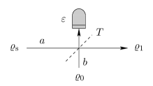
Figure 1: Scheme of the IPS process: the input state $\varrho_{\rm s}$ is mixed with the vacuum state $\varrho_{0}=|0\rangle\langle 0|$ at a beam splitter (BS) with transmissivity $T$; then, on/off photodetection with quantum efficiency $\varepsilon$ is performed on the reflected beam. When the detector clicks we obtain the IPS state $\varrho_{1}$

The scheme of the IPS process is sketched in figure 1. The mode $a$, excited in the state $\varrho_{\rm s}$ is mixed with the vacuum $\varrho_{0}=|0\rangle\langle 0|$ (mode $b$) at an unbalanced beam splitter (BS) with transmissivity $T=\cos^{2}\phi$ and then, on/off avalanche photodetection with quantum efficiency $\varepsilon$ is performed on the reflected beam. APDs can only discriminate the presence of radiation from the vacuum. The positive operator-valued measure (POVM) $\{\Pi_{0}(\varepsilon),\Pi_{1}(\varepsilon)\}$ of the detector is given by

$$\Pi_{0}(\varepsilon)=\sum_{k=0}^{\infty}(1-\varepsilon)^{k}\>|k\rangle\langle k|\,,\qquad\Pi_{1}(\varepsilon)={\mathbb{I}}-\Pi_{0}(\varepsilon)\;.$$ (1)

The whole process can be characterized by $T$ and $\varepsilon$ which will be referred to as the IPS transmissivity and the IPS quantum efficiency. The conditional state of the transmitted mode after the observation of a click is given by

$$\varrho_{1}=\frac{1}{p_{1}(\phi,\varepsilon)}\hbox{Tr}_{b}\left[U_{ab}(\phi)\varrho_{\rm s}\otimes\varrho_{0}\,U_{ab}^{{\dagger}}(\phi)\>{\mathbb{I}}_{a}\otimes\Pi_{1}(\varepsilon)\right]\;,$$ (2)

where $U_{ab}(\phi)=\exp\{-\phi(a^{{\dagger}}b-ab^{{\dagger}})\}$ is the evolution operator of the beam splitter, and $p_{1}(\phi,\varepsilon)$ is the probability of a click. In general, the transformation (2) realizes a non unitary quantum operation $\varrho_{1}=\mathcal{E}(\varrho_{\rm s})$ with operator-sum decomposition given by

$$\mathcal{E}(\varrho_{\rm s})=\frac{1}{p_{1}(\phi,\varepsilon)}\>\sum_{p=1}^{\infty}\>m_{p}(\phi,\varepsilon)\>E_{p}(\phi)\>\varrho_{\rm s}\>E_{p}^{{\dagger}}(\phi)\>\;$$ (3)

where

$$m_{p}(\phi,\varepsilon)={\displaystyle\frac{\tan^{2p}\phi\,\,[1-(1-\varepsilon)^{p}]}{p!}}\,,$$ (4)

$$M_{p}(\phi)=a^{p}\,\cos^{a^{\dagger}a}\phi\,.$$ (5)

which is found by explicit evaluation of the partial trace in (2). The IPS state obtained by applying the map (3) to a Gaussian state is no longer Gaussian, and therefore IPS represents an effective source of non Gaussian states, which should be otherwise generated by highly nonlinear, and thus inherently low rate, optical processes.

In general the IPS process can produce an output state whose energy is larger than the one of the input state and whose nonclassical properties can be enhanced. As an example, we address the photon subtraction onto a Gaussian state described by the following Wigner function (using the Wigner function formalism makes analytical calculations more straightforward):

$$W_{\rm s}(z)=\frac{\exp\{-F|z|^{2}-G(z^{2}+{z^{*}}^{2})\}}{\pi\sqrt{(F^{2}-4G^{2})^{-1}}}\,,$$ (6)

whose energy is given by

$$E_{\rm s}=\int_{\mathbb{C}}d^{2}z\,\left(|z|^{2}-\frac{1}{2}\right)\,W_{\rm s}(z)=\frac{F}{F^{2}-4G^{2}}-\frac{1}{2}\,.$$ (7)

When the state (6) undergoes the IPS process described above, the Wigner function associated with the output state $\varrho_{1}$ reads fock:oli

$$W_{1}(z)=\frac{1}{p_{1}(\phi,\varepsilon)}\,\sum_{k=1}^{2}\mathcal{C}_{k}(\phi,\varepsilon)\,W_{k}(z)\,,$$ (8)

with $\mathcal{C}_{1}(\phi,\varepsilon)=1$, $\mathcal{C}_{2}(\phi,\varepsilon)=-(\varepsilon\sqrt{{\rm Det}[{\boldsymbol{B}}+\boldsymbol{\sigma}_{\rm M}]})^{-1}$, where

$${\boldsymbol{B}}=(1-T)\boldsymbol{\sigma}+\frac{T}{2}\mathbbm{1}_{2}\,,\quad\boldsymbol{\sigma}_{\rm M}=\frac{2-\varepsilon}{2\varepsilon}\,\mathbbm{1}_{2}\,,$$ (9)

$\mathbbm{1}_{2}$ being the $2\times 2$ identity matrix, and $\boldsymbol{\sigma}$ is covariance associated with the state (6)

$$\boldsymbol{\sigma}=\left(\begin{array}[]{cc}(F+2G)^{-1}&0\\ 0&(F-2G)^{-1}\end{array}\right)\,,$$ (10)

where $[\boldsymbol{\sigma}]_{hk}=\frac{1}{2}\langle\{R_{h},R_{k}\}\rangle-\langle R_{h}\rangle\langle R_{k}\rangle$, $\{A,B\}=AB+BA$ denotes the anticommutator, and

$$\boldsymbol{R}=(R_{1},R_{2})^{T}\equiv\left(\frac{a+a^{{\dagger}}}{\sqrt{2}},\frac{a-a^{{\dagger}}}{i\sqrt{2}}\right)^{T}\,,$$ (11)

$(\cdots)^{T}$ being the transposition operation. Notice that $W_{1}(z)$ is no longer Gaussian. In Eq. (8) we defined

$$W_{k}(z)=\frac{\exp\{-F_{k}|z|^{2}-G_{k}(z^{2}+{z^{*}}^{2})\}}{\pi\sqrt{(F_{k}^{2}-4G_{k}^{2})^{-1}}}\,,$$ (12)

where

$$F_{1}=\mathcal{U}_{+}+\mathcal{U}_{-}\,,\quad G_{1}=\frac{1}{2}(\mathcal{U}_{+}-\mathcal{U}_{-})\,,$$ (13)

$$F_{2}=2(\mathcal{V}_{+}+\mathcal{V}_{-})\,,\quad G_{2}=\mathcal{V}_{+}-\mathcal{V}_{-}\,,$$ (14)

with

$$\mathcal{U}_{\pm}=\frac{F\pm 2G}{2T+(1-T)(F\pm 2G)}\,,$$ (15)

$$\mathcal{V}_{\pm}=\frac{F+2(1\pm G)T}{4T+(1-T)[2\varepsilon+(2-\varepsilon)(F\pm 2G)]\}}\,.$$ (16)

Because of the analytical expression (8), the energy of the photon subtracted state is simply given by

$$E_{1}(T,\varepsilon)=\frac{1}{p_{1}(T,\varepsilon)}\,\sum_{k=1}^{2}\mathcal{C}_{k}\,\left[\frac{F_{k}}{F_{k}^{2}-4G_{k}^{2}}-\frac{1}{2}\right]\,,$$ (17)

with $\mathcal{C}_{k}\equiv\mathcal{C}_{k}(T,\varepsilon)$ and where we put $T=\cos^{2}\phi$.

Figure 2: Logarithmic plots of the energies $E_{\rm s}$ (dashed line) and $E_{1}$ (solid lines) in the case of a squeezed vacuum $|0,r\rangle$ as input state and as functions of $\tanh r$ for $\varepsilon=1$ and different values of $T$. From top to bottom (solid lines): $T=1$, $0.9$, $0.75$, and $0.5$.

Figure 3: Plots of the energy $E_{1}$ of the IPS state in the case of a squeezed vacuum $|0,r\rangle$ as input state as a function of $\tanh r$ for $T=0.9$ (solid lines) and $T=0.8$ (dashed lines) and different values of $\varepsilon$. From top to bottom: $\varepsilon=1$, $0.75$, $0.5$, and $0.25$.

Let us now focus our attention on the IPS process applied to the squeezed vacuum $|0,r\rangle=S(r)|0\rangle$, $S(r)=\exp\{\frac{1}{2}r({a^{{\dagger}}}^{2}-a^{2})\}$ being the squeezing operator, which has been recently realized experimentally weng:PRL:04 . The Wigner function associated with $|0,r\rangle$ is given by Eq. (6) with $F=2\cosh 2r$ and $G=-\sinh 2r$. In Figs. 2 we plot the energies $E_{\rm s}$ and $E_{1}$ of the input and output states, respectively, for different values of the involved parameters as functions of $\tanh r$. We can see that there is a threshold on $r$, depending on $T$ and $\varepsilon$, under which the IPS state has a larger energy than the input state. Furthermore, when $\varepsilon=1$, $T\to 1$ and $r\to 0$ we can see that $E_{1}\to 1$: in these limits the output state approaches to the squeezed Fock state $S(r)|1\rangle$ jeong ; fock:oli . Finally, in Fig. 3 $E_{1}$ is plotted for two values of $T$ and different values of $\varepsilon$ as a function of $\tanh r$: we find that as $r$ increases, the IPS efficiency is not so relevant in the process.

III Photon subtraction on bipartite states

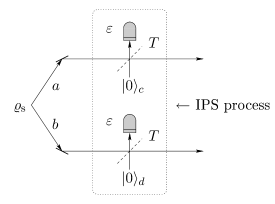
Figure 4: Scheme of the IPS process. The two modes, $a$ and $b$, of a shared bipartite state $\varrho_{\rm s}$ are mixed with the vacuum at two BSs with equal transmissivity $T$ and on/off photodetection with quantum efficiency $\varepsilon$ is performed on the reflected beam: when both the detectors click one obtains the IPS state.

In this Section we address de-Gaussification of bipartite states by IPS . The de-Gaussification can be achieved by subtracting photons from both modes through on/off detection ips:PRA:67 ; coch . The IPS scheme for two modes is sketched in Fig. 4. The modes $a$ and $b$ of the shared bipartite state $\varrho_{\rm s}$ are mixed with vacuum modes at two unbalanced beam splitters (BS) with equal transmissivity $T=\cos^{2}\phi$; the reflected modes $c$ and $d$ are then revealed by avalanche photodetectors (APD) with equal efficiency $\varepsilon$. The conditional measurement on modes $c$ and $d$, is described by the POVM (assuming equal quantum efficiency for the photodetectors)

$${\Pi}_{00}(\varepsilon) ={\Pi}_{0,c}(\varepsilon)\otimes{\Pi}_{0,d}(\varepsilon)\,,$$ (18)

$${\Pi}_{01}(\varepsilon) ={\Pi}_{0,c}(\varepsilon)\otimes{\Pi}_{1,d}(\varepsilon)\>,$$ (19)

$${\Pi}_{10}(\varepsilon) ={\Pi}_{1,c}(\varepsilon)\otimes{\Pi}_{0,d}(\varepsilon)\,,$$ (20)

$${\Pi}_{11}(\varepsilon) ={\Pi}_{1,c}(\varepsilon)\otimes{\Pi}_{1,d}(\varepsilon)\;.$$ (21)

When the two photodetectors jointly click, the conditioned output state of modes $a$ and $b$ is given by ips:PRA:67 ; ips:nonloc

$$\mathcal{E}(\varrho_{\rm s})=\frac{\hbox{Tr}_{cd}\big{[}U_{ac}(\phi)\otimes U_{bd}(\phi)\>\varrho_{\rm s}\otimes|0\rangle_{cd}{}_{dc}\langle 0|\>U_{ac}^{{\dagger}}(\phi)\otimes U_{bd}^{{\dagger}}(\phi)\>{\mathbb{I}}_{a}\otimes{\mathbb{I}}_{b}\otimes{\Pi}_{11}(\varepsilon)\big{]}}{p_{11}(r,\phi,\varepsilon)}\>,$$ (22)

where $U_{ac}(\phi)=\exp\{-\phi(a^{{\dagger}}c-ac^{{\dagger}})\}$ and $U_{bd}(\phi)$ are the evolution operators of the beam splitters, $|0\rangle_{cd}\equiv|0\rangle_{c}\otimes|0\rangle_{d}$, and $p_{11}(r,\phi,\varepsilon)$ is the probability of a click in both the detectors. The partial trace on modes $c$ and $d$ can be explicitly evaluated, thus arriving at the following decomposition of the IPS map:

$$\mathcal{E}(\varrho_{\rm s})=\frac{1}{p_{11}(r,\phi,\varepsilon)}\>\\ \times\sum_{p,q=1}^{\infty}\>m_{p}(\phi,\varepsilon)\>M_{pq}(\phi)\>\varrho_{\rm s}\>M_{pq}^{{\dagger}}(\phi)\>m_{q}(\phi,\varepsilon)\>$$ (23)

where

$$M_{pq}(\phi)=\frac{\mbox{}}{\mbox{}}a^{p}b^{q}\,(\cos\phi)^{a^{\dagger}a+b^{\dagger}b}\,.$$ (24)

Eq. (23) is indeed an operator-sum representation of the IPS map: $\{p,q\}\equiv\theta$ should be intended as a polyindex so that (23) reads $\mathcal{E}(\varrho_{\rm s})=\sum_{\theta}A_{\theta}\varrho_{\rm s}A^{\dagger}_{\theta}$ with $A_{\theta}=[p_{11}(r,\phi,\varepsilon)]^{-1/2}\,m_{p}(\phi,\varepsilon)\>M_{pq}(\phi)$.

From now on we focus our attention on the case in which the shared state is the twin-beam state of radiation (TWB) $\varrho_{\rm s}=|\Lambda\rangle\rangle\langle\langle\Lambda|$, where $|\Lambda\rangle\rangle=\sqrt{1-\lambda^{2}}\sum_{k}\lambda^{k}|k\rangle\otimes|k\rangle$ with $\lambda=\tanh r$, $r$ being the TWB squeezing parameter. The TWB is obtained by parametric down-conversion of the vacuum, $|\Lambda\rangle\rangle=\exp\{r(a^{\dagger}b^{\dagger}-ab)\}|0\rangle$, $a$ and $b$ being field operators, and it is described by the Gaussian Wigner function

$$W_{0}(\alpha,\beta)=\frac{\exp\{-2\widetilde{A}_{0}(|\alpha|^{2}+|\beta|^{2})+2\widetilde{B}_{0}(\alpha\beta+\alpha^{*}\beta^{*})\}}{\pi^{2}\sqrt{{\rm Det}[\boldsymbol{\sigma}_{0}]}}\,,$$ (25)

with

$$\widetilde{A}_{0}=\frac{A_{0}}{4\sqrt{{\rm Det}[\boldsymbol{\sigma}_{0}]}}\,,\qquad\widetilde{B}_{0}=\frac{B_{0}}{4\sqrt{{\rm Det}[\boldsymbol{\sigma}_{0}]}}\,,$$ (26)

where $A_{0}\equiv A_{0}(r)=\cosh(2r)$, $B_{0}\equiv B_{0}(r)=\sinh(2r)$ and $\boldsymbol{\sigma}_{0}$ is the covariance matrix

$$\boldsymbol{\sigma}_{0}=\frac{1}{2}\left(\begin{array}[]{cc}A_{0}\,\mathbbm{1}_{2}&B_{0}\,\boldsymbol{\sigma}_{3}\\[4.30554pt] B_{0}\,\boldsymbol{\sigma}_{3}&A_{0}\,\mathbbm{1}_{2}\end{array}\right)\>,$$ (27)

$\mathbbm{1}_{2}$ being the $2\times 2$ identity matrix and $\boldsymbol{\sigma}_{3}={\rm Diag}(1,-1)$; $\boldsymbol{\sigma}_{0}$ is defined as $[\boldsymbol{\sigma}_{0}]_{hk}=\frac{1}{2}\langle\{R_{h},R_{k}\}\rangle-\langle R_{h}\rangle\langle R_{k}\rangle$ with

$$\boldsymbol{R} =(R_{1},R_{2},R_{3},R_{4})^{T}$$ (28)

$$\equiv\left(\frac{a+a^{{\dagger}}}{\sqrt{2}},\frac{a-a^{{\dagger}}}{i\sqrt{2}},\frac{b+b^{{\dagger}}}{\sqrt{2}},\frac{b-b^{{\dagger}}}{i\sqrt{2}}\right)^{T}\,.$$ (29)

Now we explicitly calculate the Wigner function of the corresponding IPS state, which, as one may expect, is no longer Gaussian and positive-definite. The state entering the two beam splitters is described by the Wigner function

$$W_{0}^{\hbox{\tiny(in)}}(\alpha,\beta,\zeta,\xi)=W_{0}(\alpha,\beta)\,\frac{4}{\pi^{2}}\exp\left\{-2|\zeta|^{2}-2|\xi|^{2}\right\}\,,$$ (30)

where the second factor at the right hand side represents the two vacuum states of modes $c$ and $d$. The action of the beam splitters on $W^{\hbox{\tiny(in)}}_{r}$ can be summarized by the following change of variables FOP:napoli:05

$$\alpha\to\alpha\cos\phi+\zeta\sin\phi\,, \zeta\to\zeta\cos\phi-\alpha\sin\phi\,,$$ (31)

$$\beta\to\beta\cos\phi+\xi\sin\phi\,, \xi\to\xi\cos\phi-\beta\sin\phi\,,$$ (32)

and the output state, after the beam splitters, is then given by

$$W_{r,\phi}^{\hbox{\tiny(out)}}(\alpha,\beta,\zeta,\xi)=\\ \frac{4}{\pi^{2}}\,W_{r,\phi}(\alpha,\beta)\,\exp\left\{-a|\xi|^{2}+w\xi+w^{*}\xi^{*}\right\}\\ \times\exp\big{\{}-a|\zeta|^{2}+(v+2\widetilde{B}_{0}\xi\sin^{2}\phi)\zeta\\ +(v^{*}+2\widetilde{B}_{0}\xi^{*}\sin^{2}\phi)\zeta^{*}\big{\}}\,,$$ (33)

where

$$W_{r,\phi}(\alpha,\beta)=\\ \frac{\exp\{-b(|\alpha|^{2}+|\beta|^{2})+2\widetilde{B}_{0}\cos^{2}\phi\,(\alpha\beta+\alpha^{*}\beta^{*})\}}{\pi^{2}\sqrt{{\rm Det}[\boldsymbol{\sigma}_{0}]}}$$ (34)

and

$$a\equiv a(r,\phi)=2(\widetilde{A}_{0}\sin^{2}\phi+\cos^{2}\phi),$$ (35)

$$b\equiv b(r,\phi)=2(\widetilde{A}_{0}\cos^{2}\phi+\sin^{2}\phi)\,,$$ (36)

$$v\equiv v(r,\phi)=2\cos\phi\,\sin\phi\,[(1-\widetilde{A}_{0})\alpha^{*}+\widetilde{B}_{0}\beta],$$ (37)

$$w\equiv w(r,\phi)=2\cos\phi\,\sin\phi\,[(1-\widetilde{A}_{0})\beta^{*}+\widetilde{B}_{0}\alpha]\,.$$ (38)

At this stage on/off detection is performed on modes $c$ and $d$ (see Fig. 4). We are interested in the situation when both the detectors click. The Wigner function of the double click element $\Pi_{11}(\varepsilon)$ of the POVM [see Eq. (21)] is given by ips:PRA:67 ; cond:cola

$$W_{\varepsilon}(\zeta,\xi) \equiv W[\Pi_{11}(\varepsilon)](\zeta,\xi)$$ (39)

$$=\frac{1}{\pi^{2}}\{1-Q_{\varepsilon}(\zeta)-Q_{\varepsilon}(\xi)+Q_{\varepsilon}(\zeta)Q_{\varepsilon}(\xi)\}\,,$$ (40)

with

$$Q_{\varepsilon}(z)=\frac{2}{2-\varepsilon}\,\exp\Bigg{\{}-\frac{2\varepsilon}{2-\varepsilon}\,|z|^{2}\Bigg{\}}\,.$$ (41)

Using Eq. (22) and the phase-space expression of trace for each mode, i.e.,

$${\rm Tr}[O_{1}\,O_{2}]=\pi\int_{\mathbb{C}}d^{2}z\,W[O_{1}](z)\,W[O_{2}](z)\,,$$ (42)

the Wigner function of the output state, conditioned to the double click event, reads

$$W_{r,\phi,\varepsilon}(\alpha,\beta)=\frac{f(\alpha,\beta)}{p_{11}(r,\phi,\varepsilon)}\,,$$ (43)

where $f(\alpha,\beta)\equiv f_{r,\phi,\varepsilon}(\alpha,\beta)$ with

$$f(\alpha,\beta)=\pi^{2}\,\int_{\mathbb{C}^{2}}d^{2}\zeta\,d^{2}\xi\,\frac{4}{\pi^{2}}\,W_{r,\phi}(\alpha,\beta)\,\\ \times\sum_{k=1}^{4}\frac{C_{k}}{\pi^{2}}\,G_{r,\phi,\varepsilon}^{(k)}(\alpha,\beta,\zeta,\xi)\,,$$ (44)

with $C_{k}\equiv C_{k}(\varepsilon)$ and $C_{1}=1$, $C_{2}=C_{3}=-2(2-\varepsilon)^{-1}$, $C_{4}=4(2-\varepsilon)^{-2}$; the double-click probability $p_{11}(r,\phi,\varepsilon)$ can be written as function of $f(\alpha,\beta)$ as follows

$$p_{11}(r,\phi,\varepsilon)=\pi^{2}\,\int_{\mathbb{C}^{2}}d^{2}\alpha\,d^{2}\beta\,f(\alpha,\beta)\,.$$ (45)

The quantities $G_{r,\phi,\varepsilon}^{(k)}(\alpha,\beta,\zeta,\xi)$ in Eq. (44) are given by

$$G_{r,\phi,\varepsilon}^{(k)}(\alpha,\beta,\zeta,\xi)=\\ \exp\big{\{}-x_{k}|\zeta|^{2}+(v+2B\xi\sin^{2}\phi)\zeta\\ +(v^{*}+2B\xi^{*}\sin^{2}\phi)\zeta^{*}\big{\}}\\ \times\exp\left\{-y_{k}|\xi|^{2}+w\xi+w^{*}\xi^{*}\right\}\,,$$ (46)

where $x_{k}\equiv x_{k}(r,\phi,\varepsilon)$, and $y_{k}\equiv y_{k}(r,\phi,\varepsilon)$ are

$$x_{1}=x_{3}=y_{1}=y_{2}=a$$

$$x_{2}=x_{4}=y_{3}=y_{4}=a+2\varepsilon(2-\varepsilon)^{-1}\,.$$

After the integrations we have

$$f(\alpha,\beta)=\frac{1}{\pi^{2}}\,\sum_{k=1}^{4}{\cal C}_{k}\,\exp\{(f_{k}-b)|\alpha|^{2}+(g_{k}-b)|\beta|^{2}\\ +(2\widetilde{B}_{0}T+h_{k})(\alpha\beta+\alpha^{*}\beta^{*})\}$$ (47)

and

$$p_{11}(r,T,\varepsilon)=\sum_{k=1}^{4}\frac{{\cal C}_{k}}{(b-f_{k})(b-g_{k})-(2\widetilde{B}_{0}T+h_{k})^{2}}\,,$$ (48)

where we put $T=\cos^{2}\phi=1-\sin^{2}\phi$, and defined

$${\cal C}_{k}\equiv{\cal C}_{k}(r,T,\varepsilon)=\frac{4C_{k}}{[x_{k}y_{k}-4\widetilde{B}_{0}^{2}(1-T)^{2}]\sqrt{{\rm Det}[\boldsymbol{\sigma}_{0}]}}$$ (49)

and $f_{k}\equiv f_{k}(r,T)$, $g_{k}\equiv g_{k}(r,T)$, and $h_{k}\equiv h_{k}(r,T)$ given by

$$f_{k}={\cal N}_{k}\,[x_{k}\widetilde{B}_{0}^{2}+4\widetilde{B}_{0}^{2}(1-\widetilde{A}_{0})(1-T)+y_{k}(1-\widetilde{A}_{0})^{2}]\,,$$ (50)

$$g_{k}={\cal N}_{k}\,[x_{k}(1-\widetilde{A}_{0})^{2}+4\widetilde{B}_{0}^{2}(1-\widetilde{A}_{0})(1-T)+y_{k}\widetilde{B}_{0}^{2}]\,,$$ (51)

$$h_{k}={\cal N}_{k}\,\{(x_{k}+y_{k})\widetilde{B}_{0}(1-\widetilde{A}_{0})$$

$$\hskip 56.9055pt+2\widetilde{B}_{0}[\widetilde{B}_{0}^{2}+(1-\widetilde{A}_{0})^{2}](1-T)\}\,,$$ (52)

$${\cal N}_{k}\equiv{\cal N}_{k}(r,T)={\displaystyle\frac{4T\,(1-T)}{x_{k}y_{k}-4\widetilde{B}_{0}^{2}(1-T)^{2}}\,.}$$ (53)

In this way, the Wigner function of the IPS state can be rewritten as

$$W_{\hbox{\rm\tiny IPS}}(\alpha,\beta)=\frac{1}{\pi^{2}\,p_{11}(r,T,\varepsilon)}\sum_{k=1}^{4}{\cal C}_{k}\,W_{k}(\alpha,\beta)\,,$$ (54)

with

$$W_{k}(\alpha,\beta)=\exp\{(f_{k}-b)|\alpha|^{2}+(g_{k}-b)|\beta|^{2}\\ +(2\widetilde{B}_{0}T+h_{k})(\alpha\beta+\alpha^{*}\beta^{*})\}\,.$$ (55)

Finally, the density matrix corresponding to $W_{\hbox{\rm\tiny IPS}}(\alpha,\beta)$ reads as follows ips:PRA:67

$${\varrho}_{\hbox{\rm\tiny IPS}}=\frac{1-\lambda^{2}}{p_{11}(r,T,\varepsilon)}\sum_{n,m=0}^{\infty}(\lambda T)^{n+m}\sum_{h,k=0}^{{\rm Min}[n,m]}{\cal A}_{h,k}(T,\varepsilon)\\ \times\sqrt{\frac{n}{h}\frac{n}{k}\frac{m}{h}\frac{m}{k}}\,|n-k\rangle_{a}|n-h\rangle_{b}{{}_{b}}\langle m-h|{{}_{a}}\langle m-k|\,,$$ (56)

where $\lambda=\tanh r$ and

$${\cal A}_{h,k}(T,\varepsilon)=\left[1-(1-\varepsilon)^{h}\right]\left[1-(1-\varepsilon)^{k}\right]\left(\frac{1-T}{T}\right)^{h+k}\>.$$ (57)

Figure 5: Logarithmic plots of the energies $E_{\rm s}$ (dashed line) and $E_{\hbox{\rm\tiny IPS}}$ (solid lines) in the case of a TWB as input state as functions of $\tanh r$ for $\varepsilon=1$ and different values of $T$. From top to bottom (solid lines): $T=1$, $0.9$, $0.75$, and $0.5$.

Figure 6: Plots of the energy $E_{\hbox{\rm\tiny IPS}}$ of the IPS state in the case of the TWB as input state as a function of $\tanh r$ for $T=0.9$ (solid lines) and $T=0.8$ (dashed lines) and different values of $\varepsilon$. From top to bottom: $\varepsilon=1$, $0.75$, $0.5$, and $0.25$.

In Fig. 5 we plot the energies $E_{\rm s}$ and $E_{\hbox{\rm\tiny IPS}}$ of the bipartite input and output states, respectively, for different values of the involved parameters as functions of $\tanh r$. We recall that for a given Wigner function $W(v,w)$ of a bipartite state, the corresponding energy is

$$E=\int_{\mathbb{C}^{2}}d^{2}v\,d^{2}w\,\left(|v|^{2}+|w|^{2}-1\right)\,W(v,w)\,.$$ (58)

If the bipartite state has a Wigner function of the form

$$W_{\rm s}(v,w)=\frac{\exp\{-F|v|^{2}-G|w|^{2}+H(vw+v^{*}w^{*})\}}{\pi^{2}(FG-H^{2})^{-1}}\,,$$ (59)

then its energy reads:

$$E_{\rm s}=\frac{F+G}{2(FG-H^{2})}-1\,;$$ (60)

thereby, in the case of a TWB as input state $F$, $G$, and $H$ are obtained from Eq. (25) and the energy of the state emerging from the IPS process can be written as

$$E_{\hbox{\rm\tiny IPS}}=\frac{1}{\pi^{2}\,p_{11}(r,T,\varepsilon)}\sum_{k=1}^{4}{\cal C}_{k}\left[\frac{F_{k}+G_{k}}{2(F_{k}G_{k}-H_{k}^{2})^{2}}-1\right]\,$$ (61)

with $F_{k}=b-f_{h}$, $G_{k}=b-g_{h}$, and $H_{k}=2\widetilde{B}_{0}T+h_{k}$ and all the involved quantities are the same as in Eq. (54). As in the single mode case, we can see that there is a threshold on $r$, depending on $T$ and $\varepsilon$, under which the IPS state has a larger energy than the input state. In Fig. 6 $E_{\hbox{\rm\tiny IPS}}$ is plotted for two values of $T$ and different values of $\varepsilon$ as a function of $\tanh r$: we find that as $r$ decreases, the IPS efficiency is not so relevant.

The state given in Eq. (54) is no longer a Gaussian state and its use in the improvement of continuous variable teleportation ips:PRA:67 as well as in the enhancement of the nonlocality ips:nonloc ; nha ; sanchez will be investigated in the following Sections.

IV Dynamics of TWB in noisy channels

Before addressing the properties of the IPS bipartite state described in the previous Section, we review the evolution of the twin-beam state of radiation (TWB) in a noisy environment, namely, an environment where dissipation and thermal noise take place OP:PSnoise . As we will see, we can include in our analysis the effect due to the propagation through this kind of channel by a simple change of the involved quantities. Using a more compact form, Eq. (25) can also be rewritten as

$$W_{0}(\boldsymbol{X})=\frac{\exp\left\{-\frac{1}{2}\,\boldsymbol{X}^{T}\,\boldsymbol{\sigma}_{0}^{-1}\,\boldsymbol{X}\right\}}{\pi^{2}\sqrt{{\rm Det}[\boldsymbol{\sigma}_{0}]}}\,,$$ (62)

with $\boldsymbol{X}=(x_{1},y_{1},x_{2},y_{2})^{T}$, $\alpha=\frac{1}{\sqrt{2}}(x_{1}+iy_{1})$ and $\beta=\frac{1}{\sqrt{2}}(x_{2}+iy_{2})$, and $(\cdots)^{T}$ denoting the transposition operation.

When the two modes of the TWB interact with a noisy environment, namely in the presence of dissipation and thermal noise, the evolution of the Wigner function (25) is described by the following Fokker-Planck equation wm:quantopt:94 ; binary ; seraf:PRA:69

$$\partial_{t}W_{t}(\boldsymbol{X})=\frac{1}{2}\Big{(}\partial_{\boldsymbol{X}}^{T}{\rm I}\!\Gamma\boldsymbol{X}+\partial_{\boldsymbol{X}}^{T}{\rm I}\!\Gamma\boldsymbol{\sigma}_{\infty}\partial_{\boldsymbol{X}}\Big{)}W_{t}(\boldsymbol{X})\,,$$ (63)

with $\partial_{\boldsymbol{X}}=(\partial_{x_{1}},\partial_{y_{1}},\partial_{x_{2}},\partial_{y_{2}})^{T}$. The damping matrix is given by ${\rm I}\!\Gamma=\bigoplus_{k=1}^{2}\,\Gamma_{k}\mathbbm{1}_{2}$, whereas

$$\boldsymbol{\sigma}_{\infty} =\bigoplus_{k=1}^{2}\,\boldsymbol{\sigma}_{\infty}^{(k)}=\left(\begin{array}[]{cc}\boldsymbol{\sigma}_{\infty}^{(1)}&\boldsymbol{0}\\[4.30554pt] \boldsymbol{0}&\boldsymbol{\sigma}_{\infty}^{(2)}\end{array}\right)\,,$$ (66)

where $\boldsymbol{0}$ is the $2\times 2$ null matrix and

$$\boldsymbol{\sigma}_{\infty}^{(k)}=\frac{1}{2}\left(\begin{array}[]{cc}1+2N_{k}&0\\[4.30554pt] 0&1+2N_{k}\end{array}\right)\,.$$ (67)

$\Gamma_{k}$, $N_{k}$ denote the damping rate and the average number of thermal photons of the channel $k$, respectively. $\boldsymbol{\sigma}_{\infty}$ represents the covariance matrix of the environment and, in turn, the asymptotic covariance matrix of the evolved TWB. Since the environment is itself excited in a Gaussian state, the evolution induced by (63) preserves the Gaussian form (62). The covariance matrix at time $t$ reads as follows seraf:PRA:69 ; FOP:napoli:05

$$\boldsymbol{\sigma}_{t}=\mathbbm{G}_{t}^{1/2}\,\boldsymbol{\sigma}_{0}\,\mathbbm{G}_{t}^{1/2}+(\mathbbm{1}-\mathbbm{G}_{t})\,\boldsymbol{\sigma}_{\infty}\,,$$ (68)

where $\mathbbm{G}_{t}=\bigoplus_{k=1}^{2}\,e^{-\Gamma_{k}t}\,\mathbbm{1}_{2}$. The covariance matrix $\boldsymbol{\sigma}_{t}$ can be also written as

$$\boldsymbol{\sigma}_{t}=\frac{1}{2}\left(\begin{array}[]{cc}A_{t}(\Gamma_{1},N_{1})\,\mathbbm{1}_{2}&B_{t}(\Gamma_{1})\,\boldsymbol{\sigma}_{3}\\[4.30554pt] B_{t}(\Gamma_{2})\,\boldsymbol{\sigma}_{3}&A_{t}(\Gamma_{2},N_{2})\,\mathbbm{1}_{2}\end{array}\right)$$ (69)

with

$$\begin{array}[]{l}A_{t}(\Gamma_{k},N_{k})=A_{0}\,e^{-\Gamma_{k}t}+\left(1-e^{-\Gamma_{k}t}\right)(1+2N_{k})\,,\\[4.30554pt] B_{t}(\Gamma_{k})=B_{0}\,e^{-\Gamma_{k}t}\,.\end{array}$$ (70)

Finally, if we assume $\Gamma_{1}=\Gamma_{2}=\Gamma$ and $N_{1}=N_{2}=N$, then the covariance matrix (69) becomes formally identical to (27) and the corresponding Wigner function reads

$$W_{t}(\alpha,\beta)=\frac{\exp\{-2\widetilde{A}_{t}(|\alpha|^{2}+|\beta|^{2})+2\widetilde{B}_{t}(\alpha\beta+\alpha^{*}\beta^{*})\}}{\pi^{2}\sqrt{{\rm Det}[\boldsymbol{\sigma}_{t}]}}\,,$$ (71)

with

$$\widetilde{A}_{t}=\frac{A_{t}(\Gamma,N)}{4\sqrt{{\rm Det}[\boldsymbol{\sigma}_{t}]}}\,,\qquad\widetilde{B}_{t}=\frac{B_{t}(\Gamma)}{4\sqrt{{\rm Det}[\boldsymbol{\sigma}_{t}]}}\,.$$ (72)

If the IPS process is performed on a TWB evolved in a noisy environment with both the channels having the same damping rate and thermal noise, then the Wigner function of the state arriving at the beam splitters is now given by Eq. (71), and the output state is still described by Eq. (54), but with the following substitutions

$$\widetilde{A}_{0}\to\widetilde{A}_{t}\,,\quad\widetilde{B}_{0}\to\widetilde{B}_{t}\,,\quad\boldsymbol{\sigma}_{0}\to\boldsymbol{\sigma}_{t}\,.$$ (73)

V Continuous variable teleportation

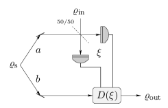
Figure 7: Scheme of the CV teleportation. One of the two modes of a shared bipartite state $\varrho_{\rm s}$ is mixed with the input state $\varrho_{\rm in}$ at a balanced BS, and then a double homodyne detection is performed on the two output modes measuring the complex outcome $\xi$. The teleported state $\varrho_{\rm out}$ is obtained displacing by the same amount $\xi$ the remaining mode of the shared state and averaging over all the possible outcomes.

The scheme of continuous variable (CV) teleportation is sketched in Fig. 7. A bipartite state $W_{\rm s}$ is shared between two parties: one mode of the state is mixed at a balanced beam splitter (BS) with the state to be teleported, $W_{\rm in}$, then double-homodyne measurement is performed on the two emerging modes. The complex outcome $\xi$ of the measurement is used in order to displace the remaining mode of $W_{\rm s}$ and the teleported state $W_{\rm out}$ is obtained averaging over all the possible outcomes. Here we address the teleportation of the coherent state $|\alpha\rangle$, whose Wigner function reads

$$W_{\rm in}(z)=\frac{2}{\pi}\exp\{-2|z-\alpha|^{2}\}\,.$$ (74)

If we consider the following generic shared state:

$$W_{\rm s}(v,w)=\frac{\exp\{-F|v|^{2}-G|w|^{2}+H(vw+v^{*}w^{*})\}}{\pi^{2}(FG-H^{2})^{-1}}\,,$$ (75)

and since the POVM describing the double homodyne detection is

$$W_{\xi}(z,v)=\frac{1}{\pi^{2}}\,\delta^{(2)}(z-v^{*}-\xi)\,,$$ (76)

$\delta^{(2)}(\zeta)$ being the complex Dirac’s delta function, the output state $W_{\rm out}$ is given by FOP:napoli:05

$$W_{{\rm out}}(w) =\pi^{2}\int_{\mathbb{C}}d^{2}\xi\int_{{\mathbb{C}}^{2}}d^{2}z\,d^{2}v\,W_{\rm in}(z)\,$$

$$\hskip 56.9055pt\times\,W_{\rm s}(v,w-\xi)\,W_{\xi}(z,v)$$ (77)

$$=\frac{1}{\pi\sigma_{\rm out}}\exp\left\{-\frac{|w-\alpha|^{2}}{\sigma_{\rm out}}\right\}\,,$$ (78)

where

$$\sigma_{\rm out}=\frac{1}{2}+\frac{F+G+2H}{FG-H^{2}}\,;$$ (79)

in turn, the average fidelity of teleportation of coherent states reads as follows:

$$\overline{F} \equiv\pi\int_{\mathbb{C}}d^{2}w\,W_{\rm in}(w)\,W_{\rm out}(w)$$ (80)

$$=\frac{FG-H^{2}}{FG-H^{2}+F+G-2H}=\frac{2}{1+2\,\sigma_{\rm out}}\,.$$ (81)

When the shared state is the TWB of Eq. (25), the average fidelity is obtained from Eq. (80) with $F=G=2\widetilde{A}_{0}$ and $H=2\widetilde{B}_{0}$, i.e.,

$$\overline{F}_{\hbox{\tiny TWB}}(\lambda)=\mbox{$\frac{1}{2}$}(1+\lambda)$$ (82)

whereas in the presence of noise one should use the substitutions (73). $\overline{F}_{\hbox{\tiny TWB}}$ is plotted in Fig. 8.

Figure 8: Plots of the teleportation fidelity $\overline{F}_{\mbox{\tiny TWB}}$ assisted by TWB in the ideal case ($\Gamma t=N=0$, dot-dashed line) as a function of $\lambda=\tanh r$. The solid lines are $\overline{F}_{\mbox{\tiny TWB}}$ with $\Gamma t=0.2$ and, from top to bottom, $N=0$, $0.1$, $0.2$, and $0.5$.

When the teleportation is assisted by IPS, then the fidelity reads as follows:

$$\overline{F}_{\hbox{\tiny IPS}}=\frac{1}{p_{11}(r,T,\varepsilon)}\sum_{k=1}^{4}\frac{{\cal C}_{k}}{F_{k}G_{k}-H_{k}^{2}+F_{k}+G_{k}-2H_{k}}\,,$$ (83)

with $F_{k}=b-f_{h}$, $G_{k}=b-g_{h}$, and $H_{k}=2\widetilde{B}_{0}T+h_{k}$ and all the involved quantities are the same as in Eq. (54). The results are presented in Fig. 9 for $\varepsilon=1$ and $\Gamma t=N=0$. The IPS state improves the average fidelity of quantum teleportation when $\lambda$ is below a certain threshold, which depends on $T$ (and $\varepsilon$). Notice that, for $T<0.5$, $\overline{F}_{\hbox{\tiny IPS}}(\lambda)$ is always below $\overline{F}_{\hbox{\tiny TWB}}(\lambda)$, at least for $\varepsilon=1$.

Figure 9: Plots of the teleportation fidelity $\overline{F}_{\mbox{\tiny IPS}}$ assisted by IPS in the ideal case ($\Gamma t=N=0$) as a function of $\lambda=\tanh r$. The dashed line is $\overline{F}_{\mbox{\tiny TWB}}$, whereas the solid lines are $\overline{F}_{\mbox{\tiny IPS}}$ with $\varepsilon=1$ and, from top to bottom, $T=1.0$, $0.9$, $0.8$, and $0.5$.

The effect of dissipation and thermal noise is shown in Fig. 10.

Figure 10: Plots of the teleportation fidelity $\overline{F}_{\mbox{\tiny IPS}}$ assisted by IPS as a function of $\lambda=\tanh r$ with $T=0.9$, $\varepsilon=1$, $\Gamma t=0.1$ and different values of $N$ (solid lines): from top to bottom $N=0$, $0.1$, $0.2$, and $0.3$. The dot-dashed line is $\overline{F}_{\mbox{\tiny IPS}}$ with $T=0.9$, $\varepsilon=1$, and $\Gamma t=N=0$.

In order to quantify the improvement and to study its dependence on $T$ and $\varepsilon$, we define the following “relative improvement”:

$${\cal R}_{F}(r,T,\varepsilon,\Gamma,N)=\frac{\overline{F}_{\hbox{\tiny IPS}}(r,T,\varepsilon,\Gamma,N)-\overline{F}_{\hbox{\tiny TWB}}(r,\Gamma,N)}{\overline{F}_{\hbox{\tiny TWB}}(r,\Gamma,N)}\,,$$ (84)

which is plotted in Fig. 11: we can see that ${\cal R}_{F}$ and, in turn, $\overline{F}_{\hbox{\tiny IPS}}$ are mainly affected by $T$ when $\Gamma t$ and $N$ are fixed.

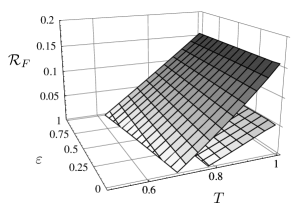
Figure 11: Plots of ${\cal R}_{F}$ as a function of $T$ and $\varepsilon$ with $r=0.3$; we set $\Gamma t=N=0$ (upper surface) and $\Gamma t=N=0.1$ (lower surface). ${\cal R}_{F}$, and, in turn, $\overline{F}_{\mbox{\tiny IPS}}$, is mainly affected by the IPS transmissivity $T$.

In Fig. 12 we plot ${\cal R}_{F}$ as a function $\lambda=\tanh r$ and the quantity ${\cal R}_{F}^{\rm(id)}$ defined as follows:

$${\cal R}_{F}^{\rm(id)}(r,T,\varepsilon,\Gamma,N)=\frac{\overline{F}_{\hbox{\tiny IPS}}(r,T,\varepsilon,\Gamma,N)-\overline{F}_{\hbox{\tiny TWB}}(r,0,0)}{\overline{F}_{\hbox{\tiny TWB}}(r,0,0)}\,,$$ (85)

i.e., the relative improvement of the fidelity using IPS in the presence of losses and thermal noise with respect to the fidelity using the TWB in ideal conditions ($\Gamma t=N=0$): we can see that, for the particular choice of the parameters, not only the fidelity is improved with respect the TWB-based teleportation in the presence of the same dissipation and thermal noise (solid line in Fig. 12), but the results can be also better than the ideal case (dot-dashed line). We can conclude that IPS onto TWB degraded by dissipation and noisy environment can improve the fidelity of teleportation up to and beyond the value achievable using the TWB in ideal conditions.

Figure 12: Plot of the relative enhancement ${\cal R}_{F}$ as a function of $\lambda=\tanh r$ with $T=0.9$, $\varepsilon=1$, and $\Gamma t=N=0.1$ (solid line). The dot-dashed line is ${\cal R}_{F}^{\rm(id)}$, namely, the relative enhancement of the fidelity using the de-Gaussified TWB in noisy environment with respect to the fidelity using TWB in ideal case (see text for details): for a suitable choice of the parameters, the teleportation assisted by IPS in the presence of dissipation and thermal noise, can have a fidelity larger than the one of TWB-assisted teleportation also when this is implemented in ideal conditions (i.e., $\Gamma t=N=0$).

Figure 13: Plot of the teleportation fidelity as a function of the average number of photons $N$ of the shared state in the case of TWB (dashed line) and a photon subtracted TWB (solid line) for $T=0.999$, $\varepsilon=1$, and in ideal conditions (i.e., $\Gamma t=N=0$. The inset is a magnification of the region $0<N<2$.

Finally, in Fig. 13 we plot the teleportation fidelity as a function of the average number of photons $N$ of the shared state in the case of TWB and a photon subtracted TWB: we can see that for a fixed energy of the shared quantum channel the best fidelity is achieved by the TWB state. The same result holds in the presence of dissipation and thermal noise.

In the next Sections we will analyze the nonlocality of the IPS state in the presence of noise by means of Bell’s inequalities OP:PSnoise .

VI Nonlocality in the phase space

Parity is a dichotomic variable and thus can be used to establish Bell-like inequalities CHSH . The displaced parity operator on two modes is defined as bana

$$\hat{\Pi}(\alpha,\beta)=D_{a}(\alpha)(-1)^{a^{\dagger}a}D_{a}^{\dagger}(\alpha)\otimes D_{b}(\beta)(-1)^{b^{\dagger}b}D_{b}^{\dagger}(\beta)\,,$$ (86)

where $\alpha,\beta\in{\mathbb{C}}$, $a$ and $b$ are mode operators and $D_{a}(\alpha)=\exp\{\alpha a^{\dagger}-\alpha^{*}a\}$ and $D_{b}(\beta)$ are single-mode displacement operators. Since the two-mode Wigner function $W(\alpha,\beta)$ can be expressed as FOP:napoli:05

$$W(\alpha,\beta)=\frac{4}{\pi^{2}}\,\Pi(\alpha,\beta)\,,$$ (87)

$\Pi(\alpha,\beta)$ being the expectation value of $\hat{\Pi}(\alpha,\beta)$, the violation of these inequalities is also known as nonlocality in the phase-space. The quantity involved in such inequalities can be written as follows

$${\cal B}_{\rm DP}=\Pi(\alpha_{1},\beta_{1})+\Pi(\alpha_{2},\beta_{1})+\Pi(\alpha_{1},\beta_{2})-\Pi(\alpha_{2},\beta_{2})\,,$$ (88)

which, for local theories, satisfies $|\mathcal{B}_{\rm DP}|\leq 2$.

Following Ref. bana , one can choose a particular set of displaced parity operators, arriving at the following combination ips:PRA:70

$${\cal B}_{\rm DP}({\cal J})=\Pi(\sqrt{\cal J},-\sqrt{\cal J})+\Pi(-3\sqrt{\cal J},-\sqrt{\cal J})\\ +\Pi(\sqrt{\cal J},3\sqrt{\cal J})-\Pi(-3\sqrt{J},3\sqrt{\cal J})\,,$$ (89)

which, for the TWB, gives a maximum ${\cal B}_{\rm DP}=2.32$ (for ${\cal J}=1.6\times 10^{-3}$) greater than the value $2.19$ obtained in Ref. bana . Notice that, even in the infinite squeezing limit, the violation is never maximal, i.e., $|\mathcal{B}_{\rm DP}|<2\sqrt{2}$ jeong1 .

In Ref. ips:PRA:70 we studied Eq. (89) for both the TWB and the IPS state in an ideal scenario, namely in the absence of dissipation and noise; we showed that, using IPS, the maximum violation is achieved for $T,\varepsilon\to 1$ and for values of $r$ smaller than for the TWB.

Figure 14: Plots of the Bell parameters ${\cal B}_{\rm DP}$ for the TWB (top) and IPS (bottom); we set ${\cal J}=1.6\times 10^{-3}$, which maximizes ${\cal B}_{\rm DP}^{\rm(TWB)}$, and put $T=0.9999$ and $\varepsilon=1$ for the IPS. The dashed lines refer to the absence of noise ($\Gamma t=N=0$), whereas, for both the plot, the solid lines are ${\cal B}_{\rm DP}$ with $\Gamma t=0.01$ and, from top to bottom, $N=0,0.05,0.1,$ and $0.2$. In the ideal case the maxima are ${\cal B}_{\rm DP}^{\rm(TWB)}=2.32$ and ${\cal B}_{\rm DP}^{\rm(IPS)}=2.43$, respectively.

Now, by means of the Eq. (54) and the substitutions (73), we can study how noise affects ${\cal B}_{\rm DP}$. The results are showed in Fig. 14 for $\varepsilon=1$: as one may expect, the overall effect of noise is to reduce the violation of the Bell’s inequality. When dissipation alone is present ($N=0$), the maximum of violation is achieved using the IPS for values of $r$ smaller than for the TWB, as in the ideal case. On the other hand, one can see that the presence of thermal noise mainly affects the IPS results. In fact, for $\Gamma t=0.01$ and $N=0.2$, one has $|{\cal B}_{\rm DP}^{\rm(TWB)}|>2$ for a range of $r$ values, whereas $|{\cal B}_{\rm DP}^{\rm(IPS)}|$ falls below the threshold for violation. Note that the maximum of violation, both for the TWB and the IPS state, depends on the squeezing parameter $r$.

Figure 15: The surfaces are plots of the Bell parameters ${\cal B}_{\rm DP}$ for the IPS state as a function of $T$ and $\varepsilon$ for different values of $\Gamma t$ and $N=0$: (top) $\Gamma t=0$; (bottom) $\Gamma t=0.005$. We set ${\cal J}=1.6\times 10^{-3}$ and $r=1.16$ The value of the Bell parameter is mainly affected by $T$.

In Fig. 15 we plot ${\cal B}_{\rm DP}^{\rm(IPS)}$ as a function of $T$ and $\varepsilon$. We can see that the main contribution to the Bell parameter is due to the transmissivity $T$. Moreover, as $T\to 1$, the Bell parameter is actually independent on $\varepsilon$. Note that the values of ${\cal J}$ and $r$, which maximize the violation, depend on $\Gamma t$ and $N$, as one can see from Fig. 14: in Fig. 15 we have chosen to fix the environmental parameters in order to compare the two plots, even if best results can be obtained maximizing ${\cal B}_{\rm DP}^{\rm(IPS)}$ with respect ${\cal J}$ and $T$.

We conclude that, considering the displaced parity test in the presence of noise, the IPS is quite robust if the thermal noise is below a threshold value (depending on the environmental parameters) and for small values of the TWB parameter $r$.

VII Nonlocality and homodyne detection

In principle there are two approaches how to test the Bell’s inequalities for bipartite state: either one can employ some test for continuous variable systems, such as that described in Sec. VI, or one can convert the problem to Bell’s inequalities tests on two qubits by mapping the two modes into two-qubit systems. In this and the following Section we will consider this latter case.

The Wigner function $W_{\hbox{\tiny IPS}}(\alpha,\beta)$ given in Eq. (54) is no longer positive-definite and thus it can be used to test the violation of Bell’s inequalities by means of homodyne detection, i.e., measuring the quadratures $x_{\vartheta}$ and $x_{\varphi}$ of the two IPS modes $a$ and $b$, respectively, as proposed in Refs. nha ; sanchez . In this case, one can dichotomize the measured quadratures assuming as outcome $+1$ when $x\geq 0$, and $-1$ otherwise. The nonlocality of $W_{\hbox{\tiny IPS}}(\alpha,\beta)$ in ideal conditions has been studied in Ref. ips:PRA:70 where we also discussed the effect of the homodyne detection efficiency $\eta_{\rm H}$.

Let us now we focus our attention on $W_{\hbox{\tiny IPS}}(\alpha,\beta)$ when the IPS process is applied to the TWB evolved through the noisy channel, namely, using the substitutions (73). After the dichotomization of the homodyne outputs, one obtains the following Bell parameter

$${\cal B}_{\rm HD}=E(\vartheta_{1},\varphi_{1})+E(\vartheta_{1},\varphi_{2})+E(\vartheta_{2},\varphi_{1})-E(\vartheta_{2},\varphi_{2})\,,$$ (90)

where $\vartheta_{k}$ and $\varphi_{k}$ are the phases of the two homodyne measurements at the modes $a$ and $b$, respectively, and

$$E(\vartheta_{h},\varphi_{k})=\int_{\mathbb{R}^{2}}dx_{\vartheta_{h}}\,dx_{\varphi_{k}}\,{\rm sign}[x_{\vartheta_{h}}\,x_{\varphi_{k}}]\,P(x_{\vartheta_{h}},x_{\varphi_{k}})\,,$$ (91)

$P(x_{\vartheta_{h}},x_{\varphi_{k}})$ being the joint probability of obtaining the two outcomes $x_{\vartheta_{h}}$ and $x_{\varphi_{k}}$ sanchez . As usual, violation of Bell’s inequality is achieved when $|{\cal B}_{\rm HD}|>2$.

Figure 16: Plots of the Bell parameter ${\cal B}_{\rm HD}$ for the IPS states for two different values of the homodyne detection efficiency: $\eta_{\rm H}=1$ (top), and $\eta_{\rm H}=0.9$ (bottom). We set $\varepsilon=1$ and $T=0.99$. The dashed lines refer to the absence of noise ($\Gamma t=N=0$), whereas, for both the plots, the solid lines are ${\cal B}_{\rm HD}$ with $\Gamma t=0.05$ and, from top to bottom, $N=0,0.05,0.1$ and $0.2$.

In Fig. 16 we plot ${\cal B}_{\rm HD}$ for $\vartheta_{1}=0$, $\vartheta_{2}=\pi/2$, $\varphi_{1}=-\pi/4$ and $\varphi_{2}=\pi/4$: as for the ideal case ips:PRA:70 ; sanchez , the Bell’s inequality is violated for a suitable choice of the squeezing parameter $r$. Obviously, the presence of noise reduces the violation, but we can see that the effect of thermal noise is not so large as in the case of the displaced parity test addressed in Sec. VI (see Fig. 14).

Figure 17: The surfaces are plots of the Bell parameters ${\cal B}_{\rm HD}$ for the IPS state as a function of $T$ and $\varepsilon$ for $N=0$ and different values of $\Gamma t$: (top) $\Gamma t=0$, and (bottom) $\Gamma t=0.025$. We set $r=0.82$ and $\eta_{\rm H}=0.9$

In Fig. 17 we plot ${\cal B}_{\rm HD}$ as a function of $T$ and $\varepsilon$: as for the displaced parity test (see Fig. 15), we can see that the main contribution to the Bell parameter is due to the transmissivity $T$.

Notice that the high efficiencies of this kind of detectors allow a loophole-free test of hidden variable theories gil , though the violations obtained are quite small. This is due to the intrinsic information loss of the binning process, which is used to convert the continuous homodyne data in dichotomic results mun1 .

VIII Nonlocality and pseudospin test

Another way to map a two-mode continuous variable system into a two-qubit system is by means of the pseudospin test: this consists in measuring three single-mode Hermitian operator $S_{k}$ satisfying the Pauli matrix algebra $[S_{h},S_{k}]=2i\varepsilon_{hkl}\,S_{l}$, $S_{k}^{2}={\mathbb{I}}$, $h,k,l=1,2,3$, and $\varepsilon_{hkl}$ is the totally antisymmetric tensor with $\varepsilon_{123}=+1$ filip:PRA:66 ; chen:PRL:88 . For the sake of clarity, we will refer to $S_{1}$, $S_{2}$ and $S_{3}$ as $S_{x}$, $S_{y}$ and $S_{z}$, respectively. In this way one can write the following correlation function

$$E({\bf a},{\bf b})=\langle({\bf a}\cdot{\bf S})\,({\bf b}\cdot{\bf S})\rangle\,,$$ (92)

where ${\bf a}$ and ${\bf b}$ are unit vectors such that

$${\bf a}\cdot{\bf S} =\cos\vartheta_{a}\,S_{z}+\sin\vartheta_{a}\,(e^{i\varphi_{a}}S_{-}+e^{-i\varphi_{a}}S_{+})\,,$$ (93)

$${\bf b}\cdot{\bf S} =\cos\vartheta_{b}\,S_{z}+\sin\vartheta_{b}\,(e^{i\varphi_{b}}S_{-}+e^{-i\varphi_{b}}S_{+})\,,$$ (94)

with $S_{\pm}=\frac{1}{2}(S_{x}\pm iS_{y})$. In the following, without loss of generality, we set $\varphi_{k}=0$. Finally, the Bell parameter reads

$${\cal B}_{\rm PS}=E({\bf a}_{1},{\bf b}_{1})+E({\bf a}_{1},{\bf b}_{2})+E({\bf a}_{2},{\bf b}_{1})-E({\bf a}_{2},{\bf b}_{2})\,,$$ (95)

corresponding to the CHSH Bell’s inequality $|{\cal B}_{\rm PS}|\leq 2$. In order to study Eq. (95) we should choose a specific representation of the pseudospin operators; note that, as pointed out in Refs. revzen ; ferraro:3:nonloc , the violation of Bell inequalities for continuous variable systems depends, besides on the orientational parameters, on the chosen representation, since different $S_{k}$ leads to different expectation values of ${\cal B}_{\rm PS}$. Here we consider the pseudospin operators corresponding to the Wigner functions revzen

$$W_{x}(\alpha) =\frac{1}{\pi}\,{\rm sign}\big{[}\Re{\rm e}[\alpha]\big{]}\,,\quad W_{z}(\alpha)=-\frac{1}{2}\,\delta^{(2)}(\alpha)\,,$$ (96)

$$W_{y}(\alpha)=-\frac{1}{2\pi}\,\delta\big{(}\Re{\rm e}[\alpha]\big{)}\,{\cal P}\frac{1}{\Im{\rm m}[\alpha]}\,,$$ (97)

where ${\cal P}$ denotes the Cauchy’s principal value. Thanks to (96) one obtains

$$E_{\rm TWB}({\bf a},{\bf b})=\cos\vartheta_{a}\cos\vartheta_{b}\\ +\frac{2\sin\vartheta_{a}\sin\vartheta_{b}}{\pi}\,\arctan\big{[}\sinh(2r)\big{]}\,,$$ (98)

for the TWB, and, for the IPS,

$$E_{\rm IPS}({\bf a},{\bf b})=\sum_{k=1}^{4}\frac{{\cal C}_{k}}{p_{11}(r,T,\varepsilon)}\Bigg{[}\frac{\cos\vartheta_{a}\cos\vartheta_{b}}{4}\\ +\frac{2\sin\vartheta_{a}\sin\vartheta_{b}}{\pi{\cal A}_{k}}\,\arctan\left(\frac{2B_{0}T+h_{k}}{\sqrt{{\cal A}_{k}}}\right)\Bigg{]}$$ (99)

where ${\cal A}_{k}=(b-f_{k})(b-g_{k})-(2B_{0}T+h_{k})^{2}$, and all the other quantities have been defined in Sec. III.

Figure 18: Plots of the Bell parameter ${\cal B}_{\rm PS}$ in ideal case ($\Gamma t=N=0$): the dashed line refers to the TWB, whereas the solid lines refer to the IPS with $\varepsilon=1$ and, from top to bottom, $T=0.9999,0.99,0.9$, and $0.8$. There is a threshold value for $r$ below which IPS gives a higher violation than TWB. Note that there is also a region of small values of $r$ for which the IPS state violates the Bell’s inequality while the TWB does not. The dash dotted line is the maximal violation value $2\sqrt{2}$.

In Fig. 18 we plot ${\cal B}_{\rm PS}$ for the TWB and IPS in the ideal case, namely in the absence of dissipation and thermal noise. For all the Figures we set $\vartheta_{a_{1}}=0$, $\vartheta_{a_{2}}=\pi/2$, and $\vartheta_{b_{1}}=-\vartheta_{b_{2}}=\pi/4$. As usual the IPS leads to better results for small values of $r$. Whereas ${\cal B}_{\rm PS}^{\rm(TWB)}\to 2\sqrt{2}$ as $r\to\infty$, ${\cal B}_{\rm PS}^{\rm(IPS)}$ has a maximum and, then, falls below the threshold $2$ as $r$ increases. It is interesting to note that there is a region of small values of $r$ for which ${\cal B}_{\rm PS}^{\rm(TWB)}\leq 2<{\cal B}_{\rm PS}^{\rm(IPS)}$, i.e., the IPS process can increases the nonlocal properties of a TWB which does not violates the Bell’s inequality for the pseudospin test, in such a way that the resulting state violates it. This fact is also present in the case of the displaced parity test described in Sec. VI, but using the pseudospin test the effect is enhanced. Notice that the maximum violations for the IPS occur for a range of values $r$ experimentally achievable.

Figure 19: Plots of the Bell parameter ${\cal B}_{\rm PS}$ for $\Gamma t=0.01$: the dashed line refers to the TWB, whereas the solid lines refer to the IPS with $\varepsilon=1$ and, from top to bottom, $T=0.9999,0.99,0.9$, and $0.8$. The same comments as in Fig. 18 still hold.

In Fig. 19 we consider the presence of the dissipation alone and vary $T$. We can see that IPS is effective also when the effective transmissivity $T$ is not very high. We take into account the effect of dissipation and thermal noise in Figs. 20, and 21: we can conclude that IPS is quite robust with respect to this sources of noise and, moreover, one can think of employing IPS as a useful resource in order to reduce the effect of noise.

Figure 20: Plots of the Bell parameter ${\cal B}_{\rm PS}$ for different values of $\Gamma t$ and in the absence of thermal noise ($N=0$): the dashed lines refer to the TWB, whereas the solid ones refer to the IPS with $T=0.9999$ and $\varepsilon=1$; for both the TWB and IPS we set, from top to bottom, $\Gamma t=0,0.01,0.05$, and $0.1$. The dash dotted line is the maximal violation value $2\sqrt{2}$.

Figure 21: Plots of the Bell parameter ${\cal B}_{\rm PS}$ for $\Gamma t=0.01$ and different values $N=0$: the dashed lines refer to the TWB, whereas the solid ones refer to the IPS with $T=0.9999$ and $\varepsilon=1$; for both the TWB and IPS we set, from top to bottom, $N=0,0.01,0.1$, and $0.2$.

Figure 22: The surfaces are plots of the Bell parameters ${\cal B}_{\rm PS}^{\rm(IPS)}$ for the IPS state as a function of $T$ and $\varepsilon$ for $N=0$ and different values of $\Gamma t$: (top) $\Gamma t=0$, and (bottom) $\Gamma t=0.025$. We set $r=0.86$.

In Fig. 22 we plot ${\cal B}_{\rm PS}^{\rm(IPS)}$ as a function of $T$ and $\varepsilon$: the main effect on the Bell parameter is due to the transmissivity $T$, as in the precious cases.

IX Nonlocality and on/off photodetection

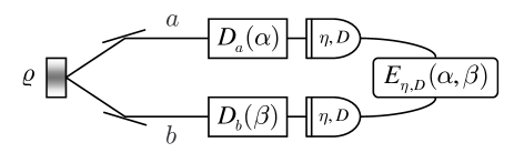
Figure 23: Scheme of the nonlocality test based on displaced on/off photodetection: the two modes $a$ and $b$ of a bipartite state $\varrho$ are locally displaced by an amount $\alpha$ and $\beta$ respectively, and then revealed through on/off photodetection. The corresponding correlation function violates Bell’s inequalities for dichotomic measurements for a suitable choice of the parameters $\alpha$ and $\beta$, depending on the kind of state under investigation. The violation holds also for non-unit quantum efficiency and non-zero dark counts.

The nonlocality test we are going to analyze is schematically depicted in Fig. 23: two modes of the de-Gaussified TWB radiation field, $a$ and $b$, described by the density matrix $\varrho$, are locally displaced by an amount $\alpha$ and $\beta$ respectively and, finally, they are revealed by on/off photodetectors, i.e., detectors which have no output when no photon is detected and a fixed output when one or more photons are detected. The action of an on/off detector is described by the following two-value positive operator-valued measure (POVM) $\{\Pi_{0,\eta,D},\Pi_{1,\eta,D}\}$ FOP:napoli:05

$${\Pi}_{0,\eta,D}=\frac{1}{1+D}\>\sum_{k=0}^{\infty}\left(1-\frac{\eta}{1+D}\right)^{k}|k\rangle\langle k|\>,$$ (100a)

$${\Pi}_{1,\eta,D}=\mathbb{I}-{\Pi}_{0,\eta,D}\>,$$ (100b)

$\eta$ being the quantum efficiency and $D$ the mean number of dark counts, i.e., of clicks with vacuum input. In writing Eq. (100) we have considered a thermal background as the origin of dark counts. An analogous expression may be written for a Poissonian background IOP:05 . For small values of the mean number $D$ of dark counts (as it generally happens at optical frequencies) the two kinds of background are indistinguishable.

Overall, taking into account the displacement, the measurement on both modes $a$ and $b$ is described by the POVM (we are assuming the same quantum efficiency and dark counts for both the photodetectors)

$${\Pi}_{hk}^{(\eta,D)}(\alpha,\beta)={\Pi}_{h}^{(\eta,D)}(\alpha)\,\otimes{\Pi}_{k}^{(\eta,D)}(\beta)\,\;,$$ (101)

where $h,k=0,1$, and ${\Pi}_{h}^{(\eta,D)}(z)\equiv D(z)\,{\Pi}_{h,\eta,D}\,D^{{\dagger}}(z)$, $D(z)=\exp\left\{za^{\dagger}-z^{*}a\right\}$ being the displacement operator and $z\in{\mathbb{C}}$ a complex parameter.

In order to analyze the nonlocality of the state $\varrho$, we introduce the following correlation function:

$$E_{\eta,D}(\alpha,\beta) =\sum_{h,k=0}^{1}(-)^{h+k}\,\left\langle{\Pi}_{hk}^{(\eta,D)}(\alpha,\beta)\right\rangle$$ (102)

$$=1+4\,{\cal I}_{\eta,D}(\alpha,\beta)-2\,\left[{\cal G}_{\eta,D}(\alpha)+{\cal Y}_{\eta,D}(\beta)\right]\>,$$

where

$${\cal I}_{\eta,D}(\alpha,\beta)=\left\langle{\Pi}_{00}^{(\eta,D)}(\alpha,\beta)\right\rangle$$ (103)

$${\cal G}_{\eta,D}(\alpha)=\left\langle{\Pi}_{0}^{(\eta,D)}(\alpha)\otimes\mathbb{I}\right\rangle$$ (104)

$${\cal Y}_{\eta,D}(\beta)=\left\langle\mathbb{I}\otimes{\Pi}_{0}^{(\eta,D)}(\beta)\right\rangle\>,$$ (105)

and where $\langle A\rangle\equiv{\rm Tr}[\varrho\,A]$ denotes ensemble average on both the modes. The so-called Bell parameter is defined by considering four different values of the complex displacement parameters as follows:

$${\cal B}_{\eta,D} =E_{\eta,D}(\alpha,\beta)+E_{\eta,D}(\alpha^{\prime},\beta)$$

$$\hskip 28.45274pt+E_{\eta,D}(\alpha,\beta^{\prime})-E_{\eta,D}(\alpha^{\prime},\beta^{\prime})$$ (106)

$$=\>\>2+4\left\{{\cal I}_{\eta,D}(\alpha,\beta)+{\cal I}_{\eta,D}(\alpha^{\prime},\beta)+{\cal I}_{\eta,D}(\alpha,\beta^{\prime})\right.$$

$$\left.\hskip 28.45274pt-{\cal I}_{\eta,D}(\alpha^{\prime},\beta^{\prime})-{\cal G}_{\eta,D}(\alpha)-{\cal Y}_{\eta,D}(\beta)\right\}\,.$$ (107)

Any local theory implies that $|{\cal B}_{\eta,D}|$ satisfies the CHSH version of the Bell inequality, i.e., $|{\cal B}_{\eta,D}|\leq 2$ $\forall\alpha,\alpha^{\prime},\beta,\beta^{\prime}$ CHSH , while quantum mechanical description of the same kind of experiments does not impose this bound.

Notice that using Eqs. (100) and (103)–(105), we obtain the following scaling properties for the functions ${\cal I}_{\eta,D}(\alpha,\beta)$, ${\cal G}_{\eta,D}(\alpha)$ and ${\cal Y}_{\eta,D}(\beta)$

$${\cal I}_{\eta,D}(\alpha,\beta)=\left(\frac{1}{1+D}\right)^{2}\,{\cal I}_{\eta/(1+D)}(\alpha,\beta)$$ (108)

$${\cal G}_{\eta,D}(\alpha)=\frac{1}{1+D}\,{\cal G}_{\eta/(1+D)}(\alpha)$$ (109)

$${\cal Y}_{\eta,D}(\beta)=\frac{1}{1+D}\,{\cal Y}_{\eta/(1+D)}(\beta)$$ (110)

where ${\cal I}_{\eta}={\cal I}_{\eta,0}$, ${\cal G}_{\eta}={\cal G}_{\eta,0}$, and ${\cal Y}_{\eta}={\cal Y}_{\eta,0}$. Therefore, it will be enough to study the Bell parameter for $D=0$, namely ${\cal B}_{\eta}={\cal B}_{\eta,0}$, and then we can use Eqs. (108)–(110) to take into account the effects of non negligible dark counts. From now on we will assume $D=0$ and suppress the explicit dependence on $D$. Notice that using expression (107) for the Bell parameter the CHSH inequality $|{\cal B}_{\eta,D}|\leq 2$ can be rewritten as

$$-1< \>\>{\cal I}_{\eta,D}(\alpha,\beta)+{\cal I}_{\eta,D}(\alpha^{\prime},\beta)+{\cal I}_{\eta,D}(\alpha,\beta^{\prime})$$

$$-{\cal I}_{\eta,D}(\alpha^{\prime},\beta^{\prime})-{\cal G}_{\eta,D}(\alpha)-{\cal Y}_{\eta,D}(\beta)<0\;,$$ (111)

which represents the CH version of the Bell inequality for our system CH .

In order to simplify the calculations, throughout this Section we will use the Wigner formalism. The Wigner functions associated with the elements of the POVM (100) for $D=0$ are given by IOP:05

$$W[\Pi_{0,\eta}](z) =\frac{\Delta_{\eta}}{\pi\eta}\,\exp\left\{-\Delta_{\eta}\,|z|^{2}\right\}\,,$$ (112)

$$W[\Pi_{1,\eta}](z) =W[\mathbb{I}](z)-W[\Pi_{0,\eta}](z)\,,$$ (113)

with $\Delta_{\eta}=2\eta/(2-\eta)$, and $W[\mathbb{I}](z)=\pi^{-1}$. Then, noticing that for any operator $O$ one has

$$W[D(\alpha)\,O\,D^{{\dagger}}(\alpha)](z)=W[O](z-\alpha)\,,$$ (114)

it follows that $W[D(\alpha)\,{\Pi}_{0,\eta}\,D^{{\dagger}}(\alpha)](z)$ is given by

$$W[D(\alpha)\,{\Pi}_{0,\eta}\,D^{{\dagger}}(\alpha)](z)=W[\Pi_{0,\eta}](z-\alpha)\,,$$ (115)

and therefore

$$W[\Pi_{00}^{(\eta,0)}(\alpha,\beta)](z,w) =W[\Pi_{0,\eta}](z-\alpha)\,W[\Pi_{0,\eta}](w-\beta)$$ (116)

$$W[\Pi_{0,\eta}(\alpha)\otimes\mathbb{I}](z,w) =W[\Pi_{0,\eta}](z-\alpha)\>\pi^{-1}$$ (117)

$$W[\mathbb{I}\otimes\Pi_{0,\eta}(\beta)](z,w) =\pi^{-1}\>W[\Pi_{0,\eta}](w-\beta)\;.$$ (118)

Finally, thanks to the trace rule expressed in the phase space of two modes, i.e.,

$${\rm Tr}[O_{1}\,O_{2}]=\pi^{2}\int_{\mathbb{C}^{2}}\!d^{2}z\>d^{2}w\,W[O_{1}](z,w)\,W[O_{2}](z,w)\,,$$ (119)

one can evaluate the functions ${\cal I}_{\eta}(\alpha,\beta)$, ${\cal G}_{\eta}(\alpha)$, and ${\cal Y}_{\eta}(\beta)$, and in turn the Bell parameter ${\cal B}_{\eta}$ in Eq. (107), as a sum of Gaussian integrals in the complex plane.

Let us now consider the TWB (25). Since the Wigner functions of the TWB and of the POVM (101) are Gaussian, it is quite simple to evaluate ${\cal I}_{\eta}(\alpha,\beta)$, ${\cal G}_{\eta}(\alpha)$, and ${\cal Y}_{\eta}(\beta)$ of the correlation function (102) and, then, ${\cal B}_{\eta}$; we have

$${\cal I}_{\eta}(\alpha,\beta)=\frac{{\cal M}_{\eta}(r)}{\eta^{2}\sqrt{{\rm Det}[\boldsymbol{\sigma}_{0}]}}\,$$

$$\hskip 28.45274pt\times\exp\big{\{}-\widetilde{F}_{\eta}\,(|\alpha|^{2}+|\beta|^{2})+\widetilde{H}_{\eta}\,(\alpha\beta+\alpha^{*}\beta^{*})\big{\}}$$ (120)

$${\cal G}_{\eta}(\alpha)={\cal Y}_{\eta}(\alpha)=\frac{\left(2\sqrt{{\rm Det}[\boldsymbol{\sigma}_{0}]}\right)^{-1}\Delta_{\eta}}{[2(\widetilde{A}_{0}^{2}-\widetilde{B}_{0}^{2})+\widetilde{A}_{0}\Delta_{\eta}]}$$

$$\hskip 28.45274pt\times\exp\left\{-\frac{2\Delta_{\eta}}{2(\widetilde{A}_{0}^{2}-\widetilde{B}_{0}^{2})+\widetilde{A}_{0}\Delta_{\eta}}\,|\alpha|^{2}\right\}$$ (121)

with

$$\widetilde{F}_{\eta}\equiv\widetilde{F}_{\eta}(r)=\Delta_{\eta}-(2\widetilde{A}_{0}+\Delta_{\eta})\,{\cal M}_{\eta}(r)$$ (122)

$$\widetilde{H}_{\eta}\equiv\widetilde{H}_{\eta}(r)=2\widetilde{B}_{0}{\cal M}_{\eta}(r)$$ (123)

$${\cal M}_{\eta}(r)=\frac{\Delta_{\eta}^{2}}{4(\widetilde{A}_{0}^{2}-\widetilde{B}_{0}^{2})+4\widetilde{A}_{0}\Delta_{\eta}+\Delta_{\eta}^{2}}\,,$$ (124)

In order to study Eq. (107), we consider the parametrization $\alpha=-\beta={\cal J}$ and $\alpha^{\prime}=-\beta^{\prime}=-\sqrt{11}{\cal J}$ (more details are given in IOP:05 ). The parametrization was chosen after a semi-analytical analysis and maximizes the violation of the Bell’s inequality (for $\eta=1$). In Fig. 24 we plot ${\cal B}_{\eta}$ for $\eta=1$: as one can see the inequality $|{\cal B}_{\eta}|\leq 2$ is violated for a wide range of parameters, and the maximum violation (${\cal B}_{\eta}=2.45$) is achieved when ${\cal J}=0.16$ and $r=0.74$. The effect of non-unit efficiency in the detection stage is to reduce the the violation; this is shown in Fig. 25, where we plot ${\cal B}_{\eta}$ as a function of ${\cal J}$ with $r=0.74$ for different values of the quantum efficiency. Note that though the violation in the ideal case, i.e., $\eta=1$, is smaller than for the Bell states, the TWBs are more robust when one takes into account non-unit quantum efficiency.

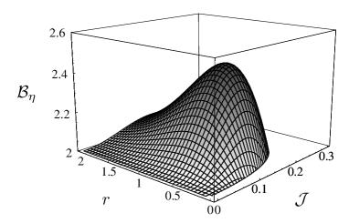
Figure 24: Plot of ${\cal B}_{\eta}$ for a TWB as a function of ${\cal J}$ and the TWB squeezing parameter $r$ in the case of ideal (i.e., $\eta=1$) on/off photodetection. The maximum violation is ${\cal B}_{\eta}=2.45$, which is obtained when ${\cal J}=0.16$ and $r=0.74$.

Figure 25: Plot of ${\cal B}_{\eta}$ for a TWB as a function of ${\cal J}$ with $r=0.74$ for different values of $\eta$: from top to bottom $\eta=1.0$, $0.9$, $0.85$, and $0.80$.

In the case of the state (54), the correlation function (102) reads (for the sake of simplicity we do not write explicitly the dependence on $r$, $T$ and $\varepsilon$)

$$E_{\eta}(\alpha,\beta)=1+\frac{1}{p_{11}(r,T,\varepsilon)}\sum_{k=1}^{4}{\cal C}_{k}\,\big{\{}4\,{\cal I}^{(k)}_{\eta}(\alpha,\beta)\\ -2\big{[}{\cal G}^{(k)}_{\eta}(\alpha)+{\cal Y}^{(k)}_{\eta}(\beta)\big{]}\big{\}}\,,$$ (125)

where

$${\cal I}^{(k)}_{\eta}(\alpha,\beta)=\frac{{\cal M}_{\eta}^{(k)}(r,T,\varepsilon)}{\eta^{2}}\,$$

$$\times\exp\big{\{}-\widetilde{G}_{\eta}^{(k)}\,|\alpha|^{2}-\widetilde{F}_{\eta}^{(k)}\,|\beta|^{2}+\widetilde{H}_{\eta}^{(k)}\,(\alpha\beta+\alpha^{*}\beta^{*})\big{\}}\,,$$ (126)

$${\cal G}^{(k)}_{\eta}(\alpha)=\frac{\Delta_{\eta}}{[G_{k}\,(F_{k}+\Delta_{\eta})-H_{k}^{2}]\,\eta}$$

$$\hskip 28.45274pt\times\exp\left\{-\frac{(F_{k}G_{k}-H_{k}^{2})\,\Delta_{\eta}}{G_{k}\,(F_{k}+\Delta_{\eta})-H_{k}^{2}}\,|\alpha|^{2}\right\}\,,$$ (127)

$${\cal Y}^{(k)}_{\eta}(\beta)=\frac{\Delta_{\eta}}{[F_{k}\,(G_{k}+\Delta_{\eta})-H_{k}^{2}]\,\eta}$$

$$\hskip 28.45274pt\times\exp\left\{-\frac{(F_{k}G_{k}-H_{k}^{2})\,\Delta_{\eta}}{F_{k}\,(G_{k}+\Delta_{\eta})-H_{k}^{2}}\,|\beta|^{2}\right\}\,.$$ (128)

with $\widetilde{F}_{\eta}^{(k)}\equiv\widetilde{F}_{\eta}^{(k)}(r,T,\varepsilon)$, $\widetilde{G}_{\eta}^{(k)}\equiv\widetilde{G}_{\eta}^{(k)}(r,T,\varepsilon)$, and $\widetilde{H}_{\eta}^{(k)}\equiv\widetilde{H}_{\eta}^{(k)}(r,T,\varepsilon)$ given by

$$\widetilde{F}_{\eta}^{(k)}=\Delta_{\eta}-(F_{k}+\Delta_{\eta})\,{\cal M}_{\eta}^{(k)}(r,T,\varepsilon)\,,$$ (129)

$$\widetilde{G}_{\eta}^{(k)}=\Delta_{\eta}-(G_{k}+\Delta_{\eta})\,{\cal M}_{\eta}^{(k)}(r,T,\varepsilon)\,,$$ (130)

$$\widetilde{H}_{\eta}^{(k)}=H_{k}\,{\cal M}_{\eta}^{(k)}(r,T,\varepsilon)\,,$$ (131)

$${\cal M}_{\eta}^{(k)}(r,T,\varepsilon)=\frac{\Delta_{\eta}^{2}}{(F_{k}+\Delta_{\eta})(G_{k}+\Delta_{\eta})-H_{k}^{2}}\,,$$ (132)

where $F_{k}=b-f_{h}$, $G_{k}=b-g_{h}$, and $H_{k}=2\widetilde{B}_{0}T-h_{k}$ and all the involved quantities are the same as in Eq. (54).

In order to study Eq. (107), we consider the parametrization $\alpha=-\beta={\cal J}$ and $\alpha^{\prime}=-\beta^{\prime}=-\sqrt{11}{\cal J}$. This parametrization was chosen after a semi-analytical analysis and maximizes the violation of the Bell’s inequality (for $\eta=1$) IOP:05 . The results are showed in Figs. 26 and 27 for $\eta=1$ and $\varepsilon=1$: we can see that the IPS enhances the violation of the inequality $|{\cal B}_{\eta}|\leq 2$ for small values of $r$ (see also Refs. OP:PSnoise ; ips:PRA:67 ; ips:PRA:70 ). Moreover, as one may expect, the maximum of violation is achieved as $T\to 1$, whereas decreasing the effective transmission of the IPS process, one has that the inequality becomes satisfied for all the values of $r$, as we can see in Fig. 27 for $T=0.6$.

In Fig. 28 we plot ${\cal B}_{\eta}$ for the IPS with $T=0.9999$, $\varepsilon=1$ and different $\eta$. As for the TWB, we can have violation of the Bell’s inequality also for detection efficiencies near to $80\%$. As for the Bell states and the TWB, a $\eta$- and $r$-dependent choice of the parameters in Eq. (107) can improve this result.

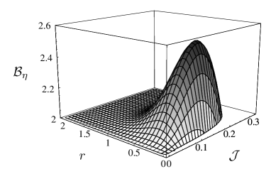
Figure 26: Plot of ${\cal B}_{\eta}$ for the IPS state with $T=0.9999$ and $\varepsilon=1$ as a function of ${\cal J}$ and the TWB squeezing parameter $r$ in the case of ideal (i.e., $\eta=1$) on/off photodetection. The maximum violation is ${\cal B}_{\eta}=2.53$, which is obtained when ${\cal J}=0.16$ and $r=0.39$.

Figure 27: Plot of ${\cal B}_{\eta}$ for the IPS state as a function of ${\cal J}$ with $r=0.39$ for different values of $T$ and $\varepsilon=1$ in the ideal case (i.e., $\eta=1$): from top to bottom $T=0.9999$, $0.90$, $0.80$, $0.70$, and $0.60$.

Figure 28: Plot of ${\cal B}_{\eta}$ for the IPS state as a function of ${\cal J}$ with $r=0.39$, $T=0.9999$, $\varepsilon=1$, and for different values of $\eta$: from top to bottom $\eta=1.0$, $0.9$, $0.85$, and $0.8$.

The effect on a non-unit $\varepsilon$ is studied in Fig. 29, where we plot ${\cal B}_{\eta}$ as a function of $T$ and $\varepsilon$ and fixed values of the other involved parameters. We can see that the main effect on the Bell parameter is due to the transmissivity $T$.

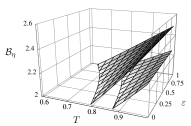
Figure 29: Plot of ${\cal B}_{\eta}$ for the IPS state as a function $T$ and $\varepsilon$ with ${\cal J}=0.16$, $r=0.39$, and, from top to bottom, $\eta=0.99$, and $0.90$. The main effect on ${\cal B}_{\eta}$ is due to the transmissivity $T$.

Finally, the effect of dissipation and thermal noise affecting the propagation of the TWB before the IPS process is shown in Fig. 30.

Figure 30: Plot of ${\cal B}_{\eta}$ for the IPS state as a function of ${\cal J}$ with $r=0.39$, $T=0.99$, $\varepsilon=1$, $\eta=0.9$, and $\Gamma t=0.1$ for different values of $N$: from top to bottom (solid lines) $N=0$, $0.01$, and $0.02$. The dashed line is ${\cal B}_{\eta}$ with $\Gamma t=N=0$.

X Conclusions

We have analyzed in details a photon subtraction scheme to de-Gaussify states of radiation and, in particular, to enhance nonlocal properties of twin-beams. The scheme is based on conditional inconclusive subtraction of photons (IPS), which may be achieved by means of linear optical components and avalanche on/off photodetectors. The IPS process can be implemented with current technology and, indeed, application to single-mode state has been recently realized with high conditional probability weng:PRL:04 .

We found that IPS process improves fidelity of coherent state teleportation and show, by using several different nonlocality tests, that it also enhances nonlocal correlations. IPS may be profitably used also on nonmaximmally mixed entangled states, as the ones coming from the evolution of TWB in a noisy channel. In addition, the effectiveness of the process is not dramatically influenced either by the transmissivity of the beam-splitter used to subtract photons, not by the quantum efficiency of the detectors used to reveal them.

We conclude that IPS on TWB is a robust and realistic scheme to improve quantum information processing with CV radiation states.

XI Acknowledgments

This work has been supported by MIUR through the project PRIN-2005024254-002.

References

(1) S. Braunstein, and P. van Loock, Rev.
Mod. Phys. 77, 513 (2005).
(2) A. Ferraro, S. Olivares, and M. G. A. Paris,
“Gaussian States in Quantum Information”, Napoli Series on
Physics and Astrophysics (Bibliopolis, Napoli, 2005); e-print,
quant-ph/0503237.
(3)Quantum Interferometry III, Special issue of
Fort. Phys. 48 (2000), F. De Martini, G. Denardo, and L. Hardy Eds.;
Quantum Interferometry IV, Special issue of
Fort. Phys. 51 (2003), F. De Martini Ed.
(4)Quantum Communication, Computing and Measurement II,
P. Kumar, G. M. D’Ariano, and O. Hirota Eds., (Kluver Academic,
Dordrecht, 2000); Quantum Communication, Computing, and Measurements
III, P. Tombesi, and O. Hirota Eds., (Kluwer/Plenum, Dordrecht, 2001).
(5) A. Furusawa, et al., Science 282, 706 (1998);
S. L. Braunstein, and H. J. Kimble, Phys. Rev. Lett. 80, 869 (1998).
(6) S. L. Braunstein, and H. J. Kimble, Phys. Rev. A
61, 042302 (2000); J. Jing et al., Phys. Rev. Lett. 90,
167903 (2003).
(7) H. Yonezawa, T. Aoki and A. Furusawa, Nature 431, 430
(2004).
(8) T. Opatrný, G. Kurizki, and D.-G. Welsch, Phys. Rev. A
61, 032302 (2000).
(9) P. T. Cochrane, T. C. Ralph, and G. J. Milburn, Phys. Rev. A
65, 062306 (2002).
(10) S. Olivares, M. G. A. Paris, and R. Bonifacio, Phys.
Rev. A 67, 032314 (2003).
(11) J. Wenger, R. Tualle-Brouri, and P. Grangier, Phys.
Rev. Lett. 92, 153601 (2004).
(12) M. S. Kim, E. Park, P. L. Knight, and H. Jeong, Phys. Rev.
A 71, 013801 (2005).
(13) S. Olivares, and M. G. A. Paris, J. Opt. B:
Quantum and Semiclass. Opt. 7, S616 (2005).
(14) S. Olivares, and M. G. A. Paris, Phys. Rev. A 70, 032112 (2004).
(15) S. Olivares, and M. G. A. Paris, J. Opt. B:
Quantum and Semiclass. Opt. 7, S392 (2005) .
(16) H. Nha, and H. J. Carmichael, Phys. Rev. Lett. 93,
020401 (2004).
(17) R. García-Patrón, et al., Phys.
Rev. Lett. 93, 130409 (2004); R. García-Patrón, J. Fiurášek, and N. J Cerf, Phys. Rev. A 71, 022105 (2005).
(18) S. Daffer, and P. L. Knight, Phys. Rev. A 72, 032509
(2005).
(19) C. Invernizzi, S. Olivares, M. G. A. Paris, and
K. Banszek, Phys. Rev. A 72 042105 (2005).
(20) M. Dakna et al, Phys. Rev. A 55, 3184 (1997).
(21) F. Zappa, A. L. Lacaita, S. D. Cova, and
P. Lovati, Opt. Eng. 35, 938 (1996); D.‘Achilles, C. Silberhorn,
C. liwa, K.‘Banaszek, and I. A. Walmsley,
Opt. Lett. 28, 2387 (2003).
(22) G. Di Giuseppe, A. V. Sergienko, B. E. A. Saleh, and
M. C. Teich in Quantum Information and Computation, E. Donkor,
A. R. Pirich, and H. E. Brandt Eds., Proceedings of the SPIE 5105, 39 (2003).
(23) A. R. Rossi, S. Olivares, and M. G. A. Paris, Phys. Rev. A
70, 055801 (2004).
(24) M. Bondani, et. al., Phys. Rev. Lett. 95, 063602
(2005).
(25) D. Walls, and G. Milburn, Quantum Optics
(Springer, Berlin, 1994).
(26) S. Olivares, and M. G. A. Paris, J. Opt. B: Quantum
Semiclass. Opt. 6, 69 (2004).
(27) A. Serafini, F. Illuminati, M. G. A. Paris, and
S. De Siena, Phys. Rev. A 69, 023318 (2004).
(28) M. G. A. Paris, M. Cola, and R. Bonifacio, Phys. Rev. A
67, 042104 (2003).
(29) J. F. Clauser, M. A. Horne, A. Shimony, and R. A. Holt,
Phys. Rev. Lett. 23, 880 (1969).
(30) K. Banaszek, and K. Wódkiewicz, Phys. Rev. A 58,
4345 (1998).
(31) S. Olivares, and M. G. A. Paris, Phys. Rev. A 70,
032112 (2004).
(32) H. Jeong et al., Phys. Rev. A 67, 012106 (2003).
(33) A. Gilchrist, P. Deuar, and M. D. Reid, Phys. Rev. Lett. 80, 3169 (1998); A. Gilchrist, P. Deuar, and M. D. Reid, Phys. Rev. A 60,
4259 (1999).
(34) W. J. Munro, Phys. Rev. A 59, 4197 (1999).
(35) R. Filip, and L. Mista, Phys. Rev. A 66,
044309 (2002).
(36) Z.-B. Chen, J.-W. Pan, G. Hou, and Y.-D. Zhang, Phys.
Rev. Lett. 88, 040406 (2002).
(37) G. Gour et al., Phys. Lett. A 324, 415 (2003);
M. Revzen, et al., Phys. Rev. A 71, 022103 (2005).
(38)A. Ferraro, and M. G. A. Paris, J. Opt. B:
Quantum Semiclass. Opt. 7, 174 (2005).
(39) J. F. Clauser, and M. A. Horne, Phys. Rev. D 10, 526
(1974).