Quantum Nondemolition Measurement of Discrete Fock States of a Nanomechanical Resonator

Abstract

We study theoretically a radio frequency superconducting interference device integrated with a nanomechanical resonator and an LC resonator. By applying adiabatic and rotating wave approximations, we obtain an effective Hamiltonian that governs the dynamics of the mechanical and LC resonators. Nonlinear terms in this Hamiltonian can be exploited for performing a quantum nondemolition measurement of Fock states of the nanomechanical resonator. We address the feasibility of experimental implementation and show that the nonlinear coupling can be made sufficiently strong to allow the detection of discrete mechanical Fock states.

Anharmonicity may introduce coupling between different modes of a resonator. In a seminal paper Sanders and Milburn (1989), Sanders and Milburn found that inter-mode coupling could in principle enable quantum non-demolition (QND) detection Braginsky and Khalili (1995); Caves et al. (1980) of discrete Fock states of a signal mode by intensively driving another nonlinearly coupled detector (or pump) mode, and monitoring the response near the pump frequency. Such a measurement scheme is characterized by a measurement time $\tau_{m}$, defined as the time needed to distinguish between initial states of the signal mode having different Fock numbers. Fock number detection can be realized if $\tau_{m}$ can be made shorter than the lifetime of a Fock state of the signal mode.

The prospects of employing this technique for QND measurement of a single phonon in a mesoscopic mechanical resonator was recently studied theoretically in Ref. Santamore et al. (2004a). In practice, however, anharmonic couplings between different modes of a mechanical resonator are typically far too weak to allow single-phonon detection when the detector mode is taken to have a linear response. On the other hand, a significant enhancement can be achieved by driving the detector mode into the nonlinear regime and exploiting critical slowing down by operating close to the edge of the region where the response exhibits bistability Santamore et al. (2004b); Buks and Yurke (2006a).

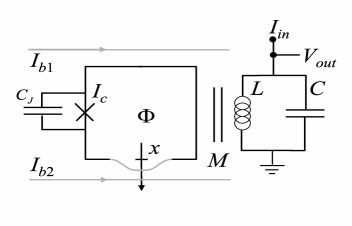
Figure 1: The device consists of an RF SQUID integrated with a nanomechanical and an LC resonators. The external flux is applied by using 2 bias current lines carrying dc currents $I_{b1}$ and $I_{b2}$ respectively. One of the current line lies very close to the vibrating beam, allowing thus a relatively high value of the magnetic field $B$ at the location of the beam. On the other hand, the Josephson junction is located symmetrically in such a way that the magnetic field at its location vanishes when $I_{b1}=I_{b2}$. This configuration allows applying the needed external flux to the loop $\Phi_{e}=\Phi_{0}/2$ without significantly degrading the critical current of the junction provided that the area of the junction is kept much smaller than the area of the loop.

To achieve single phonon sensitivity, it is highly desirable to increase the anharmonic coupling between the signal mode and the detector mode. Here we propose a novel configuration in which a fundamental mode of a doubly clamped beam, serving as the mechanical signal mode, is indirectly coupled to an LC resonator serving as the detector. The anharmonic coupling is achieved by coupling both the mechanical mode and the LC resonator directly to a radio frequency superconducting interference device (RF SQUID) Buks and Blencowe (2006). We show that the RF SQUID degree of freedom can be eliminated from the equations of motion by employing an adiabatic approximation. Moreover, employing the rotating wave approximation (RWA) leads to further simplification of the equations of motion of the system. We find that the effective anharmonic coupling constant between the mechanical mode and the LC resonator in this configuration can be made sufficiently large to allow single phonon detection under appropriate conditions.

Alternative approaches for performing QND measurement of the energy of a nanomechanical resonator were proposed recently in Refs. Jacobs et al. (2007b, a). Similar systems consisting of a SQUID integrated with a nanomechanical resonator have been recently studied theoretically Blencowe and Buks (2007); Buks et al. (2007). Zhou and Mizel have shown that nonlinear coupling between a DC SQUID and a mechanical resonator can be employed for producing squeezed states of the mechanical resonator Zhou and Mizel (2006). More recently, Xue et al. have shown that a flux qubit integrated with a nanomechanical resonator can form a cavity quantum electrodynamics system in the strong coupling region Xue et al. (2007).

The device, which is seen in Fig. 1, consists of an RF SQUID inductively coupled to an LC resonator. A section of the RF SQUID loop is freely suspended and allowed to oscillate mechanically. We assume the case where the fundamental mechanical mode vibrates in the plane of the loop and denote the amplitude of this flexural mode as $x$. Let $m$ be the effective mass of the fundamental mode, and $\omega_{m}$ its angular resonance frequency. A magnetic field is applied perpendicularly to the plane of the loop. Let $\Phi_{e}$ be the externally applied flux for the case $x=0$, and let $B$ denote the component of the magnetic field normal to the plane of the loop at the location of the doubly clamped beam (it is assumed that $B$ is constant in the region where the beam oscillates). A Josephson junction (JJ) having a critical current $I_{c}$ and capacitance $C_{J}$ is integrated into the loop. The RF SQUID is inductively coupled to a resonator comprising an inductor $L$ and a capacitor $C$ in parallel. The mutual inductance between the RF SQUID and the resonator is $M$. Detection is performed by injecting a monochromatic input current $I_{in}$ into the LC resonator and measuring the output voltage $V_{out}$ (see Fig. 1).

The total magnetic flux $\Phi$ threading the loop is given by $\Phi=\Phi_{e}+Blx+\Phi_{i}$, where $l$ is an effective length of the beam. The term $\Phi_{i}=I_{s}\Lambda+MI_{L}$ represents the flux generated by both the circulating current in the RF SQUID $I_{s}$ and by the current in the inductor of the LC resonator $I_{L},$where $\Lambda$ is the self inductance of the loop. Similarly, the magnetic flux in the inductor of the LC resonator is given by $\varphi=I_{L}L+MI_{s}$.

The gauge invariant phase across the Josephson junction is given by $\theta=2\pi n-2\pi\Phi/\Phi_{0}$, where $n$ is integer and $\Phi_{0}=h/2e$ is the flux quantum.

The Lagrangian of the closed system is expressed as a function of $x$, $\varphi$ and $\Phi$ and their time derivatives (denoted by overdot)

$$\mathcal{L}=\frac{m\dot{x}^{2}}{2}+\frac{C\dot{\varphi}^{2}}{2}+\frac{C_{J}\dot{\Phi}^{2}}{2}-U_{0}-U_{1}\ ,$$ (1)

where the potential terms are given by

$$U_{0} =\frac{m\omega_{m}^{2}x^{2}}{2}+\frac{C\omega_{e}^{2}\varphi^{2}}{2}-I_{in}\varphi\ ,$$ (2a)

$$U_{1} =\frac{\left(\Phi-\Phi_{e}-Blx-\frac{M\varphi}{L}\right)^{2}}{2\Lambda\left(1-K^{2}\right)}-\frac{\Phi_{0}I_{c}\cos\frac{2\pi\Phi}{\Phi_{0}}}{2\pi}\ ,$$ (2b)

and where $$\omega_{e}=1/\sqrt{LC} K=M/\sqrt{\Lambda L}$$ and .

The Euler - Lagrange equations can be written as

$$m\ddot{x}+m\omega_{m}^{2}x-BlI_{s} =0\ ,$$ (3a)

$$C\ddot{\varphi}+I_{L}-I_{in} =0\ ,$$ (3b)

$$C_{J}\ddot{\Phi}+I_{s}+I_{c}\sin\frac{2\pi\Phi}{\Phi_{0}} =0\ .$$ (3c)

The interpretation of these equations is straightforward. Eq. (3a) is Newton’s 2nd law for the mechanical resonator, where the force is composed of the restoring elastic force $$-m\omega_{m}^{2}x BlI_{s} I_{in} I_{L} C\ddot{\varphi} I_{s} I_{c}\sin\theta C_{J}\dot{V}_{J} V_{J} V_{J}=\left(\Phi_{0}/2\pi\right)\dot{\theta}$$ and the Lorentz force acting on the movable beam. Eq. (3b) states that the injected current into the LC resonator equals the sum of the current in the inductor and the one in the capacitor . Similarly, Eq. (3c) states that the circulating current equals the sum of the current through the JJ and the current through the capacitor, where the voltage across the JJ is given by the second Josephson equation .

The variables canonically conjugate to $x$, $\varphi$ and $\Phi$ are given by $p=\partial\mathcal{L}/\partial\dot{x}$, $q=\partial\mathcal{L}/\partial\dot{\varphi}$ and $Q=\partial\mathcal{L}/\partial\dot{\Phi}$ respectively. The Hamiltonian is given by

$$\mathcal{H}=\mathcal{H}_{0}+\mathcal{H}_{1}\ ,$$ (4)

where

$$\mathcal{H}_{0} =\frac{p^{2}}{2m}+\frac{q^{2}}{2C}+U_{0}\ ,$$ (5a)

$$\mathcal{H}_{1} =\frac{Q^{2}}{2C_{J}}+U_{1}\ .$$ (5b)

Quantization is achieved by regarding the variables $$x, p, \varphi, q, \Phi Q$$ and as Hermitian operators satisfying canonical commutation relations.

As a basis for expanding the general solution we use the eigenvectors of the following Schrödinger equation

$$\mathcal{H}_{1}\left|n\left(x,\varphi\right)\right\rangle=\varepsilon_{n}\left(x,\varphi\right)\left|n\left(x,\varphi\right)\right\rangle\ ,$$ (6)

where $x$ and $\varphi$ are treated here as parameters (rather than degrees of freedom). The local eigen-vectors are assumed to be orthonormal $\left\langle m\left(x,\varphi\right)|n\left(x,\varphi\right)\right\rangle=\delta_{nm}$.

The eigenenergies $\varepsilon_{n}\left(x,\varphi\right)$ and the associated wavefunctions $\vartheta_{n}$ are found by solving the following Schrödinger equation

$$\left(-\beta_{C}\frac{\partial^{2}}{\partial\phi^{2}}+u\right)\vartheta_{n}=\frac{\varepsilon_{n}}{E_{0}}\vartheta_{n}\ .$$ (7)

where

$$u =\frac{\left(\phi-\phi_{0}\right)^{2}}{1-K^{2}}+2\beta_{L}\cos\phi\ ,$$ (8)

$$\phi =\frac{2\pi}{\Phi_{0}}\left(\Phi-\frac{\Phi_{0}}{2}\right)\ ,$$ (9)

$$\phi_{0} =\frac{2\pi}{\Phi_{0}}\left(\Phi_{e}-\frac{\Phi_{0}}{2}+Blx+\frac{M\varphi}{L}\right)\ ,$$ (10)

$\beta_{L}=2\pi\Lambda I_{c}/\Phi_{0}$, $\beta_{C}=2e^{2}/C_{J}E_{0}$ and $E_{0}=\Phi_{0}^{2}/8\pi^{2}\Lambda$.

The total wave function is expanded as

$$\psi=\sum\nolimits_{n}\xi_{n}\left(x,\varphi,t\right)\left|n\right\rangle\ .$$

In the adiabatic approximation Moody et al. (1989) the time evolution of the coefficients $\xi_{n}$ is governed by the following set of decoupled equations of motion

$$\left[\mathcal{H}_{0}+\varepsilon_{n}\left(x,\varphi\right)\right]\xi_{n}=i\hbar\dot{\xi}_{n}\ .$$ (11)

Note that in the present case the geometrical vector potential Moody et al. (1989) vanishes. The validity of the adiabatic approximation will be discussed below.

In what follows we focus on the case where $\left|\phi_{0}\right|\ll 1$ and $\beta_{L}\left(1-K^{2}\right)>1$. In this case the adiabatic potential $u\left(\phi\right)$ given by Eq. (8) contains two wells separated by a barrier near $\phi=0$. At low temperatures only the two lowest energy levels contribute. In this limit the local Hamiltonian $\mathcal{H}_{1}$ can be expressed in the basis of the states $\left|\curvearrowleft\right\rangle$ and $\left|\curvearrowright\right\rangle$, representing localized states in the left and right well respectively having opposite circulating currents. In this basis, $\mathcal{H}_{1}$ is represented by the $2\times 2$ matrix

$$\mathcal{H}_{1}\dot{=}\left(\begin{array}[c]{cc}\eta\phi_{0}&\Delta\\ \Delta&-\eta\phi_{0}\end{array}\right)\ .$$ (12)

The real parameters $\eta$ and $\Delta$ can be determined by solving numerically the Schrödinger equation (7). The eigenenergies are given by

$$\varepsilon_{\pm}=\pm\sqrt{\eta^{2}\phi_{0}^{2}+\Delta^{2}}\ .$$ (13)

It is convenient to introduce the annihilation operators

$$A_{m} =\frac{e^{i\omega_{m}t}}{\sqrt{2\hbar}}\left(\sqrt{m\omega_{m}}x+\frac{i}{\sqrt{m\omega_{m}}}p\right)\ ,$$ (14)

$$A_{e} =\frac{e^{i\omega_{e}t}}{\sqrt{2\hbar}}\left(\sqrt{C\omega_{e}}\varphi+\frac{i}{\sqrt{C\omega_{e}}}q\right)\ ,$$ (15)

and the corresponding number operators $N_{m}=A_{m}^{{\dagger}}A_{m}$ and $N_{e}=A_{e}^{{\dagger}}A_{e}$. Consider the case where $\Phi_{e}=\Phi_{0}/2$, and assume that adiabaticity holds and the RF SQUID remains in its lowest energy state. The energy of this state $\varepsilon_{-}\left(x,\varphi\right)$ can be expressed in terms of the annihilation operators $A_{m}$, $A_{e}$ and their Hermitian conjugates. The resulting expression generally contains terms oscillating at frequencies $\omega_{k,l}=k\omega_{m}+l\omega_{e}$, where $k$ and $l$ are integers. In the RWA such terms are neglected unless $\omega_{k,l}=0$ or $\omega_{k,l}$ is close to the frequency of the externally injected bias current $I_{in}$, since otherwise the effect on the dynamics on a time scale much longer than a typical oscillation period is negligibly small. Keeping terms up to fourth order in $\phi_{0}$ the eigenenergy $\varepsilon_{-}$ in the RWA can be expressed as

$$\varepsilon_{\mathrm{RWA}}\left(x,\varphi\right) =\hbar(\Omega_{0}+\Omega_{2,0}N_{m}+\Omega_{0,2}N_{e}$$

$$+\Omega_{4,0}N_{m}^{2}+\Omega_{0,4}N_{e}^{2}+\Omega_{2,2}N_{m}N_{e})\ .$$

The constant term $\hbar\Omega_{0}$ can be disregarded, since it only gives rise to a constant phase factor. Moreover, the linear terms $\hbar\Omega_{2,0}N_{m}$ and $\hbar\Omega_{0,2}N_{e}$ only give rise to a small renormalization of the resonance frequencies $\omega_{m}$ and $\omega_{e}$ respectively. In addition, since no external drive is applied directly to the mechanical oscillator, the expectation value $\left\langle N_{m}\right\rangle$ is expected to be relatively small and consequently the term proportional to $N_{m}^{2}$ can be neglected. Thus, in the RWA the Hamiltonian $\mathcal{H}_{0}+\varepsilon_{-}$, which governs the dynamics of the mechanical and LC resonators, is given by

$$\mathcal{H}_{\mathrm{RWA}} =\hbar\omega_{m}N_{m}+\hbar\omega_{e}N_{e}$$

$$-I_{in}\sqrt{\frac{\hbar}{2C\omega_{e}}}\left(e^{-i\omega_{e}t}A_{e}+e^{i\omega_{e}t}A_{e}^{{\dagger}}\right)$$

$$+\hbar\Omega_{0,4}N_{e}^{2}+\hbar\Omega_{2,2}N_{m}N_{e}\ ,$$

where

$$\Omega_{0,4}=\frac{3\Delta}{4\hbar}\left(\frac{\eta}{\Delta}\frac{2\pi M}{\Phi_{0}L}\sqrt{\frac{\hbar}{2C\omega_{e}}}\right)^{4}\ ,$$ (18)

$$\Omega_{2,2}=\frac{3\Delta}{\hbar}\left(\frac{\eta}{\Delta}\frac{2\pi Bl}{\Phi_{0}}\sqrt{\frac{\hbar}{2m\omega_{m}}}\right)^{2}\left(\frac{\eta}{\Delta}\frac{2\pi M}{\Phi_{0}L}\sqrt{\frac{\hbar}{2C\omega_{e}}}\right)^{2}\ .$$ (19)

All subsequent analysis is based on Refs. Sanders and Milburn (1989); Santamore et al. (2004a, b); Buks and Yurke (2006a), which consider how nonlinear terms of the kind appearing in the Hamiltonian $\mathcal{H}_{\mathrm{RWA}}$ can be utilized for QND detection of discrete Fock states. A single phonon added to the mechanical resonator results in a shift in the effective resonance frequency of the LC resonator. Consider first the case $\Omega_{0,4}=0$, where the response of the LC resonator is linear, and thus this frequency shift is given by $\Omega_{2,2}$. The effective resonance frequency can be continuously monitored by employing an homodyne detection scheme, in which $V_{out}$ is mixed with a local oscillator at the same frequency as the frequency of the driving current $I_{in}$. The measurement time $\tau_{m}$, which is needed to detect a frequency shift $\Omega_{2,2}$, is given in the high temperature limit $k_{B}T\gg\hbar\omega_{e}$ by Santamore et al. (2004a); Buks and Yurke (2006b); Buks et al. (2007)

$$\tau_{m}=\frac{2\pi\gamma_{e}}{\Omega_{2,2}^{2}}\frac{k_{B}T}{U_{0}}\ ,$$ (20)

where $U_{0}=\left\langle N_{e}\right\rangle\hbar\omega_{e}$ is the stored energy in the stripline resonator. Single phonon sensitivity is achieved when $\zeta\gtrsim 1$, where the dimensionless parameter $\zeta$ is defined as $\zeta\equiv t_{0}/\tau_{m}$, and $t_{0}$ is a characteristic lifetime of a Fock state of the mechanical resonator. At a high temperature $k_{B}T\gg\hbar\omega_{m}$ the lifetime is given by $t_{0}^{-1}\simeq\gamma_{m}\left(k_{B}T/\hbar\omega_{m}\right)^{2}$, where $\gamma_{m}$ is the damping rate of the mechanical mode and $k_{B}T$ is the thermal energy (see Eq. (55) of Ref. Santamore et al. (2004a)).

When, however, $\Omega_{0,4}\neq 0$, the response of the LC resonator is approximately linear only when $\left\langle N_{e}\right\rangle$ is smaller than the critical value corresponding to the onset of nonlinear bistability. Using this critical value $\left\langle N_{e}\right\rangle_{c}=\gamma_{e}/\sqrt{3}\Omega_{0,4}$, which is given by Eq. (38) of Ref. Buks and Yurke (2006a), one finds that the largest possible value of $\zeta$ in the linear regime is roughly given by

$$\zeta_{\mathrm{\max}} \simeq\frac{12\Delta}{\sqrt{3}\hbar\gamma_{m}}\left(\frac{\eta}{\Delta}\frac{2\pi Bl}{\Phi_{0}}\sqrt{\frac{\hbar}{2m\omega_{m}}}\right)^{4}\left(\frac{\hbar\omega_{m}}{k_{B}T}\right)^{2}\frac{\hbar\omega_{e}}{k_{B}T}$$

$$=\frac{2.8\times 10^{-15}\times\frac{\Delta}{h\operatorname{GHz}}\frac{\omega_{m}}{\gamma_{m}}\left(\frac{\eta}{\Delta}\frac{B}{\operatorname{T}}\frac{l}{\operatorname{\mu m}}\right)^{4}\frac{\omega_{e}}{2\pi\operatorname{GHz}}}{\frac{\omega_{m}}{2\pi\operatorname{GHz}}\left(\frac{m}{10^{-19}\operatorname{kg}}\right)^{2}\left(\frac{T}{\operatorname{K}}\right)^{3}}\ .$$

(21)

As was mentioned above, operating the LC resonator pump mode in the regime of nonlinear response may allow a significant enhancement in the sensitivity by driving the LC resonator to a jump point at the edge of the region of bistability Santamore et al. (2004a); Buks and Yurke (2006a); Buks et al. (2007). Note, however, that the perturbative approach employed in Ref. Buks and Yurke (2006a) is not valid close to the edge of the region of bistability, and thus further study is required to analyze the behavior of the system in this region.

We now return to the adiabatic approximation and examine its validity. As before, consider the case where the externally applied flux is given by $\Phi_{e}=\Phi_{0}/2$, and the LC resonator is driven close to the onset of nonlinear bistability where the number of photons approaches the critical value $\left\langle N_{e}\right\rangle_{c}$. Using Refs. Buks and Blencowe (2006); Buks (2006) one finds that adiabaticity holds, namely Zener transitions between adiabatic states are unlikely, provided that

$$\frac{\pi\Delta^{2}}{\eta\hbar\Gamma_{c}}\gtrsim 1\ ,$$ (22)

where

$$\Gamma_{c}=\frac{2\pi M}{\Phi_{0}L}\sqrt{\frac{2\left\langle N_{e}\right\rangle_{c}\hbar\omega_{e}}{C}}\ .$$ (23)

As can be seen by examining Eq. (21), satisfying the condition $\zeta_{\mathrm{\max}}\gtrsim 1$ together with all other requirements is quite difficult. However, as we show below, a careful design together with taking full advantage of recent technological progress may open the way towards experimental implementation. We discuss below some key considerations. Due to the relatively strong dependence of $\zeta_{\mathrm{\max}}$ on $\eta/\Delta$ and on $Bl$, it is important to minimize the uncertainty in the values of these parameters to allow a proper design. The parameter $Bl$ plays a crucial role in determining the coupling strength between the mechanical resonator and the RF SQUID. Enhancing the coupling can be achieved by increasing the applied magnetic field at the location of the mechanical resonator $B$. However, $B$ should not exceed the superconducting critical field. Moreover, the externally applied magnetic field at the location of the JJ must be kept at a much lower value in order to minimize an undesirable reduction in $I_{c}$. This can be achieved by employing an appropriate design in which the applied field is strongly nonuniform (see Fig. 1). In addition the sensitivity of the device can be further enhanced by increasing the ratio $\eta/\Delta$. To increase the value of $\eta$ it is desirable to employ a JJ having a high plasma frequency. On the other hand, the value of the energy gap $\Delta$ can be reduced by increasing $\beta_{L}$. Note, however, that $\Delta$ has to be kept larger than $k_{B}T$ to ensure that thermal population of the first excited state of the RF SQUID is negligible. In addition, a successful experimental implementation requires a very low temperature $T$, low mass $m$, high resonance frequency $\omega_{e}$, and low mechanical damping $\gamma_{m}$. Note also that, as was pointed out before, an additional enhancement of $\zeta$ (beyond the linear value $\zeta_{\mathrm{\max}}$) may be achieved by exploiting nonlinearity Santamore et al. (2004a); Buks and Yurke (2006a); Buks et al. (2007).

As an example, we consider below a device in which a single-walled carbon nanotube, which serves as the nanomechanical resonator Sazonova et al. (2004); Witkamp et al. (2006); Peng et al. (2006), is integrated into the loop of an RF SQUID Cleuziou et al. (2006); Bezryadin et al. (2000); Kasumov et al. (2003); Friedman et al. (2000); Koch et al. (1981). To enhance the plasma frequency we assume the case where a microbridge weak link is employed as a Josephson junction in the RF SQUID Ralph et al. (1996). The following parameters are assumed: $C=3.2\times 10^{-11}\operatorname{F}$, $\omega_{e}/2\pi=0.22\operatorname{GHz}$ and $\omega_{e}/\gamma_{e}=10^{4}$ for the LC resonator, $\Lambda=1.1\times 10^{-10}\operatorname{H}$, $C_{J}=10^{-16}\operatorname{F}$ and $I_{c}=12\operatorname{\mu A}$ for the RF SQUID, $m=10^{-19}\operatorname{kg}$, $\omega_{m}/2\pi=0.5\operatorname{GHz}$ and $\omega_{m}/\gamma_{m}=10^{3}$ for the mechanical resonator, temperature $T=0.02\operatorname{K}$, and $K=0.001$ and $Bl=0.05\operatorname{T}\times\operatorname{\mu m}$ for the coupling between the RF SQUID and between the LC and mechanical resonators respectively. These example parameters are achievable with present day technology. The chosen value of $\Lambda$ corresponds to a circular loop with a radius of about $18\operatorname{\mu m}$ and a wire having a cross section radius of about $0.22\operatorname{\mu m}$, whereas the values of $C_{J}$ and $I_{c}$ correspond to a junction having a plasma frequency of about $1.2\operatorname{THz}$. Using these values one finds $\beta_{L}=3.9$ and $\beta_{C}=1.0$. The values of $\beta_{L}$, $\beta_{C}$ and $K$ are employed for calculating numerically the eigenstates of Eq. (7) Buks and Blencowe (2006). From these results one finds for the values of the $\eta$ and $\Delta$ parameters in the two-level approximation to Hamiltonian $\mathcal{H}_{1}$ [Eq. (12)] $\eta=4.8E_{0}$ and $\Delta=1.2\times 10^{-3}E_{0}$. Using these values yields $\Omega_{2,2}/2\pi=220\operatorname{kHz}$, $\Delta/h=0.92\operatorname{GHz}$,

$$\zeta_{\mathrm{\max}} =230\ ,$$ (24a)

$$\frac{\pi\Delta^{2}}{\eta\hbar\Gamma_{c}} =170\ .$$ (24b)

Eq. (24a) indicates that single phonon detection is feasible, even when the response of the LC resonator is assumed to be linear. Moreover, Eq. (24b) ensures the validity of the adiabatic approximation.

In summary, we have demonstrated that an RF SQUID can be exploited for introducing a tailored coupling between a mechanical and LC resonator, and that such coupling can be made sufficiently strong to allow a QND measurement of discrete mechanical Fock states. According to the Bohr’s complementarity principle Bohr (1949), in the limit of single-phonon sensitivity, dephasing is expected to come into play, leading to broadening of the resonance line shape of the mechanical signal mode, allowing thus a relatively simple experimental verification by performing a which-path like experiment.

We than Yuval Yaish for a valuable discussion. This work is partly supported by the US - Israel Binational Science Foundation (BSF), Israel Science Foundation, and by the Israeli Ministry of Science.

References

- Sanders and Milburn (1989) B. C. Sanders and G. J. Milburn, Phys. Rev. A 39, 694 (1989).
- Braginsky and Khalili (1995) V. Braginsky and F. Khalili, Quantum Measurement (Cambridge University Press, Cambridge, 1995).
- Caves et al. (1980) C. M. Caves, K. S. Thorne, R. W. P. Drever, V. D. Sandberg, and M. Zimmermann, Rev. Mod. Phys. 52, 341 (1980).
- Santamore et al. (2004a) D. H. Santamore, A. C. Doherty, and M. C. Cross, Phys. Rev. B 70, 144301 (2004a).
- Buks and Yurke (2006a) E. Buks and B. Yurke, Phys. Rev. A 73, 023815 (2006a).
- Santamore et al. (2004b) D. H. Santamore, H.-S. Goan, G. J. Milburn, and M. L. Roukes, Phys. Rev. A 70, 052105 (2004b).
- Buks and Blencowe (2006) E. Buks and M. P. Blencowe, Phys. Rev. B 74, 174504 (2006).
- Jacobs et al. (2007a) K. Jacobs, A. N. Jordan, and E. K. Irish, arXiv: 0707.3803 (2007a).
- Jacobs et al. (2007b) K. Jacobs, P. Lougovski, and M. Blencowe, Phys. Rev. Lett. 98, 147201 (2007b).
- Buks et al. (2007) E. Buks, S. Zaitsev, E. Segev, B. Abdo, and M. P. Blencowe, arXiv:0705.0206 (2007), to be published in Phys. Rev. E.
- Blencowe and Buks (2007) M. P. Blencowe and E. Buks, Phys. Rev. B 76, 014511 (2007).
- Zhou and Mizel (2006) X. Zhou and A. Mizel, quant-ph/0605017 (2006).
- Xue et al. (2007) F. Xue, Y. Wang, C.P.Sun, H. Okamoto, H. Yamaguchi, and K. Semba, New J. Phys. 9, 35 (2007).
- Moody et al. (1989) J. Moody, A. Shapere, and F. Wilczek, in Geometric Phases in Physics, edited by A. Shapere and F. Wilczek (World Scientific Publishing Co., Singapore, 1989), p. 160.
- Buks and Yurke (2006b) E. Buks and B. Yurke, Phys. Rev. E 74, 046619 (2006b).
- Buks (2006) E. Buks, J. Opt. Soc. Am. B 23, 628 (2006).
- Sazonova et al. (2004) V. Sazonova, Y. Yaish, H. Ustunel, D. Roundy, T. A. Arias, and P. L. McEuen, Nature 431, 284 (2004).
- Witkamp et al. (2006) B. Witkamp, M. Poot, and H. S. J. V. der Zant, Nano Lett. 6, 2904 (2006).
- Peng et al. (2006) H. B. Peng, C. W. Chang, S. Aloni, T. D. Yuzvinsky, and A. Zettl, Phys. Rev. Lett. 97, 087203 (2006).
- Friedman et al. (2000) J. R. Friedman, V. Patel, W. Chen, S. K. Tolpygo, and J. E. Lukens, Nature 406, 43 (2000).
- Koch et al. (1981) R. H. Koch, D. J. V. Harlingen, and J. Clarke, Phys. Rev. Lett. 47, 1216 (1981).
- Cleuziou et al. (2006) J. P. Cleuziou, W. Wernsdorfer, V. Bouchiat, T. Ondarcuhu, and M. Monthioux, Nature Nanotechnology 1, 53 (2006).
- Bezryadin et al. (2000) A. Bezryadin, C. N. Lau, and M. Tinkham, Nature 404, 971 (2000).
- Kasumov et al. (2003) A. Kasumov, M. Kociak, M. Ferrier, R. Deblock, S. Guéron, B. Reulet, I. Khodos, O. Stéphan, and H. Bouchiat, Phys. Rev. B 68, 214521 (2003).
- Ralph et al. (1996) J. F. Ralph, T. D. Clark, R. J. Prance, H. Prance, and J. Diggins, J. Phys.: Condens. Matter 8, 10753 (1996).
- Bohr (1949) N. Bohr, in Albert Einstein Philosopher-Scientist, edited by P. A. Schilpp (Library of Living Philosophers, Evanston, 1949), pp. 200–241.