On measurement-based quantum computation with the toric code states

Abstract

We study measurement-based quantum computation (MQC) using as quantum resource the planar code state on a two-dimensional square lattice (planar analogue of the toric code). It is shown that MQC with the planar code state can be efficiently simulated on a classical computer if at each step of MQC the sets of measured and unmeasured qubits correspond to connected subsets of the lattice.

I Introduction

Quantum mechanical systems allow, for a class of computational problems, exponentially more efficient processing of information than classical systems. The question of where this speedup comes from has been under intensive debate over the recent years. ‘Largeness of Hilbert space’ Fey , ‘entanglement’ (see e.g. Vid ) and ‘superposition and interference’ QArv , for example, have been suggested. They all seem to be a part of the puzzle but it is difficult to pin down a single characteristic property.

A prerequisite for a quantum speed-up in computation with a quantum system is the hardness of its classical simulation. One may learn about the cause for the quantum speed-up by investigating the circumstances under which it vanishes, i.e. when efficient classical simulation becomes available. A number of such scenarios have been described in the literature. For example, the unitary evolution of a spin chain can be followed efficiently as long as the entanglement with respect to all possible bi-partitions remains small Vid . Further, linear optics with Gaussian states, systems of non-interacting fermions and qubit registers acted upon by gates from the so-called Clifford group are quantum systems which can be efficiently simulated classically; see Gied , TeDiV ; SB04 and Go , respectively.

Here we address classical simulation of quantum systems in the context of measurement-based quantum computation (MQC), in particular the one-way quantum computer ($QC_{\cal{C}}$) RB01 . In this scheme, one-qubit measurements are performed on a multi-qubit entangled resource state, the so-called cluster state. After the universal cluster state is created, no further interaction among the qubits takes place. Quantum information is written onto the cluster, processed and read-out from the cluster by the one-qubit measurements alone.

To obtain a better understanding about MQC one may apply certain alternations to the original scheme RB01 and search for properties which remain invariant under these changes. Which other schemes for the processing of the measurement outcomes exist? Which other quantum states are universal resources and which properties characterize them? With regard to the classical processing of measurement outcomes in MQC, modified schemes have been described in Danos ; Hall ; Eis . Alternative universal resources for MQC have been presented in Debbie ; VdN1 ; Eis . For example, universal resource states exist in which each qubit is arbitrarily close to a pure state Eis . Concerning universal vs. efficiently simulatable quantum resource states, a systematic study has begun in Shi1 ; Shi2 ; VdN1 ; VandenNest06 . Diverging amounts of entanglement, measured in terms of the so-called entanglement width, are required for universality VdN1 ; VandenNest06 . On the other side of the spectrum, MQC can be simulated efficiently classically by a so-called tree tensor network (TTN) if the resource state is a graph state and the graph is a tree or close to a tree Shi1 ; Shi2 ; VandenNest06 . The prototypical example is the graph state on a line graph, i.e., the 1D cluster state Nielsen . An example for large deviation from tree-ness is the universal 2D cluster state whose TTN simulation is thus hard.

In this paper, we describe a complementary simulation method for MQC, centered around planarity of graphs. The counterpart of the 1D cluster state is the planar code state Kit1 ; Kit2 , and that of the TTN is the partition function of the Ising model. Within our framework, an example for large deviation from planarity again is the 2D cluster state.

Planar code states and cluster states are closely related. For example, if one applies a certain pattern of Pauli-measurements to the two-dimensional cluster state, one can prepare the planar code state RBH04 . One dimension higher up, the fault-tolerance properties found in three-dimensional cluster states RBH04 are related to the ‘Random plaquette $\mathbb{Z}_{2}$ gauge model in three dimensions’ which also describes fault-tolerant data storage with a planar code DKLP .

A further interesting property of the planar code state is that it obeys the entanglement area law Zanardi04 . That is, the entanglement entropy of a block of spins is proportional to its perimeter. Thus bi-partite entanglement in the planar code state is large. This state also exhibits topological quantum order and it is therefore not possible to prepare the planar code state from a product state by a small-depth unitary quantum circuit Bravyi06 .

However, our result is that MQC with the planar code state as the quantum resource is not universal and can be simulated efficiently classically. This unexpected property of the planar code state can be attributed to the exact solvability of the Ising model on a planar graph. Thus, although large entanglement in the resource state is necessary for MQC, it is not sufficient.

II The planar code state and MQC

We consider two-dimensional square lattice of dimensions $L\times L$. It consists of $N_{2}=L^{2}$ plaquettes, $N_{1}=2L(L+1)$ edges, and $N_{0}=(L+1)^{2}$ vertices. Qubits live on the edges of the lattice, so the Hilbert space is ${\cal H}=(\mathbb{C}^{2})^{\otimes N_{1}}$. Let $X_{e}$ and $Z_{e}$ be the Pauli operators $\sigma^{x}$ and $\sigma^{z}$ acting on the qubit of edge $e$ tensored with the identity operators on all other edges. For any vertex $s$ and any plaquette $p$ define stabilizer generators

$$A_{s}=\prod_{e\in\delta s}Z_{e},\quad B_{p}=\prod_{e\in\partial p}X_{e}.$$ (1)

Here $\delta s$ denotes the set of edges incident to vertex $s$, and $\partial p$ denotes the set of edges making up the boundary of plaquette $p$, see Figure 1. Any pair of generators commute with each other since the sets $\delta s$ and $\partial p$ always share even number of edges. All $N_{2}$ plaquette-type generators $B_{p}$ are independent. As for the vertex-type generators $A_{s}$, only $N_{0}-1$ of them are independent, since $\prod_{s=1}^{N_{0}}A_{s}=I$. Thus the total number of independent generators is $N_{0}+N_{2}-1=2L(L+1)$. It coincides with the number of qubits $N_{1}$, so there exists a unique planar code state $|K\rangle\in{\cal H}$ satisfying the stabilizer equations

$$A_{s}\,|K\rangle=|K\rangle,\quad B_{p}\,|K\rangle=|K\rangle,$$ (2)

for all $s=1,\ldots,N_{0}$ and $p=1,\ldots,N_{2}$.

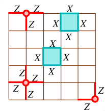
Figure 1: Stabilizer generators for the planar code state $|K\rangle$. Qubits are located on the edges of the lattice. $Z$-type stabilizer generators live on vertices, and $X$-type stabilizer generators live on plaquettes.

It is worthwhile to write down the state $|K\rangle$ explicitly. We shall use the computational basis of ${\cal H}$. Accordingly, a basis vector $|x\rangle$ represents a configuration of $N_{1}$ binary variables $x=\{x_{e}\}_{e=1,\ldots,N_{1}}$, $x_{e}\in\{0,1\}$ living at the edges of the lattice. We shall call such a configuration a $1$-chain. Let us call a $1$-chain $x$ a $1$-cycle iff $\sum_{e\in\delta s}x_{e}$ is even for every vertex $s$. In other words, a $1$-cycle must have even number of edges incident to any vertex. Let ${\cal Z}\subset\{0,1\}^{N_{1}}$ be a set of all $1$-cycles. Then the state $|K\rangle$ can be explicitly written in the computational basis as

$$|K\rangle=\frac{1}{\sqrt{|{\cal Z}|}}\,\sum_{x\in{\cal Z}}|x\rangle.$$ (3)

One can easily check that $|{\cal Z}|=2^{N_{2}}$, that is each plaquette contributes one independent $1$-cycle to ${\cal Z}$.

MQC with the planar code state is defined as adaptive sequence of one-qubit measurements $M_{1},M_{2},\ldots,M_{N_{1}}$ applied to the state $|K\rangle$. After all measurements are done, every qubit on the lattice is measured in some basis. The choice of the measurement $M_{j+1}$ may be determined by the outcomes of all earlier measurements $M_{1},\ldots,M_{j}$. We allow only complete von Neumann measurements. In other words, $M_{j}$ is specified by a unity decomposition

$$I=|\psi_{j}^{0}\rangle\langle\psi_{j}^{0}|+|\psi_{j}^{1}\rangle\langle\psi_{j}^{1}|$$

for some orthonormal basis $|\psi_{j}^{0}\rangle,|\psi_{j}^{1}\rangle\in\mathbb{C}^{2}$. Let $e_{j}$ denote the qubit to be measured at step $j$ and $m_{j}\in\{0,1\}$ be the outcome of the measurement $M_{j}$. After the measurement the qubit $e_{j}$ is projected onto a state $|\psi_{j}^{m_{j}}\rangle$. Thus MQC is specified by

• Description of the first measurement
  $M_{1}=(e_{1},|\psi_{1}^{0}\rangle,|\psi_{1}^{1}\rangle)$

• Efficient algorithm that takes as input outcomes $m_{1},\ldots,m_{j}$ of the first $j$ measurements and returns a description of the next measurement
  $M_{j+1}=(e_{j+1},|\psi_{j+1}^{0}\rangle,|\psi_{j+1}^{1}\rangle)$.

The output of MQC is a string of outcomes $m_{1},\ldots,m_{N_{1}}$ having some probability distribution $p(m_{1},\ldots,m_{N_{1}})$. We say that MQC can be efficiently simulated classically if there exists a classical randomized algorithm running in a time $poly(L)$ that allows one to sample $m_{1},\ldots,m_{N_{1}}$ from the probability distribution $p(m_{1},\ldots,m_{N_{1}})$.

In general, there are no restrictions on the order in which the qubits are measured in MQC. We shall consider more restrictive settings (because our technique does not apply to the general case). Consider a set $E_{j}=(e_{1},e_{2},\ldots,e_{j})$ including all qubits measured up to the step $j$ of MQC. Let $\bar{E}_{j}$ be the complimentary set including all unmeasured qubits. Let us say that a set of edges $E$ is connected iff for any pair of edges $e,e^{\prime}\in E$ there exists a path $e_{0}=e,e_{1},e_{2},\ldots,e_{n}=e^{\prime}$ that connects $e$ with $e^{\prime}$ and such that $e_{l}\in E$ for all $l$. Our main result is

Theorem.

Suppose at each step $j=1,\ldots,N_{1}$ of MQC the sets of measured and unmeasured qubits $E_{j}$, $\bar{E}_{j}$ are connected. Then MQC can be efficiently simulated classically.

The proof relies on two observations. The first observation made by Kitaev Kitaev-pc is that the overlap problem — computing the inner product between $|K\rangle$ and an arbitrary product state can be reduced to computing partition function of the Ising model with complex weights. The connection between overlaps of states and partition functions of models in statistical mechanics is explored in greater generality in VdN2 .

More strictly, we use Barahona’s techniques Barahona81 to express the overlap as a generating function of perfect matchings on a properly defined planar graph. It was shown by Kasteleyn Kasteleyn61 that such generating functions can be computed efficiently, see Galluccio98 for more recent exposition. Thus if every qubit on the lattice is measured in some specified basis, probability of any particular outcome can be computed efficiently.

However, this observation solves only part of the problem. First of all, since the number of possible outcomes, $2^{N_{1}}$, is exponentially large, computing probability of any particular outcome does not allow us to sample the outcomes according to these probabilities. More importantly, since the measurements in MQC are adaptive, we must be able to compute probabilities of partial measurements, when only some subset of qubits is measured. Our second observation is that the overlap problem for a subset of qubits can be reduced to computing partition function of the Ising model for two independent replicas of the lattice with properly identified boundaries. The constraint that the subsets $E_{j},\bar{E_{j}}$ are connected is the simplest way to ensure that the doubled lattice corresponds to a planar graph. The partition function of Ising model on any planar graph can be computed efficiently using Barahona’s algorithm Barahona81 . Given probabilities of any partial measurement outcomes, we can compute conditional probabilities and thus we can simulate MQC.

Whether or not the connectivity constraint is a severe restriction on MQC is an open question. Note that this constraint is trivially satisfied in the standard scheme of MQC, when the qubits are measured in the order “from the left to the right”. We also conjecture that the theorem above can be generalized to the following scenarios: (1) the number of connected components in $E_{j},\bar{E}_{j}$ is greater than one, but can be bounded by a constant. (2) The square lattice on a plane can be replaced by a lattice on any two-dimensional orientable surface with genus $g$ bounded by a constant. The intuition supporting these conjectures comes from the work Galluccio98 providing an efficient algorithm to compute the generating function of perfect matching if the genus of the graph can be bounded by a constant.

III Classical simulation

This section is organized as follows. Section III.1 describes the reduction from the overlap problem to the Ising model and then to the perfect matchings on a planar graph. It mainly follows the reference Barahona81 (except for considering complex weights) and aims to make our exposition self-sufficient. Section III.2 shows how to describe a mixed state obtained from $|K\rangle$ by the partial trace over a subset of qubits as a mixture of planar code states. Finally, Section III.3 explains how to compute probability of any partial measurement outcome by taking two copies of the lattice.

III.1 The overlap between planar code states and product states

In this section we consider planar code states on subgraphs of the square lattice . We show that the overlap (the inner product) between the planar code state and a product of any one-qubit states can be efficiently computed using techniques developed by Kasteleyn and Barahona Kasteleyn61 ; Barahona81 .

Suppose the planar code state $|K\rangle$ is defined on a square lattice ${\cal L}$, see Figure 1. Denote $V({\cal L})$ and $E({\cal L})$ sets of vertices and edges of ${\cal L}$. For any subset of edges $E\subseteq E({\cal L})$ define a planar graph $G_{E}=(V,E)$, where $V\subseteq V({\cal L})$ is a set of all vertices $s\in V({\cal L})$ having at least one incident edge from $E$,

$$V=\{s\in V({\cal L})\,:\,\delta s\cap E\neq\emptyset\}.$$

We shall denote $C_{1}(E)$ a set of $1$-chains on the subset $E$.

Let qubits live on edges $e\in E$. Accordingly, the Hilbert space is now $(\mathbb{C}^{2})^{\otimes|E|}$, and basis vectors correspond to $1$-chains $x\in C_{1}(E)$. We shall consider a set of $1$-cycles

$${\cal Z}(E)=\{x\in C_{1}(E)\,:\,\sum_{e\in\delta s\,\cap E}x_{e}\;\mbox{is even for all $s\in V$}\}.$$ (4)

For brevity, we shall keep using notation ${\cal Z}\equiv{\cal Z}(E)$ throughout this section. Define a planar code state $|G_{E}\rangle$ associated with the graph $G_{E}$ as

$$|G_{E}\rangle=\frac{1}{\sqrt{|{\cal Z}|}}\,\sum_{x\in{\cal Z}}|x\rangle.$$ (5)

Note that $|{\cal Z}|$ can be computed efficiently since ${\cal Z}$ is specified by mod-$2$ linear equations.

Consider an arbitrary product state

$$|\Phi\rangle=\bigotimes_{e\in E}|\phi_{e}\rangle,\quad|\phi_{e}\rangle=\alpha_{e}\,|0\rangle+\beta_{e}\,|1\rangle.$$

The quantity we are interested in is the overlap between $|\Phi\rangle$ and $|G_{E}\rangle$,

$$\Gamma=\langle G_{E}|\Phi\rangle=|{\cal Z}|^{-\frac{1}{2}}\,\prod_{e\in E}\alpha_{e}\sum_{x\in{\cal Z}}\;\prod_{e\in E\,:\,x_{e}=1}\left(\frac{\beta_{e}}{\alpha_{e}}\right).$$

This expression becomes singular if $\alpha_{e}=0$ for some $e$. The singularity can be avoided by assigning small non-zero value to $\alpha_{e}$ and using continuity of $\Gamma$ as a function of $\alpha$’s and $\beta$’s (see also ). For every edge $e\in E$ define a complex weight $w_{e}=\beta_{e}/\alpha_{e}$. Then $\Gamma$ is proportional to a “partition function”

$$Z=\sum_{x\in{\cal Z}}\;\prod_{e\in E\,:\,x_{e}=1}w_{e}.$$ (6)

Let us mention that $Z$ can be identified with a partition function of the Ising model with complex weights. Indeed, introduce virtual Ising spins $\sigma_{f}=\pm 1$ living on faces $f$ of $G_{E}$ and use the ansatz $1-2x_{e}=\sigma_{f}\sigma_{g}$, where $f$ and $g$ are the two faces of $G_{E}$ whose boundary includes the edge $e$. Then any choice of variables $\sigma_{f}$ automatically satisfies the $1$-cycle constraint $x\in{\cal Z}$. Besides, $w_{e}^{x_{e}}=\sqrt{w_{e}}\,\exp{(-\beta_{f,g}\,\sigma_{f}\sigma_{g})}$, where $e^{\beta_{f,g}}=\sqrt{w_{e}}$. Thus $Z$ is proportional to the partition function of the Ising models with Ising spins living on faces of $G_{E}$. In fact, the reverse reduction from the Ising model to the model described by Eq. (6) is the first step in Barahona’s solution of the Ising model Barahona81 . Since some arguments in Barahona’s original work assume that the weights $w_{e}$ are real and positive, we shall briefly explain how to apply the same approach to complex weights. (Note that in general partition functions with complex weights are more difficult to compute because of the sign problem.)

Since $G_{E}$ is a subgraph of the square lattice, vertices of $G_{E}$ may have degree (number of incident edges) $1,2,3$, or $4$. Let us firstly get rid of vertices with degree $1,2,4$. Suppose $s\in V$ has degree $1$ and $e$ is the edge incident to $s$. Clearly, $x_{e}=0$ for any $1$-cycle $x\in{\cal Z}$. Thus $Z$ does not depend on $w_{e}$ and we can safely remove the edge $e$ from the graph. Now we can assume that all vertices of $G_{E}$ have degree $2,3$, or $4$. Suppose $s\in V$ has degree $2$ and $e_{1}$, $e_{2}$ are the two edges incident to $s$. Clearly, $x_{e_{1}}=x_{e_{2}}$ for any $1$-cycle $x\in{\cal Z}$. Therefore we can remove the vertex $s$ and merge the edges $e_{1}$, $e_{2}$ into a single edge $e$ with a weight $w_{e}=w_{e_{1}}w_{e_{2}}$. Now we can assume that all vertices of $G_{E}$ have degree $3$ or $4$. Suppose $s\in V$ has degree $4$. Following Barahona81 let us replace $s$ by two vertices $s_{1}$, $s_{2}$ of degree $3$ by adding a new edge $e=(s_{1},s_{2})$ with a weight $w_{e}=1$, see Figure 2. If $e_{1},e_{2},e_{3},e_{4}$ are the edges incident to $s$, see Figure 2, and $x\in{\cal Z}$ is a $1$-cycle, then $x_{e_{1}}+x_{e_{2}}+x_{e_{3}}+x_{e_{4}}=0$ (we use mod-$2$ arithmetics). After adding a new edge $e$ we get $x_{e}=x_{e_{1}}+x_{e_{4}}=x_{e_{2}}+x_{e_{3}}$. Thus there is one-to-one correspondence between $1$-cycles on the original and the modified graph. Since $w_{e}=1$, the partition functions Eq. (6) are the same for both graphs. Now we can assume that all vertices of $G_{E}$ have degree $3$.

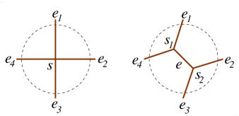
Figure 2: Local modification of the graph proposed by Barahona Barahona81 to eliminate degree-$4$ vertices. The two graphs coincide outside the dashed circle. The added edge $e$ carries trivial weight $w_{e}=1$. The partition functions of the two graphs coincide.

Let $G=(V,E)$ be the $3$-valent planar graph that we obtained by performing all the reductions above (by abuse of notations, we use the same symbols $V$,$E$ for new set of vertices and edges). We want to compute the partition function Eq. (6) for the graph $G$. Following Barahona81 let us introduce a new planar graph $\tilde{G}=(\tilde{V},\tilde{E})$ such that each vertex $s\in V$ with incident edges $e_{1},e_{2},e_{3}\in E$ is replaced by $6$ vertices $s_{1},\ldots,s_{6}\in\tilde{V}$ and $6$ edges $e_{4},\ldots,e_{9}$ as shown on Figure 3. We assign trivial weights to all new edges, $w_{e_{4}}=\ldots=w_{e_{9}}=1$. A $1$-chain $y\in C_{1}(\tilde{E})$ is a perfect matching on the graph $\tilde{G}$ iff any vertex $s\in\tilde{V}$ has exactly one incident edge $e$ with $y_{e}=1$. Let ${\cal M}$ be a set of all perfect matchings on $\tilde{G}$. As was pointed out by Barahona Barahona81 , there is one-to-one correspondence ${\cal Z}(E)\cong{\cal M}$ between $1$-cycles on $G$ and perfect matching on $\tilde{G}$, in particular

$$Z=\sum_{x\in{\cal Z}}\;\prod_{e\in E\,:\,x_{e}=1}w_{e}=\sum_{y\in{\cal M}}\;\prod_{e\in\tilde{E}\,:\,y_{e}=1}w_{e}.$$ (7)

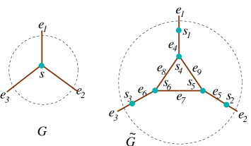
Figure 3: Local modification of the graph proposed by Barahona Barahona81 to reduce summation over $1$-cycles to summation over perfect matchings. The two graphs coincide outside the dashed circle. All six added edges $e_{4},\ldots,e_{9}$ carry trivial weight, $w_{e_{4}}=\ldots=w_{e_{9}}=1$. Any $1$-cycle $x\in{\cal Z}$ on the graph $G$ can be uniquely extended to a $1$-chain $y$ on $\tilde{G}$ such that $x$ and $y$ coincide outside the dashed circle (including the edges $e_{1},e_{2},e_{3}$) and such that $y$ is a perfect matching inside the dashed circle. Conversely, $y$ can not be a perfect matching if $y_{e_{1}}+y_{e_{2}}+y_{e_{3}}$ is odd.

By construction, $\tilde{G}$ has at least one perfect matching (the one corresponding to the zero $1$-cycle in $G$), and thus $\tilde{G}$ must have even number of vertices, $|\tilde{V}|=2m$.

Let $A$ be the adjacency matrix of the graph $\tilde{G}$, i.e., $A_{s,t}=1$ if $(s,t)\in\tilde{E}$ and $A_{s,t}=0$ otherwise. By definition, $A$ is symmetric, $A^{T}=A$. One can rewrite the summation over perfect matchings in Eq. (7) as

$$Z=\frac{1}{2^{m}\,m!}\sum_{\sigma\in S_{2m}}\,\prod_{j=1}^{m}A_{\sigma_{2j-1},\sigma_{2j}}\,w_{(\sigma_{2j-1},\sigma_{2j})},$$ (8)

where we label vertices of $\tilde{G}$ by integers $1,2,\ldots,2m$, where $\sigma$ is a permutation of the $2m$ vertices,

$$\sigma=\left(\begin{array}[]{ccccccc}1&2&3&4&\cdots&2m-1&2m\\ \sigma_{1}&\sigma_{2}&\sigma_{3}&\sigma_{4}&\cdots&\sigma_{2m-1}&\sigma_{2m}\\ \end{array}\right)$$

and $S_{2m}$ is the symmetric group.

Kasteleyn has shown Kasteleyn61 that for any planar graph it is possible to find antisymmetric matrix $B$ such that $B_{s,t}=\pm A_{s,t}$ for any pair of vertices $s,t$, $B^{T}=-B$, and such that $B$ obeys the Pfaffian orientation condition:

$$\prod_{j=1}^{m}B_{\sigma_{2j-1},\sigma_{2j}}=\mbox{sgn}\,{(\sigma)}\,\prod_{j=1}^{m}A_{\sigma_{2j-1},\sigma_{2j}}.$$

for any permutation $\sigma\in S_{2m}$. Here $\mbox{sgn}\,(\sigma)$ is the parity of $\sigma$. Define a complex antisymmetric $2m\times 2m$ matrix $B^{w}$ such that $B^{w}_{s,t}=B_{s,t}\,w_{(s,t)}$ if $(s,t)\in\tilde{E}$ and $B^{w}_{s,t}=0$ otherwise. Then the partition function Eq. (8) can be expressed as the Pfaffian of $B^{w}$,

$$Z=\frac{1}{2^{m}\,m!}\sum_{\sigma\in S_{2m}}\mbox{sgn}(\sigma)\,\prod_{j=1}^{m}B^{w}_{\sigma_{2j-1},\sigma_{2j}}=\mbox{Pf}\,(B^{w}).$$

Now it can be computed efficiently using the well-known identity $\mbox{Pf}\,(X)^{2}=\mbox{det}\,(X)$ valid for any complex antisymmetric matrix $X$.

III.2 Tracing out qubits from the planar code state

Suppose at some step $j$ of MQC a subset of qubits $E=\{e_{1},\ldots,e_{j}\}\subseteq E({\cal L})$ has been already measured. We want to show that a mixed state

$$\rho_{E}=\mbox{Tr}_{e\notin E}\,|K\rangle\langle K|$$

describing qubits from $E$ only (before the measurement) can be represented as a probabilistic mixture of pure states simply related to the planar code state $|G_{E}\rangle$, see Eq. (5).

Indeed, let $\bar{E}=E({\cal L})\backslash E$ be the set of traced out qubits. Denote $\bar{V}\subseteq V({\cal L})$ a set of vertices having at least one incident edge from $\bar{E}$, and $\partial E=V\cap\bar{V}$ be a set of vertices having at least one incident edge from both sets $E$, $\bar{E}$ (it can be regarded as a boundary of the set $E$). A $0$-chain on some set of vertices $M$ is a configuration of binary variables assigned to vertices of $M$, $u=\{u_{s}\}_{s\in M}$, $u_{s}\in\{0,1\}$. Let us denote $C_{0}(M)$ a set of all $0$-chains on $M$. Given any $1$-chain $x\in C_{1}(E)$, define a boundary $\partial x\in C_{0}(V)$ as a $0$-chain such that $(\partial x)_{s}$ is equal to the parity ($0$ or $1$) of edges $e$ incident to $s$ with $x_{e}=1$. Define a subspace of relative $1$-cycles

$${\cal Z}(E,\partial E)=\{x\in C_{1}(E)\,:\,(\partial x)_{s}=0\;\mbox{for all $s\notin\partial E$}\}.$$

Thus a relative $1$-cycle satisfies the $1$-cycle condition everywhere except (may be) of vertices $s\in\partial E$. Define a subspace of syndromes as

$${\cal S}(E)=\{u\in C_{0}(\partial E)\,:\,u=\partial z\;\;\mbox{for some $z\in{\cal Z}(E,\partial E)$}\}.$$

Simple linear algebra arguments show that any relative $1$-cycle $z\in{\cal Z}(E,\partial E)$ with a syndrome $u=\partial z\in{\cal S}(E)$ can be represented as $z=z(u)+x$, where $z(u)\in{\cal Z}(E,\partial E)$ is some fixed relative $1$-cycle satisfying $\partial z(u)=u$ and $x\in{\cal Z}(E)$ is $1$-cycle. Similarly, one can define a subspace of syndroms

$${\cal S}(\bar{E})=\{u\in C_{0}(\partial{E})\,:\,u=\partial\bar{z}\;\;\mbox{for some $\bar{z}\in{\cal Z}(\bar{E},\partial{E})$}\}.$$

Note that in general ${\cal S}(E)\neq{\cal S}(\bar{E})$. Any relative $1$-cycle $\bar{z}\in{\cal Z}(\bar{E},\partial E)$ with a syndrome $u=\partial\bar{z}\in{\cal S}(\bar{E})$ can be represented as $\bar{z}=\bar{z}(u)+y$, where $\bar{z}(u)\in{\cal Z}(\bar{E},\partial E)$ is some fixed relative $1$-cycle satisfying $\partial\bar{z}(u)=u$ and $y\in{\cal Z}(\bar{E})$ is a $1$-cycle.

The above definitions and arguments imply that a Schmidt decomposition of $|K\rangle$ with respect to the partition $E({\cal L})=E\cup\bar{E}$ can be chosen as follows:

$$|K\rangle=\frac{1}{\sqrt{|{\cal S}|}}\,\sum_{u\in{\cal S}}|G_{E}(u)\rangle\otimes|G_{\bar{E}}(u)\rangle,$$ (9)

where

$${\cal S}={\cal S}(E)\cap{\cal S}(\bar{E}),$$

$$|G_{E}(u)\rangle=\frac{1}{\sqrt{|{\cal Z}(E)|}}\,\sum_{x\in{\cal Z}(E)}\,|z(u)+x\rangle,$$

and

$$|G_{\bar{E}}(u)\rangle=\frac{1}{\sqrt{|{\cal Z}(\bar{E})|}}\,\sum_{y\in{\cal Z}(\bar{E})}\,|\bar{z}(u)+y\rangle,$$

Therefore we arrive at

$$\rho_{E}=\frac{1}{|{\cal S}|}\,\sum_{u\in{\cal S}}\,|G_{E}(u)\rangle\langle G_{E}(u)|.$$ (10)

III.3 Calculating probabilities of partial measurements

In this section we show how to compute the overlap $\langle\Phi|\rho_{E}|\Phi\rangle$, where $|\Phi\rangle$ is an arbitrary product state. At this point we shall exploit the constraint that $E$ and $\bar{E}$ are connected sets.

The first simplification arising from this constraint is that the subspace of syndromes ${\cal S}$ includes all even $0$-chains on the boundary $\partial E$:

$${\cal S}=\{u\in C_{0}(\partial E)\,:\,\sum_{s\in\partial E}u_{s}=0\,\mbox{(mod $2$)}\}.$$ (11)

Indeed, consider arbitrary even $0$-chain $u\in C_{0}(\partial E)$, and let $s_{1},s_{2},\ldots,s_{2k}\in\partial E$ be the set of vertices such that $u_{s_{j}}=1$. Consider firstly the pair of vertices $s_{1},s_{2}$. Since $s_{1},s_{2}\in\partial E$, there exist edges $e_{1},e_{2}\in E$ incident to $s_{1},s_{2}$ respectively (may be $e_{1}=e_{2}$). Since $E$ is a connected set, there exists a path $\gamma_{12}\subseteq E$ connecting $e_{1}$ and $e_{2}$. By definition, this path is a relative $1$-cycle, $\gamma_{12}\in{\cal Z}(E,\partial E)$ with the boundary $\partial\gamma_{12}$ supported on $s_{1}$ and $s_{2}$. Similarly, using the connectivity of $\bar{E}$, one can show that there exists a relative $1$-cycle $\bar{\gamma}_{12}\in{\cal Z}(\bar{E},\partial E)$ with the boundary $\partial\bar{\gamma}_{12}$ supported on $s_{1}$ and $s_{2}$. Repeating this arguments for the remaining pairs of vertices $(s_{3},s_{4}),\ldots,(s_{2k-1},s_{2k})$ we can construct relative $1$-cycles $z(u)=\gamma_{12}+\ldots+\gamma_{2k-1,2k}\in{\cal Z}(E,\partial E)$ and $\bar{z}(u)=\bar{\gamma}_{12}+\ldots+\bar{\gamma}_{2k-1,2k}\in{\cal Z}(\bar{E},\partial E)$ such that $\partial z(u)=u$ and $\partial\bar{z}(u)=u$. Thus $u\in{\cal S}$. Conversely, for any relative $1$-cycle $z\in{\cal Z}(E,\partial E)$ the boundary $\partial z$ must be even since $z$ consists of elementary edges and every edge has two endpoints. The same is true for relative $1$-cycles on $\bar{E}$. Therefore we have proved Eq. (11). It follows that $|{\cal S}|=2^{|\partial E|-1}$.

The next simplification that we draw from the connectivity of $E,\bar{E}$ is

Lemma.

Suppose $E,\bar{E}$ are connected sets. Then the graph $G_{E}$ can be drawn without intersections on a disk such that all vertices of $\partial E$ lie on the boundary of the disk.

Proof: Since $G_{E}$ is a planar graph, any point of the plane either belongs to $G_{E}$, or is ‘internal’ with respect to $G_{E}$, or is ‘external’ with respect to $G_{E}$. Denote $\mbox{Ext}\,(G_{E})$ a set of all external points. The fact that $E,\bar{E}$ are connected implies that (1) The boundary $\partial E$ is contained in the boundary of $\mbox{Ext}\,(G_{E})$; (2) The region $\mbox{Ext}\,(G_{E})$ is topologically equivalent to a plane with a hole. Therefore one can smoothly deform a plane such that after the deformation $G_{E}$ is contained in a disk and all points of $\partial E$ lie on the boundary of the disk. ∎

This lemma provides us with a way to compute the overlap $\langle\Phi|\rho_{E}|\Phi\rangle$. Indeed, consider two copies of the graph $G_{E}$ drawn on disjoint disks $D$ and $D^{*}$. Let us denote the two copies as $G_{E}$ and $G_{E}^{*}$. Let us glue the disks $D$, $D^{*}$ into a sphere such that vertices of the boundary $\partial E$ on the disk $D$ are glued with the corresponding vertices of the boundary $\partial E$ on the disk $D^{*}$. Denote the resulting graph $G_{E}\sqcup G_{E}^{*}$. Since $G_{E}\sqcup G_{E}^{*}$ can be drawn on a sphere, it is a planar graph and thus we can efficiently compute its partition function, as defined in Eq. (6). Let $w_{e}$ be a weight assigned to edge $e\in E$ on disk $D$. Let us assign the complex conjugated weight $w_{e}^{*}$ to the corresponding edge $e$ on the disk $D^{*}$. For any syndrome $u\in{\cal S}$ let $z(u)\in{\cal Z}(E,\partial E)$ be some fixed relative $1$-cycle such that $\partial z(u)=u$. Then the partition function for $G_{E}\sqcup G_{E}^{*}$ can be written as

$$Z(G_{E}\sqcup G_{E}^{*})=\sum_{u\in{\cal S}}\,|Z(u)|^{2},$$

where

$$Z(u)=\sum_{x\in{\cal Z}(E)}\,\;\prod_{e\in E\,:\,(z(u)+x)_{e}=1}\,w_{e}.$$

One can easily see that $Z(u)$ is equal to the overlap between a state $|G_{E}(u)\rangle$ in the decomposition Eq. (10) and a product state $|\Phi\rangle=\bigotimes_{e\in E}\,(|0\rangle+w_{e}\,|1\rangle)$, that is $Z(u)=\sqrt{|{\cal Z}(E)|}\,\langle G_{E}(u)|\Phi\rangle$. Therefore we conclude that

$$\langle\Phi|\rho_{E}|\Phi\rangle=\frac{1}{2^{|\partial E|-1}\,|{\cal Z}(E)|}\,Z(G_{E}\sqcup G_{E}^{*})$$

and thus the overlap can be computed efficiently using techniques from the previous section.

We can use the algorithm above for computing the overlap between $\rho_{E}$ and a product state to compute probabilities of any particular partial measurement outcomes $p(m_{1},\ldots,m_{j})$. It allows us to compute conditional probabilities $p(m_{j}\,||\,m_{1},\ldots,m_{j-1})$ for any $j=1,\ldots,N_{1}$. If we already know the outcomes $m_{1},\ldots,m_{j}$, we can sample $m_{j}$ from the probability distribution $p(m_{j}\,||\,m_{1},\ldots,m_{j-1})$. Thus all quantum steps in MQC can be efficiently simulated on a classical computer (with random numbers).

IV Extension to non-planar graphs

In this section we outline an MQC simulation scheme built around the planarity of graphs. It is complementary to the simulation scheme Shi1 - VandenNest06 via tensor networks, centered around the tree-ness of graphs. We identify a parameter $\eta$ which measures deviation from planarity and show that simulation of MQC is efficient in the number of particles in the resource state but exponentially inefficient in $\eta$.

In Section IV.1 it is shown that simulation based on planarity can not be subsumed under the tree tensor network method. In Section IV.2 we show that there is another interesting example among the states for which MQC can be related to the Ising model partition function: a universal 2D cluster state. The corresponding interaction graph (to be distinguished from the graph upon which the definition of graph states is based) is highly non-planar, such that simulation—as expected—is not efficient. In Section IV.3 we characterize the complexity of classical MQC simulation for non-planar Ising interaction graphs.

We would like to remark that the connection between the 1D cluster state and non-interacting fermions, a topic interwoven with the solvability of the Ising model on planar graphs, has previously been discussed in Pachos .

IV.1 The planar code state and tensor contraction

Here we show that a planar code state on a lattice of size $L\times L$ has an entanglement width of at least $L$ such that its simulation scheme based on a TTN is exponentially inefficient in $L$. See VdN2 for an alternative proof of this result.

The entanglement measure entanglement width has been defined in VdN1 and related to universality of MQC and to the complexity of its TTN-simulation in VdN1 ; VandenNest06 . We briefly restate the definition here. Consider a quantum system on a set $Q$ of qubits. Be $T$ a tree graph with each vertex having 1 or 3 incident edges (subcubic tree). The vertices with one edge are called leaves, and each of them corresponds to a qubit of the considered quantum system. If an edge $e$ is deleted from $T$, the resulting graph $T\backslash e$ has two connected components which induce a bi-partition $(A_{T}^{e},B_{T}^{e})$ of $Q$. For a pure state $|\psi\rangle$ we denote by $E_{A_{T}^{e},B_{T}^{e}}(|\psi\rangle)$ the entanglement entropy with respect to that bi-partition. The entanglement width is now defined as

$$E_{\text{wd}}(|\psi\rangle):=\min_{T}\max_{e}E_{A_{T}^{e},B_{T}^{e}}(|\psi\rangle),$$

where the minimization is over all subcubic trees with $n$ leaves, and the maximum over all edges $e$ in a given tree.

Lemma.

The entanglement width of a planar code state $|G_{L}\rangle$ on a square lattice of size $L\times L$ is

$$E_{\text{\em{wd}}}(|G_{L}\rangle)\geq L.$$ (12)

Proof: First we show that for any given subcubic tree $T$ with $|Q|$ leaves, there exists an edge $e$ such that $1/3\,|Q|\leq|A_{T}^{e}|,|B_{T}^{e}|\leq 2/3\,|Q|$. Given $T$, pick an arbitrary 3-valent vertex as root. This induces an ancestor-descendant relation among pairs of vertices. For each vertex $a\in V(T)$, denote by $n(a)$ the number of leaves among $a$ and all its descendants. There are vertices $a\in V(T)$ for which $n(a)>2/3n$. Among those, there must be a vertex $a_{0}$ such that for both its direct descendants $a_{1},a_{2}$ holds $n(a_{1}),n(a_{2})\leq 2/3\,n$. Choose $a_{1}$ s.th. $n(a_{1})\geq n(a_{2})$. The desired edge then is $e=(a_{0},a_{1})$. Be $A_{T}^{e}$ the set of qubits associated with the descendant leaves of $a_{1}$. Then, $|A_{T}^{e}|=n(a_{1})\leq 2/3\,n$. Also, $1/3\,n<n(a_{0})/2=(n(a_{1})+n(a_{2}))/2\leq n(a_{1})=|A_{T}^{e}|$.

Now, the entanglement entropy $E_{A_{T}^{e},B_{T}^{e}}$ is linear in the length of the boundary between $A_{T}^{e}$ and $B_{T}^{e}$ Zanardi04 . It is minimized if $A_{T}^{e}$ and $B_{T}^{e}$ are simply connected and use the external boundary of the $L\times L$ lattice. This occurs e.g. for $A_{T}^{e}$ filling up the bottom part of the lattice up to a certain height. The entanglement entropy in that case is $L$ or $L+1$. Thus, $\max_{e}E_{A_{T}^{e},B_{T}^{e}}(|G_{L}\rangle)\geq L$, for all subcubic trees $T$. ∎

The planar code state considered here is, like any other stabilizer state, local Clifford equivalent to a graph state Schling ; Grassl ; Hein . For graph states, the entanglement width equals the so-called rank width Oum of the underlying graph. The rank width $\chi$ is the critical parameter for the complexity of MQC simulation via tree tensor networks; the operational resources required in the simulation of an $n$-qubit system scale like $Poly(n,2^{\chi})$ VandenNest06 (c.f. Theorem 4 therein). Thus, MQC on $L\times L$-planar code states, with $\chi$ growing at least linearly in $L$, is not suited for efficient simulation by the methods developed in Shi1 - VandenNest06 .

IV.2 The 2D cluster state in the Ising model

There is a two-dimensional universal cluster state associated with an edge-centered graph (see Fig. 4a) whose overlap with an arbitrary product state is described by the Ising model partition function. However, its interaction graph is not planar.

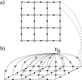
Figure 4: Universal graph state and its surface code representation. a) The two-dimensional cluster state $|{\cal{C}}_{L}\rangle$, for $L=3$. Qubits are located on the vertices $\bullet$, $\odot$. b) Local unitary equivalent surface code state $|\tilde{G}_{L}\rangle$. Here, qubits are located on the edges, and state stabilizers are associated with the sites and the plaquettes. To better illustrate the identification of qubits in $|\tilde{G}_{L}\rangle$ with their counterparts in $|{\cal{C}}_{L}\rangle$, the edges of $\tilde{G}_{L}$ are labeled by the same symbols as the vertices in ${\cal{C}}_{L}$. The dashed lines indicate pairs of corresponding qubits.

The cluster state $|{\cal{C}}_{L}\rangle$ under consideration is shown in Fig. 4 a. Qubits are associated with the vertices of the displayed graph ${\cal{C}}_{L}$. The stabilizer of ${\cal{C}}_{L}$ is generated by the Pauli operators

$$K_{a}=X_{a}\bigotimes_{b|\,(a,b)\in E({\cal{C}})}Z_{b},\;\;\forall a\in V({\cal{C}}_{L}).$$

The graph ${\cal{C}}_{L}$ is bi-colorable. We refer to the two colors as “$R$” and “$B$”, and use symbols “$\odot$” and “$\bullet$” to display the respective vertices. The cluster state $|{\cal{C}}_{L}\rangle$ is a universal resource for quantum computation Debbie .

Fig. 4b shows a surface code state $|\tilde{G}_{L}\rangle$ based on non-planar graph $\tilde{G}_{L}$. Qubits are associated with edges in $\tilde{G}_{L}$. $\tilde{G}_{L}$ is a modification of the previously discussed $L\times L$-lattice graph. It has one extra vertex $v_{0}$, extra edges $(v_{0},v_{i})$ and extra plaqettes $(v_{0},v_{i},v_{j})$, where $v_{i},v_{j}$ are vertices in the plane incident to a common edge. The stabilizer of $|\tilde{G}_{L}\rangle$ is spanned by the operators $A_{s}$, $B_{p}$ defined in Eq. (1). For an $L\times L$-lattice there are $N_{1}^{\prime}=2L(L+1)+(L+1)^{2}$ qubits, $N_{0}^{\prime}=(L+1)^{2}$ independent site- and $N_{2}^{\prime}=2L(L+1)$ independent plaquette stabilizers, and $|\tilde{G}_{L}$ is thus uniquely specified. $|\tilde{G}_{L}\rangle$ may again be written in the form of Eq. (5), and its overlap with a multi-local state may again, as in Eq. (6) be related to the partition function of the Ising model. However, the underlying interaction graph $\tilde{G}_{L}$ is now non-planar such that the techniques for efficient simulation Kasteleyn61 ; Barahona81 are no longer applicable.

The cluster state $|{\cal{C}}_{L}\rangle$ and surface code state $|\tilde{G}_{L}\rangle$ are local unitary equivalent. First, they have support on the same number of qubits, and we can pairwise identify the respective qubit locations. The mapping is as follows. The vertices of color $R$ in ${\cal{C}}$ reappear as vertices of $\tilde{G}_{L}$, but they are no longer qubit locations. As for the latter, each $R$-colored vertex $v$ of ${\cal{C}}_{L}$ corresponds to an edge $(v,v_{0})$ of $\tilde{G}_{L}$ above the plane, and each $B$-colored vertex $v^{\prime}$ of ${\cal{C}}_{L}$, located between two $R$-colored vertices $v_{1}$, $v_{2}$, corresponds to the edge $(v_{1},v_{2})$ of $\tilde{G}_{L}$ inside the plane; See Fig. 4. Denote by $H_{R}$ the simultaneous local Hadamard transformation on all qubits of color $R$. Then, $|\tilde{G}_{L}\rangle=H_{R}|\phi\rangle_{{\cal{C}}_{L}}$.

To see this, first consider the stabilizer $K_{w}$ of $|{\cal{C}}_{L}\rangle$ associated with a $B$-colored qubit location $w$, $K_{w}=X_{w}Z_{v_{1}}Z_{v_{2}}$ ($v_{1},\,v_{2}$ are vertices of color $R$). Under the identification of vertices in ${\cal{C}}_{L}$ with edges in $\tilde{G}_{L}$, $v_{1,2}\leftrightarrow(v_{0},v_{1,2})$, $w\leftrightarrow(v_{1},v_{2})$. (Again, $v_{0}$ is the extra vertex above the code plane.) After application of $H_{R}$, the operator $K_{w}$ is mapped to $X_{(v_{1},v_{2})}X_{(v_{0},v_{1})}X_{(v_{0},v_{2})}=B_{p}$ for $p=(v_{0},v_{1},v_{2})$; c.f. Eq. (1). Second, consider the stabilizer $K_{v}$ for an $R$-colored vertex $v\in V({\cal{C}}_{L})$, $K_{v}=X_{v}\otimes_{w|\,(v,w)\in E({\cal{C}})}Z_{w}$. With the identification $v\leftrightarrow(v,v_{0})$, $w\leftrightarrow(v,w)$, and after application of $H_{R}$, the stabilizer $K_{v}$ is mapped onto $Z_{(v,v_{0})}\otimes_{w|(v,w)\in E(\tilde{G}_{L})}Z_{(v,w)}=A_{v}$. ∎

The overlap between a local state $|\Phi\rangle=\bigotimes_{e\in\tilde{E}}|\phi_{e}\rangle$ and $|\tilde{G}_{L}\rangle$ may again be written as the partition function of the Ising model,

$$\ \begin{array}[]{rcl}\displaystyle{\langle\tilde{G}_{L}|\Phi\rangle}&\sim&\displaystyle{\sum_{\{\sigma_{j}\}}\exp\left(\sum_{(j,k)}\beta_{jk}\sigma_{j}\sigma_{k}\right)}\\ &\sim&\displaystyle{\sum_{\{\sigma_{j}|j\neq v_{0}\}}\!\!\!\!\exp\left(\sum_{(jk)|j,k\neq v_{0}}\!\!\!\!\!\beta_{jk}\sigma_{j}\sigma_{k}+\sum_{j\neq v_{0}}\!\!\beta_{j0}\sigma_{j}\right).}\end{array}$$ (13)

Therein, the $\beta_{jk}$ are specified through the relation $\exp(\beta_{jk})=\sqrt{\langle 0|\tilde{\phi}_{jk}\rangle/\langle 1|\tilde{\phi}_{jk}\rangle}$, and $|\tilde{\phi}_{e}\rangle=H_{e}\,|\phi_{e}\rangle$. As can be seen from the lower line in Eq. (13), the overlap between a local state and a universal 2D cluster state corresponds to the partition function of the planar Ising model in the presence of a magnetic field.

IV.3 The complexity of MQC simulation for non-planar interaction graphs

First, we would like to morph the simulation of MQC with a planar code state into simulation of MQC with the universal cluster state, by ‘switching on magnetic fields’. This may be performed gradually, switching on one magnetic field at a time. Fig. 5 shows the graph corresponding to an intermediate state of this sequence. The sequence is passed in reverse order if one starts from a 2D cluster state of Fig. 4 and measures, one by one, the cluster qubits of color $R$ in the $X$-basis. More generally, $X$- and $Z$-measurements directly operate at the level of Ising interaction graphs $\tilde{G}$; by deletion and contraction of edges, respectively.

A measure for deviation from a planar graph is the number $\eta$ of edges that needs to be deleted from a graph to make it planar. This parameter $\eta$ also governs the complexity of a straightforward extension of the simulation scheme presented in Section III, applicable to non-planar graphs. Be $E_{\text{np}}$ a set of edges in $\tilde{G}$ such that $\tilde{G}\backslash E_{\text{np}}$ is planar. Then, the product state $\bigotimes_{e\in E_{\text{np}}}|\phi_{e}\rangle$ may be expanded into the $X$-basis and the efficient simulation of MQC on the remaining planar graph may be run for each component. The operational cost of this simulation method for an $n$-qubit state $|\tilde{G}\rangle$ is $Poly(n)2^{\eta}$, which may be compared to Theorem 4 of VandenNest06 for tree tensor networks.

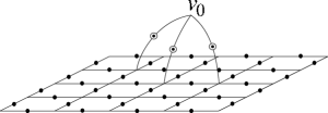
Figure 5: Intermediate state between the planar code state and a two-dimensional cluster state.

V Conclusion

We have shown that the overlap between the planar code state and any product state can be computed efficiently classically, through its correspondence with the planar Ising model. Under rather general assumptions about the pattern of one-qubit measurements, MQC with the planar code state as a quantum resource is not universal. It can be efficiently simulated on a classical computer. MQC with a universal 2D cluster state can also be related to the Ising model. However, the corresponding interaction graph is non-planar.

- (1) R. P. Feynman, Int. J. Theor. Phys. 21, 467 (1982); Opt. News 11, 11 (1985); Found. Phys. 16, 507 (1986).
- (2) G. Vidal, Phys. Rev. Lett. 93, 040502 (2004).
- (3) R. Cleve, A. Ekert, Ch. Macchiavello, M. Mosca, Proceedings of the Royal Society of London, Series A 454, No. 1969, 339 (1998).
- (4) G. Giedke and J.I. Cirac, Phys. Rev. A 66, 032316 (2002).
- (5) S. Bravyi, Quant. Inf. Comp. 5, Vol. 3, 216 (2005).
- (6) B.M. Terhal and D.P. DiVincenzo, Phys. Rev. A 65, 032325 (2002).
- (7) D. Gottesman, Proceedings of the XXII International Colloquium on Group Theoretical Methods in Physics, 32 (1999).
- (8) R. Raussendorf and H.-J. Briegel, Phys. Rev. Lett. 86, 5188 (2001).
- (9) N. de Beaudrap, V. Danos, E. Kashefi, quant-ph/0603266.
- (10) W. Hall, quant-ph/0512130.
- (11) D. Gross and J. Eisert, quant-ph/0609149.
- (12) A.M. Childs, D.W. Leung, M.A. Nielsen, Phys. Rev. A 71, 032318 (2005).
- (13) M. van den Nest, A. Miyake, W. Dür and H.-J. Briegel, Phys. Rev. Lett 97, 150504 (2006).
- (14) I. Markov, Y.-Y. Shi, quant-ph/0511069.
- (15) Y.-Y. Shi, L.-M. Duan and G. Vidal, quant-ph/0511070.
- (16) M. Van den Nest, W. Dür, G. Vidal, and H. J. Briegel, quant-ph/0608060.
- (17) M.A. Nielsen, quant-ph/0504097.
- (18) A. Kitaev, Ann Phys. (N.Y.) 303, 2 (2003).
- (19) S. Bravyi and A. Kitaev, quant-ph/9811052.
- (20) R. Raussendorf, S. Bravyi and J. Harrington, Phys. Rev. A 71, 062313 (2005).
- (21) E. Dennis, A. Kitaev, A. Landahl, J. Preskill, J. Math. Phys. 43, 4452 (2002).
- (22) A. Hamma, R. Ionicioiu, and P. Zanardi, Phys. Lett. A 337, 22 (2005).
- (23) S. Bravyi, M. B. Hastings, and F. Verstraete, Phys. Rev. Lett. 97, 050401 (2006).
- (24) A. Kitaev, private communication (2005).
- (25) M. van den Nest, W. Dür and H.-J. Briegel, quant-ph/0610157.
- (26) F. Barahona, J. Phys. A: Math. Gen. 15, 3241 (1982).
- (27) P. Kasteleyn, Physica 27, 1209 (1961).
- (28) A. Galluccio and M. Loebl, Electron. J. Combinat. 6, R6 (1999).
- (29) J.K. Pachos, M.B. Plenio, Phys. Rev. Lett. 93, 056402 (2004).
- (30) D. Schlingemann, R.F. Werner, Phys. Rev. A 65, 012308 (2002).
- (31) M. Grassl, A. Klappenecker and M. Rötteler, IEEE international symposium on information theory, Lausanne (2001).
- (32) M. Hein et al., Proceedings of the International School of Physics “Enrico Fermi” on “Quantum Computers, Algorithms and Chaos”, Varenna, Italy (2005); quant-ph/0602096.
- (33) S.-I. Oum, PhD-thesis, Princeton University (2005).