Displacement deformed quantum fields

Abstract

A displacement operator $\hat{d}_{\zeta}$ is introduced, verifying commutation relations $[\hat{d}_{\zeta},a_{f}^{\dagger}]=[\hat{d}_{\zeta},a_{f}]=\zeta(f)\hat{d}_{\zeta}$ with field creation and annihilation operators that verify $[a_{f},a_{g}]=0$, $[a_{f},a_{g}^{\dagger}]=(g,f)$, as usual. $f$ and $g$ are test functions, $\zeta$ is a Poincaré invariant real-valued function on the test function space, and $(g,f)$ is a Poincaré invariant Hermitian inner product. The $\star$-algebra generated by all these operators, and a state defined on it, nontrivially extends the $\star$-algebra of creation and annihilation operators and its Fock space representation. If the usual requirement for linearity is weakened, as suggested in quant-ph/0512190, we obtain a deformation of the free quantum field.

1 Introduction

In an earlier paper, I introduced a weakening of the axioms of quantum field theory that allows a nonlinear inner product structure [1]. I refer to that paper for notation, motivation, and an introduction to the approach that is further pursued here. There, I mentioned that I had investigated deformations of the Heisenberg algebra of the Arik-Coons type [2], but had found no way to apply deformations of a comparable type to quantum fields. Here, I briefly describe the failure, and move on to introduce a displacement operator $\hat{d}_{\zeta}$, verifying $[\hat{d}_{\zeta},a_{f}^{\dagger}]=[\hat{d}_{\zeta},a_{f}]=\zeta(f)\hat{d}_{\zeta}$, where $\zeta$ is an arbitrary real-valued scalar function on the test function space (taken to be a Schwartz space [3, §II.1]), which will allow us to construct an extension of Fock space, generated by the action of displacement operators on a vacuum state as well as by the action of creation operators $a_{f}^{\dagger}$. Note that the “displacement” is not a space-time displacement, but will shortly be seen to “displace” creation and annihilation operators in the sense of adding a scalar. What follows will show some of the uses to which such operators can be put.

A comparable (but Hermitian) number operator $\hat{n}_{\zeta}$ would verify the very different commutation relation $[\hat{n}_{\zeta},a_{f}^{\dagger}]=\zeta(f)a_{f}^{\dagger}$. Number operators are important for a uniform presentation of algebras of the Arik-Coons type[2], but we cannot in general construct an associative algebra if we use the operator $\hat{n}_{\zeta}$ to extend the free quantum field algebra ; it is straightforward to verify, for example, that for the undeformed commutation relation $[a_{f},a_{g}^{\dagger}]=(g,f)$, $\hat{n}_{\zeta}a_{f}a_{g}^{\dagger}$ becomes either $(a_{g}^{\dagger}a_{f}+(g,f))(\hat{n}_{\zeta}-\zeta(f)+\zeta(g))$ or $a_{g}^{\dagger}a_{f}(\hat{n}_{\zeta}-\zeta(f)+\zeta(g))+(g,f)\hat{n}_{\zeta}$, depending on the order in which the commutation relations are applied, which is incompatible with associativity unless $\zeta$ is a constant function on the test function space. We will here take the constant function number operator to be relatively uninteresting, particularly because we cannot generate an associative algebra using both a number operator $\hat{n}_{1}$ (with the constant function $1$) and a displacement operator $\hat{d}_{\zeta}$ ; $\hat{d}_{\zeta}\hat{n}_{1}a_{f}^{\dagger}$, for example, becomes different values depending on the order in which commutation relations are applied. Equally, every attempt I have made at deforming the commutation relations $[a_{f},a_{g}^{\dagger}]=(g,f)$ and $[a_{f},a_{g}]=0$ using number operators or displacement operators have failed to be associative, with $a_{f}(a_{h}a_{g}^{\dagger})\not=a_{h}(a_{f}a_{g}^{\dagger})$.

We will work with a $\star$-algebra $\mathcal{A}_{1}$ that is generated by creation and annihilation operators that verify $[a_{f},a_{g}^{\dagger}]=(g,f)$ and $[a_{f},a_{g}]=0$, together with a single displacement operator pair $\hat{d}_{\zeta}$ and $\hat{d}_{\zeta}^{\dagger}$. We will take $\hat{d}_{\zeta}^{\dagger}$ to be equivalent to $\hat{d}_{-\zeta}$; $\hat{d}_{\zeta}^{k}$ to be equivalent to $\hat{d}_{k\zeta}$; and $\hat{d}_{0\zeta}$ to be equivalent to $1$. The commutation relations above and the state we will define in a moment are consistent with these equivalences. $\hat{d}_{0\zeta}$ is central in $\mathcal{A}_{1}$, for example. In general, we will take $\hat{d}_{m\zeta}\hat{d}_{n\zeta}$ to be equivalent to $\hat{d}_{(m+n)\zeta}$.

$\mathcal{A}_{1}$ has the familiar subalgebra $\mathcal{A}_{0}$ that is generated by the creation and annihilation operators alone. A basis for $\mathcal{A}_{1}$ is $a_{g_{1}}^{\dagger}a_{g_{2}}^{\dagger}...a_{g_{m}}^{\dagger}\hat{d}_{k\zeta}a_{f_{1}}a_{f_{2}}...a_{f_{n}}$, $k\in{\mathrm{ZZ}}$, for some set of test functions $\{f_{i}\}$. We construct a linear state $\varphi_{0}$ on this basis as

$$\varphi_{0}(1)=1,$$ (1)

$$\varphi_{0}(a_{g_{1}}^{\dagger}a_{g_{2}}^{\dagger}...a_{g_{m}}^{\dagger}\hat{d}_{k\zeta}a_{f_{1}}a_{f_{2}}...a_{f_{n}})=0\quad\mathrm{if}\ m>0\ \mathrm{or}\ n>0\ \mathrm{or}\ k\not=0.$$ (2)

If $k$ is always zero, this is exactly the vacuum state for the conventional free quantum field. To establish that $\varphi_{0}$ is a state on $\mathcal{A}_{1}$, we have to show that $\varphi_{0}(\hat{A}^{\dagger}\hat{A})\geq 0$ for every element of the algebra. A general element of the algebra can be written as $\hat{A}=\sum_{k}\sum_{r}\lambda_{kr}\hat{X}^{\dagger}_{kr}\hat{d}_{k\zeta}\hat{Y}_{kr}$, where $\hat{X}_{kr}$ and $\hat{Y}_{kr}$ are products of annihilation operators, so that

$$\varphi_{0}(\hat{A}^{\dagger}\hat{A}) = \varphi_{0}((\sum_{j}\sum_{s}\lambda_{js}^{*}\hat{Y}^{\dagger}_{js}\hat{d}_{-j\zeta}\hat{X}_{js})(\sum_{k}\sum_{r}\lambda_{kr}\hat{X}^{\dagger}_{kr}\hat{d}_{k\zeta}\hat{Y}_{kr}))$$ (3)

$$= \sum_{k}\varphi_{0}((\sum_{s}\lambda_{js}^{*}\hat{Y}^{\dagger}_{js}{\hat{X}}^{\prime}_{js})(\sum_{r}\lambda_{kr}\hat{X^{\prime}}^{\dagger}_{kr}\hat{Y}_{kr}))$$ (4)

$$= \sum_{k}\varphi_{0}(\hat{A}_{k}^{\dagger}\hat{A}_{k})\geq 0,$$ (5)

because only terms for which $j=k$ contribute, and $\hat{A}_{k}=\sum_{r}\lambda_{kr}\hat{X^{\prime}}^{\dagger}_{kr}\hat{Y}_{kr}$ is an operator in the free quantum field algebra $\mathcal{A}_{0}$ for each $k$. The critical observation is that ${\hat{X}}^{\prime}_{kr}=\hat{d}_{-k\zeta}\hat{X}_{kr}\hat{d}_{k\zeta}$ is a sum of products of annihilation operators only.

Given the state $\varphi_{0}$, we can use the GNS construction to construct a Hilbert space $\mathcal{H}_{0}$ (see, for example, [3, §III.2]), then we can use the $C^{\star}$-algebra of bounded operators $\mathcal{B}(\mathcal{H}_{0})$ that act on $\mathcal{H}_{0}$ as an algebra of observables, but this or a similar construction is not strictly needed for Physics. From the point of view established in [1], we can be content to use a finite number of creation operators and annihilation operators to generate a $\star$-algebra of operators. This is not enough to support a continuous representation of the Poincaré group, but the formalism is Poincaré invariant, adequate (if we take enough generators) to construct complex enough models to be as empirically adequate as a continuum limit, and is much simpler, more constructive, and more appropriate for general use than Type $\mathrm{III}_{1}$ von Neumann algebras. This paper broadly follows the general practice in physics of fairly freely employing unbounded creation and annihilation operators. Completion of a $\star$-algebra in a norm to give at least a Banach $\star$-algebra structure, which would allow us to construct an action on the GNS Hilbert space directly, is a useful nicety for mathematics, but it is not essential for constructing physical models.

For future reference, I list some of the simplest identities that are entailed by the commutation relation of the displacement operator with the creation and annihilation operators (using a Baker-Campbell-Hausdorff (BCH) formula for the exponentials):

$$[\hat{d}_{\zeta}^{k},a_{f}^{\dagger}]=[\hat{d}_{\zeta}^{k},a_{f}]=k\zeta(f)\hat{d}_{\zeta}^{k},$$ (6)

$$\hat{d}_{\zeta}^{k}a_{f}^{\dagger}=(a_{f}^{\dagger}+k\zeta(f))\hat{d}_{\zeta}^{k},\qquad\hat{d}_{\zeta}^{k}e^{i\lambda a_{f}^{\dagger}}=e^{i\lambda(a_{f}^{\dagger}+k\zeta(f))}\hat{d}_{\zeta}^{k},$$ (7)

$$\hat{d}_{\zeta}^{k}a_{f}=(a_{f}+k\zeta(f))\hat{d}_{\zeta}^{k},\qquad\hat{d}_{\zeta}^{k}e^{i\lambda a_{f}}=e^{i\lambda(a_{f}+k\zeta(f))}\hat{d}_{\zeta}^{k},$$ (8)

$$e^{\alpha\hat{d}_{\zeta}-\alpha^{*}\hat{d}_{\zeta}^{\dagger}\,}a_{f}=\left[a_{f}+\zeta(f)(\alpha\hat{d}_{\zeta}+\alpha^{*}\hat{d}_{\zeta}^{\dagger})\right]e^{\alpha\hat{d}_{\zeta}-\alpha^{*}\hat{d}_{\zeta}^{\dagger}}.$$ (9)

From these it should begin to be clear why I have called $\hat{d}_{\zeta}$ a “displacement” operator. Equations (7) and (8) make apparent the useful practical consequence that it is sufficient to sum the powers of displacement operators in a term to be sure whether the term contributes to $\varphi_{0}(\hat{A})$ — if the sum of powers is zero — because displacement operators are not modified if they are moved to left or right in the term.

We can introduce as many displacement operators as needed, all mutually commuting, $[\hat{d}_{\zeta_{1}},\hat{d}_{\zeta_{2}}]=0$, without changing any essentials of the above, but probably not as far as a continuum of such operators without significant extra care. It is most straightforward to introduce linear dependency between products of the displacement operators immediately, $\hat{d}_{\zeta_{1}}\hat{d}_{\zeta_{2}}=\hat{d}_{\zeta_{1}+\zeta_{2}}$, which is consistent with the commutation relations, although we could also proceed by considering equivalence relations later in the development. The only other comment that seems necessary is that the action of the state $\varphi_{0}$ on a basis constructed as above is zero unless there are no displacement operators present, so that

$$\varphi_{0}(1)=1,\quad\varphi_{0}(a_{g_{1}}^{\dagger}a_{g_{2}}^{\dagger}...a_{g_{m}}^{\dagger}\hat{d}_{\zeta_{1}}^{k_{1}}\hat{d}_{\zeta_{2}}^{k_{2}}...\hat{d}_{\zeta_{l}}^{k_{l}}a_{f_{1}}a_{f_{2}}...a_{f_{n}}) = 0,$$ (11)

$$\quad\mathrm{if}\ m>0\ \mathrm{or}\ n>0\ \mathrm{or\ any}\ k_{i}\not=0.$$

$\hat{d}_{\zeta_{1}}^{k_{1}}\hat{d}_{\zeta_{2}}^{k_{2}}...\hat{d}_{\zeta_{l}}^{k_{l}}$ should be taken to be equal to $\hat{d}_{k_{1}\zeta_{1}+k_{2}\zeta_{2}+\cdots+k_{l}\zeta_{l}}$.

The basic algebra is adequately defined above, the rest of this paper develops some of the consequences for modelling correlations. Three ways in which the displacement operators can be used are described below. In particular, probability densities are calculated for various models, as far as possible. All three ways can be combined freely with the two ways of constructing nonlinear quantum fields that are described in [1], so the comment made there must be emphasized, that the approach discussed here should at this point be considered essentially empirical, because there is an embarrassing number of models. The reason for pursuing this approach nonetheless — from a high theoretical point of view the lack of constraints on models might be seen as a serious failing — is that it brings much better mathematical control to discussions of renormalization, and might lead to new and hopefully useful conceptualizations and phenomenological models of physical processes. Even if the nonlinear quantum field theoretic models discussed here and in [1] do not turn out to be empirically useful, they nonetheless give an approach that can be compared in detail with standard renormalization approaches, and an understanding of precisely why these nonlinear models and others like them cannot be made to work should give some insight into both approaches.

2 Displaced vacuum states

The way to use displacement operators that is discussed in this section in effect constructs representations of the subalgebra $\mathcal{A}_{0}$, because the commutation relation $[\hat{\phi}_{f},\hat{\phi}_{g}]=(g,f)-(f,g)$ is unchanged. However, we will be able to construct vacuum states in which the 1-measurement probability density in the Poincaré invariant vacuum state can be any probability density in convolution with the conventional Gaussian probability density, which seems useful regardless, particularly if used in conjunction with the methods of [1]. The vacuum probability density may depend on any set of nonlinear Poincaré invariants of the test function that describes a 1-measurement.

Let $\hat{\phi}_{f}=a_{f}+a_{f}^{\dagger}$ be the quantum field, for which the conventional vacuum state generates a characteristic function $\chi_{0}(\lambda|f)$ of the 1-measurement probability density; using a BCH formula, we obtain

$$\chi_{0}(\lambda|f) = \varphi_{0}(e^{i\lambda\hat{\phi}_{f}})=e^{-{\frac{1}{2}}\lambda^{2}(f,f)}\varphi_{0}(e^{i\lambda a_{f}^{\dagger}}e^{i\lambda a_{f}})$$ (12)

$$= e^{-{\frac{1}{2}}\lambda^{2}(f,f)},$$ (13)

so that the probability density associated with single measurements in the vacuum state is the Gaussian $\rho_{0}(x|f):=\exp{(-x^{2}/2(f,f))/\sqrt{2\pi(f,f)}}$.

Consider first the elementary alternative vacuum state, $\varphi_{d}(\hat{A})=\varphi_{0}(\hat{d}_{\zeta}\hat{A}\hat{d}_{\zeta}^{\dagger})$. For a vacuum state, $\zeta$ should be Poincaré invariant; this is a physical requirement on vacuum states to which the mathematics here is largely indifferent. Using this modified vacuum state, we can generate a characteristic function for single measurements,

$$\chi_{d}(\lambda|f) = \varphi_{0}(\hat{d}_{\zeta}e^{i\lambda\hat{\phi}_{f}}\hat{d}_{\zeta}^{\dagger})=e^{-{\frac{1}{2}}\lambda^{2}(f,f)}\varphi_{0}(\hat{d}_{\zeta}e^{i\lambda a_{f}^{\dagger}}e^{i\lambda a_{f}}\hat{d}_{\zeta}^{\dagger})$$ (14)

$$= e^{-{\frac{1}{2}}\lambda^{2}(f,f)+2i\lambda\zeta(f)},$$ (15)

so that the probability density associated with single measurements in the modified vacuum state is still Gaussian, but “displaced”,

$$\rho_{d}(x|f):=\frac{1}{\sqrt{2\pi(f,f)}}\exp{\left(-\frac{(x-2\zeta(f))^{2}}{2(f,f)}\right)}.$$ (16)

As $\zeta(f)$ varies with some Poincaré invariant scale of $f$, the expected displacement of the Gaussian varies accordingly. $\zeta(f)$ might be large for “small” $f$, small at intermediate scale, and large again for “large” $f$; any function of multiple Poincaré invariant scales of the test functions may be used.

Introducing a linear combination $\hat{\Xi}=\sum_{k}\xi_{k}\hat{d}_{\zeta}^{k}/\sqrt{N}$ of higher powers of $\hat{d}_{\zeta}$, with normalization constant $N=\sum_{k}\left|\xi_{k}\right|^{2}$, we can construct another modified vacuum state, $\varphi_{c}(\hat{A})=\varphi_{0}(\hat{\Xi}\hat{A}\hat{\Xi}^{\dagger})$, which generates a characteristic function

$$\chi_{c}(\lambda|f) = \varphi_{0}(\hat{\Xi}e^{i\lambda\hat{\phi}_{f}}\Xi^{\dagger})=e^{-{\frac{1}{2}}\lambda^{2}(f,f)}\varphi_{0}(\hat{\Xi}e^{i\lambda a_{f}^{\dagger}}e^{i\lambda a_{f}}\hat{\Xi}^{\dagger})$$ (17)

$$= \frac{1}{N}\sum_{k}\left|\xi_{k}\right|^{2}e^{-{\frac{1}{2}}\lambda^{2}(f,f)+2ik\lambda\zeta(f)},$$ (18)

so that we obtain a probability density

$$\rho_{c}(x|f)=\frac{1}{N}\sum_{k}\frac{\left|\xi_{k}\right|^{2}}{\sqrt{2\pi(f,f)}}\exp{\left(-\frac{(x-2k\zeta(f))^{2}}{2(f,f)}\right)}.$$ (19)

If we are prepared to introduce a continuum of displacement operators, this probability density can be any probability density in convolution with the conventional Gaussian probability density. A finite number of displacement operators will generally be as empirically adequate as a continuum of displacement operators.

Finally, we can explicitly generate the $n$-measurement probability density in the state $\varphi_{C}(\hat{A})=\varphi_{0}(\hat{\Xi}^{\prime}\hat{A}\hat{\Xi^{\prime}}^{\dagger})$, where $\hat{\Xi}^{\prime}=\sum_{m}\xi^{\prime}_{m}\hat{d}_{\zeta_{m}}/\sqrt{N^{\prime}}$, with normalization constant $N^{\prime}=\sum_{m}\left|\xi^{\prime}_{m}\right|^{2}$. The characteristic function is

$$\chi_{C}(\lambda_{1},\lambda_{2},...,\lambda_{n}|f_{1},f_{2},...,f_{n}) = \varphi_{0}(\hat{\Xi}^{\prime}e^{i\sum_{j}\lambda_{j}\hat{\phi}_{f_{j}}}{\Xi^{\prime}}^{\dagger})$$ (20)

$$= \frac{1}{N^{\prime}}\sum_{m}\left|\xi^{\prime}_{m}\right|^{2}e^{-{\frac{1}{2}}\underline{\lambda}^{T}F\underline{\lambda}+2i\sum_{j}\lambda_{j}\zeta_{m}(f_{j})},$$ (21)

where $F$ is the gram matrix $(f_{i},f_{j})$ and $\underline{\lambda}$ is a vector of the variables $\lambda_{i}$. $\chi_{C}(\lambda_{1},\lambda_{2},...,\lambda_{n}|f_{1},f_{2},...,f_{n})$ generates the probability density

$$\rho_{C}(x_{1},x_{2},...,x_{n}|f_{1},f_{2},...,f_{n})=\frac{1}{N^{\prime}}\sum_{m}\frac{\left|\xi^{\prime}_{m}\right|^{2}}{\sqrt{2\pi\mathrm{det}(F)}}e^{-{\frac{1}{2}}\underline{x}(m)^{T}F^{-1}\underline{x}(m)},$$ (22)

where the set of vectors $\underline{x}(m)$ is given by $x(m)_{j}=x_{j}-2\zeta_{m}(f_{j})$. With a suitable choice of $\zeta_{m}$ and $|\xi^{\prime}_{m}|^{2}$, we can make the probability density vary with multiple Poincaré invariant scales of the individual measurements. Note, however, that in the approach of this paper only the gram matrix $F$ describes the relationships between the measurements described by the test functions $f_{i}$, and all such relationships are pairwise.

3 Displacements of the field observable-I

This and the following section introduce deformations of the field instead of deformations of the ground state. As above, the quantum field discussed in this section still satisfies the commutation relation $[\hat{\phi}_{f},\hat{\phi}_{g}]=(g,f)-(f,g)$, so the states we can construct again effectively generate many representations of the free field algebra of observables (the next section modifies the commutation relations satisfied by the observable field). If we think of ourselves as constructing empirically effective models for physical situations, it is worth considering different models for the different intuitions they present, while of course also presenting, as clearly as possible, isomorphisms between models, or – less restrictively – empirical equivalences between models.

The simplest deformation discussed in this section is

$$\hat{\phi}_{f}=i(a_{f}-a_{f}^{\dagger})+\alpha(f)\hat{d}_{\zeta}+\alpha^{*}(f)\hat{d}_{\zeta}^{\dagger},$$ (23)

This deformed field satisfies microcausality because $\hat{d}_{\zeta}$ commutes with $i(a_{f}-a_{f}^{\dagger})$. Note that in this section and in the next we take $a_{f}+a_{f}^{\dagger}$ not to be an observable of the theory, because $[(a_{f}+a_{f}^{\dagger}),i(a_{g}-a_{g}^{\dagger})]\not=0$ when $f$ and $g$ have space-like separated supports.

We can straightforwardly calculate the vacuum state 1-measurement characteristic function for $\hat{\phi}_{f}$,

$$\chi_{J}(\lambda|f) = \varphi_{0}(e^{i\lambda\hat{\phi}_{f}})=e^{-{\frac{1}{2}}\lambda^{2}(f,f)}\varphi_{0}(e^{\lambda a_{f}^{\dagger}}e^{-\lambda a_{f}}e^{i\lambda(\alpha(f)\hat{d}_{\zeta}+\alpha^{*}(f)\hat{d}_{\zeta}^{\dagger})})$$ (25)

$$= e^{-{\frac{1}{2}}\lambda^{2}(f,f)}\sum_{j=0}^{\infty}\frac{(i\lambda|\alpha(f)|)^{2j}}{(2j)!}\frac{(2j)!}{j!^{2}}\varphi_{0}(e^{\lambda a_{f}^{\dagger}}e^{-\lambda a_{f}})$$ (26)

$$= e^{-{\frac{1}{2}}\lambda^{2}(f,f)}J_{0}(2\lambda|\alpha(f)|),$$ (27)

where the Bessel function emerges because the only contributions to the result are those for which $\hat{d}_{\zeta}$ and $\hat{d}_{\zeta}^{\dagger}$ cancel, which gives the contribution $\frac{(2j)!}{j!^{2}}$. This results in a probability density that is the convolution of the conventional Gaussian and the probability density $\frac{1}{\sqrt{|2\alpha(f)|^{2}-x^{2}}}$ (when $|x|<|2\alpha(f)|$, otherwise $0$). The probability density we have just calculated is independent of $\zeta$, because $\hat{d}_{\zeta}$ commutes with $i(a_{f}-a_{f}^{\dagger})$, but $\zeta$ will turn up in expressions for non-vacuum state probability densities. The scales of $(f,f)$ and $|\alpha(f)|$ determine the “shape” of the convolution. The convolution is displayed in figure 1 for $(f,f)=1$ and $|\alpha(f)|=0$, $\frac{1}{3}$, $1$, and $3$.

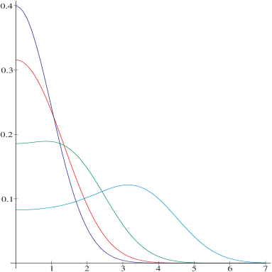
Figure 1: The probability densities that result from the deformation
$\hat{\phi}_{f}=i(a_{f}-a_{f}^{\dagger})+\alpha(f)\hat{d}_{\zeta}+\alpha^{*}(f)\hat{d}_{\zeta}^{\dagger}$, with $(f,f)=1$ and $|\alpha(f)|=0$ (blue,
highest function at zero), $\frac{1}{3}$ (red, second highest), $1$ (green, third
highest), $3$ (cyan, lowest function at zero) [colour on the web].

We can also compute characteristic functions for higher powers such as $\hat{\phi}_{f}=i(a_{f}-a_{f}^{\dagger})+\alpha(f)(\hat{d}_{\zeta}+\hat{d}_{\zeta}^{\dagger})^{k}$,

$$k=1 \longrightarrow {}_{0}F_{1}(;1;-(\lambda\alpha(f))^{2})e^{-{\frac{1}{2}}\lambda^{2}(f,f)}=J_{0}(2\lambda\alpha(f))e^{-{\frac{1}{2}}\lambda^{2}(f,f)},$$

$$k=3 \longrightarrow {}_{2}F_{3}({\scriptstyle\frac{1}{6}},{\scriptstyle\frac{5}{6}};{\scriptstyle\frac{1}{3}},{\scriptstyle\frac{2}{3}},1;-16(\lambda\alpha(f))^{2})e^{-{\frac{1}{2}}\lambda^{2}(f,f)},$$

$$k=5 \longrightarrow {}_{4}F_{5}({\scriptstyle\frac{1}{10}},{\scriptstyle\frac{3}{10}},{\scriptstyle\frac{7}{10}},{\scriptstyle\frac{9}{10}};{\scriptstyle\frac{1}{5}},{\scriptstyle\frac{2}{5}},{\scriptstyle\frac{3}{5}},{\scriptstyle\frac{4}{5}},1;-256(\lambda\alpha(f))^{2})e^{-{\frac{1}{2}}\lambda^{2}(f,f)},$$

$$\mathit{etc.},$$

$$k=0 \longrightarrow {}_{0}F_{0}(;;2i\lambda\alpha(f))e^{-{\frac{1}{2}}\lambda^{2}(f,f)}=e^{2i\lambda\alpha(f)}e^{-{\frac{1}{2}}\lambda^{2}(f,f)},$$

$$k=2 \longrightarrow {}_{1}F_{1}({\scriptstyle\frac{1}{2}};1;4i\lambda\alpha(f))e^{-{\frac{1}{2}}\lambda^{2}(f,f)}=J_{0}(2\lambda|\alpha(f)|)e^{2i\lambda\alpha(f)}e^{-{\frac{1}{2}}\lambda^{2}(f,f)},$$

$$k=4 \longrightarrow {}_{2}F_{2}({\scriptstyle\frac{1}{4}},{\scriptstyle\frac{3}{4}};{\scriptstyle\frac{1}{2}},1;16i\lambda\alpha(f))e^{-{\frac{1}{2}}\lambda^{2}(f,f)},$$

$$k=6 \longrightarrow {}_{3}F_{3}({\scriptstyle\frac{1}{6}},{\scriptstyle\frac{3}{6}},{\scriptstyle\frac{5}{6}};{\scriptstyle\frac{1}{3}},{\scriptstyle\frac{2}{3}},1;64i\lambda\alpha(f))e^{-{\frac{1}{2}}\lambda^{2}(f,f)},$$

$$\mathit{etc.}$$

The $k=0$ entry is trivially tractable, indeed trivial; otherwise only the $k=2$ entry is immediately tractable, being just a trivially displaced version of the $k=1$ entry we have just discussed, because $(d_{\zeta}+d_{\zeta}^{\dagger})^{2}=(d_{2\zeta}+d_{2\zeta}^{\dagger})+2$. The combinatorics for arbitrary Hermitian functions of $\hat{d}_{\zeta}$ and $\hat{d}_{\zeta}^{\dagger}$ added to $i(a_{f}-a_{f}^{\dagger})$, potentially using multiple Poincaré invariant displacement functions $\zeta_{i}$, can be as complicated as we care to consider.

Further possibilities that must be considered, because $\hat{d}_{\zeta}$ cannot generally be taken to be linear in $\zeta$, are fields such as $i(a_{f}-a_{f}^{\dagger})+\alpha(f)(\hat{d}_{\beta(f)\zeta}+\hat{d}_{\beta(f)\zeta}^{\dagger})$, which are distinct from the other fields considered in this section even though the vacuum state 1-measurement probability densities are independent of $\beta(f)\zeta$. If we add two displacement function components, as in $i(a_{f}-a_{f}^{\dagger})+\alpha_{1}(f)(\hat{d}_{\beta_{1}(f)\zeta}+\hat{d}_{\beta_{1}(f)\zeta}^{\dagger})+\alpha_{2}(f)(\hat{d}_{\beta_{2}(f)\zeta}+\hat{d}_{\beta_{2}(f)\zeta}^{\dagger})$ there is a complex modulation of the vacuum state 1-measurement probability density as the proportion of $\beta_{1}(f)$ to $\beta_{2}(f)$ changes.

4 Displacements of the field observable-II

The first deformation of $\hat{\phi}_{f}$ that we will discuss in this section is

$$\hat{\phi}_{f}=i(a_{f}-a_{f}^{\dagger})(\hat{d}_{\zeta}+\hat{d}_{\zeta}^{\dagger}).$$ (28)

As in the previous section, this is Hermitian and satisfies microcausality, but the algebra of observables generated by the observable field is finally different,

$$[\hat{\phi}_{f},\hat{\phi}_{g}]=[(g,f)-(f,g)](\hat{d}_{\zeta}+\hat{d}_{\zeta}^{\dagger})^{2},$$ (29)

even though the algebra satisfied by the creation and annihilation operators is unchanged. The change in the algebra of observables gives some cause to think that physics associated with this type of construction may be significantly different. $(\hat{d}_{\zeta}+\hat{d}_{\zeta}^{\dagger})^{2}$ is a central element in the algebra generated by $\hat{\phi}_{f}$.

The characteristic function of the vacuum state 1-measurement probability density is

$$\chi_{P}(\lambda|f) = \varphi_{0}(e^{i\lambda\hat{\phi}_{f}})$$ (30)

$$= \varphi_{0}\left(\sum_{j=0}^{\infty}\frac{(i\lambda)^{j}i^{j}(a_{f}-a_{f}^{\dagger})^{j}(\hat{d}_{\zeta}+\hat{d}_{\zeta}^{\dagger})^{j}}{j!}\right)$$ (31)

$$= \varphi_{0}\left(\sum_{j=0}^{\infty}\frac{\lambda^{2j}(a_{f}-a_{f}^{\dagger})^{2j}}{(2j)!}\frac{(2j)!}{j!^{2}}\right)$$ (32)

$$= \sum_{j=0}^{\infty}\frac{(-\lambda^{2}(f,f))^{j}}{(2j)!}\frac{(2j)!}{2^{j}j!}\frac{(2j)!}{j!^{2}}$$ (33)

$$= {}_{1}F_{1}({\scriptstyle\frac{1}{2}};1;-2\lambda^{2}(f,f))=I_{0}(\lambda^{2}(f,f))e^{-\lambda^{2}(f,f)},$$ (34)

where $\varphi_{0}((a_{f}-a_{f}^{\dagger})^{2j})=(-(f,f))^{j}\frac{(2j)!}{2^{j}j!}$ is a useful identity for the conventional vacuum state. $\chi_{P}(\lambda|f)$ can be inverse Fourier transformed, using [4, 7.663.2 or 7.663.6], to obtain

$$\rho_{P}(x|f)=\frac{1}{\sqrt{8\pi^{3}(f,f)}}\exp{\left(-\frac{x^{2}}{16(f,f)}\right)}K_{0}\left(\frac{x^{2}}{16(f,f)}\right).$$ (35)

This has variance $2(f,f)$, in contrast to the variance $(f,f)$ for the quantum field $i(a_{f}-a_{f}^{\dagger})$. $\rho_{P}(x|f)$ is displayed with variance $2(f,f)=2$ together with the Gaussian for $(f,f)=1$ in figure 2.

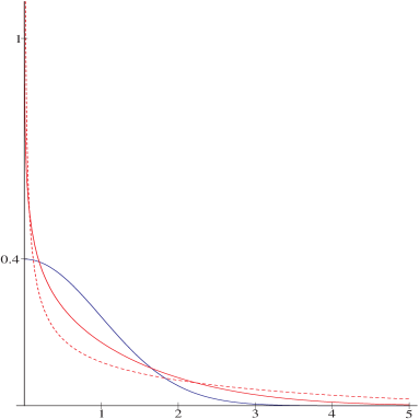
Figure 2: The probability density that results from the deformation
$\hat{\phi}_{f}=i(a_{f}-a_{f}^{\dagger})(\hat{d}_{\zeta}+\hat{d}_{\zeta}^{\dagger})$, with $(f,f)=1$, variance 2 (in red), compared with
the conventional Gaussian, with $(f,f)$, variance 1 (in blue), and the probability
density that results from the deformation $\hat{\phi}_{f}=i(a_{f}-a_{f}^{\dagger})(\hat{d}_{\zeta}+\hat{d}_{\zeta}^{\dagger})^{2}$, with
$(f,f)=1$, variance 6 (dashed, in red)[colour on the web].

The vacuum state probability density $\rho_{P}(x|f)$ is again independent of $\zeta$; it is infinite at zero, but it is also integrable enough over the real line for all finite moments to exist, which of course we computed explicitly in order to compute $\chi_{P}(\lambda|f)$.

The probability density $\rho_{P}(x|f)$ is significantly concentrated both near zero and near $\pm\infty$, relative to the conventional Gaussian probability density. If we compare with a Gaussian that has the same variance, there is a 10 times greater probability of observing a value beyond about 3.66 standard deviations, a 100 times greater probability of observing a value beyond about 4.84 standard deviations, and a 1000 times greater probability of observing a value beyond about 5.76 standard deviations. I suppose $\rho_{P}(x|f)$ will give a fairly distinctive signature in physics, which future papers will hopefully be able to make evident, and it should be clear fairly quickly whether it can be used to model events in nature.

The characteristic function of the vacuum state $n$-measurement probability density is

$$\chi_{P}(\lambda_{1},\lambda_{2},...,\lambda_{n}|f_{1},f_{2},...,f_{n})=\varphi_{0}(e^{i\sum_{j}\lambda_{j}\hat{\phi}_{f_{j}}})={}_{1}F_{1}({\scriptstyle\frac{1}{2}};1;-2\underline{\lambda}^{T}F\underline{\lambda}),$$ (36)

where, as in section 2, $F$ is the gram matrix $(f_{i},f_{j})$ and $\underline{\lambda}$ is a vector of the variables $\lambda_{i}$. For $n=2$, we can inverse Fourier transform this radially symmetric function using [4, 7.663.5], to obtain

$$\rho_{P}(x_{1},x_{2}|f_{1},f_{2})=\frac{\exp{\left(-\frac{{\underline{x}^{T}F^{-1}\underline{x}}}{8}\right)}}{\sqrt{8\pi^{3}({\underline{x}^{T}F^{-1}\underline{x}})\mathrm{det}(F)}},$$ (38)

For all $n$, we can confirm, using [4, 7.672.2] that the Fourier transform of

$$\rho_{P}(x_{1},x_{2},...,x_{n}|f_{1},f_{2},...,f_{n})=\frac{\exp{\left(-\frac{{\underline{x}^{T}F^{-1}\underline{x}}}{16}\right)}W_{\frac{n}{4}-\frac{1}{4},\frac{n}{4}-\frac{1}{4}}\left(\frac{{\underline{x}^{T}F^{-1}\underline{x}}}{8}\right)}{2^{\frac{3n}{4}-\frac{3}{4}}({\underline{x}^{T}F^{-1}\underline{x}})^{\frac{n}{4}+\frac{1}{4}}\sqrt{\pi^{n+1}\mathrm{det}(F)}}$$ (39)

is ${}_{1}F_{1}({\scriptstyle\frac{1}{2}};1;-2\underline{\lambda}^{T}F\underline{\lambda})$, where $W_{a,b}(z)$ is Whittaker’s confluent hypergeometric function. Although these mathematical derivations of probability densities can be derived, and give a distinct insight, the moments, which are essentially what are physically measurable, can be determined more easily from the characteristic functions, or directly from the action of a state on an observable.

We can also compute characteristic functions for higher powers of displacement operators, $\hat{\phi}_{f}=i(a_{f}-a_{f}^{\dagger})(\hat{d}_{\zeta}+\hat{d}_{\zeta}^{\dagger})^{k}$,

$$k=1 \longrightarrow {}_{1}F_{1}({\scriptstyle\frac{1}{2}};1;-2\lambda^{2}(f,f))=I_{0}(\lambda^{2}(f,f))e^{-\lambda^{2}(f,f)},$$

$$k=2 \longrightarrow {}_{2}F_{2}({\scriptstyle\frac{1}{4}},{\scriptstyle\frac{3}{4}};{\scriptstyle\frac{1}{2}},1;-8\lambda^{2}(f,f)),$$

$$k=3 \longrightarrow {}_{3}F_{3}({\scriptstyle\frac{1}{6}},{\scriptstyle\frac{3}{6}},{\scriptstyle\frac{5}{6}};{\scriptstyle\frac{1}{3}},{\scriptstyle\frac{2}{3}},1;-32\lambda^{2}(f,f)),$$

$$k=4 \longrightarrow {}_{4}F_{4}({\scriptstyle\frac{1}{8}},{\scriptstyle\frac{3}{8}},{\scriptstyle\frac{5}{8}},{\scriptstyle\frac{7}{8}};{\scriptstyle\frac{1}{4}},{\scriptstyle\frac{2}{4}},{\scriptstyle\frac{3}{4}},1;-128\lambda^{2}(f,f)),$$

$$\mathit{etc.,}$$

which in general have Meijer’s $G$-functions as inverse Fourier transforms [4, 7.542.5]. For $k=2$, again using [4, 7.672.2], with different substitutions, we can derive the probability density

$$\rho_{P2}(x|f)=\frac{1}{\sqrt{64\pi^{3}(f,f)}}\exp{\left(-\frac{x^{2}}{64(f,f)}\right)}K_{\frac{1}{4}}\left(\frac{x^{2}}{64(f,f)}\right),$$ (40)

This has variance $6(f,f)$; it is plotted for $(f,f)=1$ in Figure 2. In general we can multiply $i(a_{f}-a_{f}^{\dagger})$ by any self-adjoint polynomial in $\hat{d}_{\beta(f)\zeta}$ and $\hat{d}_{\beta(f)\zeta}^{\dagger}$. It will be interesting to discover what range of probability densities this will allow us to construct.

5 Discussion

This mathematics is essentially quite clear and simple, but it is also rather rich and nontrivial, and there are lots of concrete models. It will be apparent that I do not have proper control of the full range of possibilities. From philosophical points of view that seek a uniquely preferred model and that find the tight constraints of renormalization on acceptable physical models congenial, it will be seen as problematic that there is a plethora of models, but a loosening of constraints accords well with our experience of wide diversity in the natural world, and is no more than a return to the almost unconstrained diversity of classical particle and field models.

It is so far rather unclear how to understand the mathematics as physics, but any interpretation will follow a common (but not universal) quantum field theoretical assumption that we measure probabilities and correlation functions of scalar observables that are indexed by test functions. There are existing ways of discussing condensed matter physics that are fairly amenable to this style of interpretation, but it is likely that we will have to abandon some of our existing ways of talking about particles to accommodate this mathematics.

It is also reiterated here, following [1], that the positive spectrum condition on the energy, which has been so much part of the quantum field theoretical landscape, should be deprecated, because energy (and as well energy density) is unobservable, infinite, and nonlocal. If we think of the random field that is the classical equivalent of a given quantum field, taking $[a_{f},a_{g}^{\dagger}]=(g,f)+(f,g)$ so that the commutator is real and $[\hat{\phi}_{f},\hat{\phi}_{g}]=0$ for all test functions, it is clear that we are discussing an essentially fractal structure, for which differentiation and energy density at a point are undefined. From a proper mathematical perspective, we should consider only finite local observables. We have accepted renormalization formalisms that manage infinities only in lack of a finite alternative, a basis for which this paper and its precursor provide.

The method of section 4 is perhaps more significant mathematically than the methods of sections 2 and 3, insofar as the quantum field observables of section 4 satisfy modified commutation relations, in common with the methods for constructing nonlinear quantum fields that are presented in [1]. However, quantum theory somewhat exaggerates the importance of commutation relations between quantum mechanically ideal measurement devices — the trivial commutation relations of classically ideal measurement devices can give a description of experiments that is equally empirically adequate[5, 6], and ideal measurement devices between the quantum and the classical can also be used as points of reference[7].

Physics emphasizes a commitment to observed statistics, which present essentially uncontroversial lists of numbers, but it is far more difficult to describe what we believe we have measured than the statistics and the lists of numbers themselves. It might be said, for example, that “we have measured the momentum of a particle”, and cite a list of times and places where devices triggered, ignoring the delicate questions of (1) whether there is any such thing as “a particle”, (2) whether a particle can be said to have any well-defined properties at all, and (3) whether particles have “momentum” in particular. It makes sense to describe a measurement in such a way, because it forms a significant part of a coordinatization of the measurement that is good enough for the experiment and its results to be reproduced, but an alternative conceptualization can have a radical effect on our understanding.

References

[1]
Morgan P 2006, quant-ph/0512190.
[2]
Katriel J and Quesne C 1996, J. Math. Phys. 37 1650.
[3]
Haag R 1996, Local Quantum Physics, 2nd Edition (Springer-Verlag: Berlin).
[4]
Gradshteyn I S and Ryzhik I M 2000, Table of Integrals, Series, and Products,
6th Edition (Academic Press: San Diego).
[5]
Morgan P (to appear), Proceedings of the Conference on the Foundations of
Probability and Physics-4, Växjö, 2006
(American Institute of Physics: College Park, MD);
quant-ph/0607165.