From Objective Amplitudes to Bayesian Probabilities

Abstract

We review the Consistent Amplitude approach to Quantum Theory and argue that quantum probabilities are explicitly Bayesian. In this approach amplitudes are tools for inference. They codify objective information about how complicated experimental setups are put together from simpler ones. Thus, probabilities may be partially subjective but the amplitudes are not.

1 Introduction

Whether Bayesian probabilities – degrees of belief – are (1) subjective or (2) objective or (3) somewhere in between, is still a matter of controversy. I vote for (3). Probabilities will always retain a “subjective” element because translating information into probabilities involves judgments and different people will inevitably judge differently. On the other hand, not all probability assignments are equally useful and it is plausible that what makes some assignments better than others is that they represent or reflect some objective feature of the world. One might even say that what makes them better is that they are closer to the “truth”. Thus, probabilities can be characterized by both subjective and objective elements and, ultimately, it is their objectivity that makes probabilities useful.

Quantum mechanics adds an interesting twist because the recipe for calculating quantum probabilities is inflexible: apply Born’s rule to the amplitudes. There seems to be no room for judgments here. One possibility is that the objective nature of the wave function extends also to the quantum probabilities. In this view quantum and Bayesian probabilities differ in an essential way: quantum probabilities are not Bayesian. A second possibility is that it is the other way around and it is the subjectivity of the probabilities that infects the wave functions. The purpose of this paper is to argue for a third possibility.

Our goal here is to review the main ideas behind the Consistent Amplitude approach to Quantum Theory (CAQT) [1]-[3] in order to argue that there is no need to distinguish between quantum and classical probabilities. In the CAQT approach probabilities are explicitly Bayesian – they reflect the degree to which we believe that detectors will successfully detect – and yet, there is nothing subjective about the wave function that conveys the relevant information about the (idealized) experimental setup. The situation here is quite analogous to assigning Bayesian probabilities to the outcomes of a die toss based on the objective information that the (idealized) die is a perfectly symmetric cube. The probabilities may be partially subjective, but the information on which they are based is intended to represent an objective feature of the world.

Many discussions on the foundations of quantum theory start from the abstract mathematical formalism of Hilbert spaces and some postulates or rules prescribing how the formalism should be used. Their goal is to discover a suitable interpretation. The CAQT is different in that it proceeds in the opposite direction: first one specifies the objective the theory is meant to accomplish and then a suitable formalism is derived from a set of “reasonable” assumptions. In a sense, the interpretation is the starting point and the formalism is derived from it.

The objective of the CAQT is to predict the outcomes of certain idealized experiments on the basis of information about how complicated experimental setups are put together from simpler ones. The theory is, by design, a theory of inference from available information. The “reasonable” assumptions are four. The first specifies the kind of setups about which we want to make predictions. The second assumption establishes what is the relevant information on the basis of which the predictions will be made and how this information is codified. It is at this stage that amplitudes and wave functions are introduced as tools for the consistent manipulation of information. The third and fourth assumptions provide the link between the amplitudes and the actual prediction of experimental outcomes. Although none of these assumptions refer to probabilities, all the elements of quantum theory, including indeterminism and the Born rule, Hilbert spaces, linear and unitary time evolution, are derived. [1]-[3]

2 Setups and amplitudes

The first and most crucial step is a decision about the subject matter. We choose a pragmatic, operational approach: the objective of quantum theory is to predict the outcomes of experiments carried out with certain idealized setups.

Next we note that if setups are related in some way – perhaps two setups can be connected to build a third one – then information about one may be relevant to predictions about the other. This suggests that one should identify the possible relations among setups. To avoid irrelevant technical distractions we consider a very simple quantum system, a “particle” that lives on a discrete lattice and has no spin or other internal structure. (In fact, whether the system is a particle or a wave or both or neither is immaterial; the word ‘particle’ is selected only because a word, some word, must be used to refer to the system.) The generalization to more complex configuration spaces should be straightforward.

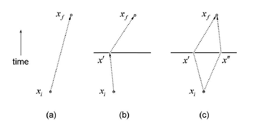
Figure 1: (a) The simplest setup $[x_{f},x_{i}]$. (b) Two successive setups $[x_{f},x^{\prime}]$ and $[x^{\prime},x_{i}]$ are combined with the and operation. (c) Two setups in parallel, $[x_{f},x^{\prime},x_{i}]$ and $[x_{f},x^{\prime\prime},x_{i}]$ are combined with the or operation.

The simplest experimental setup, denoted by $[x_{f},x_{i}]$, is shown in Fig. 1(a). It consists of a source at the space-time point $x_{i}=(\vec{x}_{i},t_{i})$ and a detector at $x_{f}=(\vec{x}_{f},t_{f})$. Both $\vec{x}_{i}$ and $\vec{x}_{f}$ are assumed to be points on a discrete lattice and the intermediate region may be filled by various kinds of fields. In Fig. 1(b) we show a slightly more complex setup that we denote by $[x_{f},x^{\prime},x_{i}]$ where the source is at $x_{i}$, the detector at $x_{f}$, and we have introduced a “filter” that blocks all paths from $x_{i}$ to $x_{f}$ except via the intermediate point $x^{\prime}$. The possibility of introducing many filters each with several holes (as in Fig. 1c) leads to allowed setups of the general form $a=[x_{f},s_{n},s_{n-1},\ldots,s_{2},s_{1},x_{i}]$ where each $s_{n}=(x_{n},x_{n}^{\prime},x_{n}^{\prime\prime},\ldots)$ represents a filter at time $t_{n}$, intermediate between $t_{i}$ and $t_{f}$, with multiple holes at $\vec{x}_{n},\vec{x}_{n}^{\prime},\vec{x}_{n}^{\prime\prime},\ldots$

There are two basic kinds of relations among setups. The first, called and, arises when two setups $a$ and $b$ are placed in immediate succession resulting in a third setup which we denote by $ab$. It is necessary that the destination point of the earlier setup coincide with the source point of the later one, otherwise the combined $ab$ is not allowed. For example, $[x_{f},x^{\prime}][x^{\prime},x_{i}]=[x_{f},x^{\prime},x_{i}]$ is shown in Fig. 1(b). With the single setup $[x_{f},x^{\prime},x_{i}]$ we can perform several different experiments. We can place a source at $x_{i}$ and the detector at $x^{\prime}$ in which case we are only using the $[x^{\prime},x_{i}]$ component; or we can place the source at $x^{\prime}$ and the detector at $x_{f}$ and use only the $[x_{f},x^{\prime}]$ component; or we can place a source at $x_{i}$, the detector at $x_{f}$, and use the whole thing $[x_{f},x^{\prime},x_{i}]$. Although we can only do one of these experiments at a time, the three experiments are clearly related and knowing something about one setup may be helpful in making predictions about another.

The second relation, called or, arises from the possibility of opening additional holes in any given filter. Specifically, when (and only when) two setups $a^{\prime}$ and $a^{\prime\prime}$ are identical except on one single filter where none of the holes of $a^{\prime}$ overlap any of the holes of $a^{\prime\prime}$, then we may form a third setup $a$, denoted by $a^{\prime}\vee a^{\prime\prime}$, which includes the holes of both $a^{\prime}$ and $a^{\prime\prime}$. The example

$$[x_{f},(x^{\prime},x^{\prime\prime}),x_{i}] =[x_{f},x^{\prime},x_{i}]\vee[x_{f},x^{\prime\prime},x_{i}]$$ (1)

$$=([x_{f},x^{\prime}][x^{\prime},x_{i}])\vee([x_{f},x^{\prime\prime}][x^{\prime\prime},x_{i}])$$ (2)

is shown in Fig. 1(c). Again we see that we can perform a wide variety of related experiments with the same setup by judicious placement of source and detector and by blocking or not the appropriate holes.

Provided the relevant setups are allowed the basic properties of and and or are quite obvious: or is commutative, but and is not; both and and or are associative, and finally, and distributes over or but not vice-versa. One should emphasize that these are physical rather than logical connectives. They represent our idealized ability to construct more complex setups out of simpler ones and they differ substantially from their Boolean and quantum logic counterparts. In Boolean logic not only and distributes over or but or also distributes over and, while in quantum logic propositions refer to quantum properties at one time rather than to processes in time.

Thus, our first assumption is

• The goal of quantum theory is to predict the outcomes of experiments involving setups built from components connected through and and or.

Having identified relations among setups we now seek a way to handle them quantitatively. A representation of and/or can be obtained by assigning a complex number $\phi(a)$ to each setup $a$ in such a way that relations among setups translate into relations among the corresponding complex numbers. What gives the theory its robustness, its uniqueness, is the requirement that the assignment be consistent: if there are two different ways to compute $\phi(a)$ the two answers must agree. The remarkable consequence of requiring consistency is embodied in the following

Regraduation Theorem: Given one consistent representation of and/or in terms of complex numbers $\phi(a)$, one can “regraduate” with an appropriately chosen function $\psi$ to obtain an equivalent and more convenient assignment, $\psi(a)=\psi(\phi(a))$, so that and and or are respectively represented by multiplication and addition,

$$\psi\left(ab\right)=\psi\left(a\right)\psi\left(b\right)\quad\text{and\quad}\psi\left(a\vee a^{\prime}\right)=\psi\left(a\right)+\psi\left(a^{\prime}\right)\text{.}$$ (3)

Complex numbers assigned in this way will be called amplitudes. The theorem is proved in [1, 2]. (For an independent earlier derivation see ref. [5].)

It would be interesting to explore the consequences of keeping track of more information about the setups by using representations of and/or in terms of more complicated mathematical objects. It is likely that the resulting theory would differ from quantum mechanics in important ways. For our current purposes however we restrict ourselves to a representation in terms of amplitudes. This is our second assumption,

• The relevant information for predicting the outcome of an experiment with a setup $a$ is codified into its complex amplitude $\psi(a)$.

3 Wave functions and time evolution

The observation, already expressed by Feynman [6], that leads to the fundamental evolution equation (and eventually to path integrals) is that a filter that is totally covered with holes is equivalent to having no filter at all,

$$[x_{f},x_{i}]=\bigvee_{\text{all}\,\,\vec{x}\,\text{at}\,t}([x_{f},x_{t}][x_{t},x_{i}])~{}.$$ (4)

In terms of the corresponding amplitudes, this is quantitatively expressed as

$$\psi(x_{f},x_{i})=\sum_{\text{all}\,\vec{x}\,\text{at}\,t}\psi(x_{f},x_{t})\,\psi(x_{t},x_{i}).$$ (5)

Since we are interested only in the response of the detectors we find that in there are situations where amplitudes keep track of too much information. Indeed, note that there are many possible combinations of starting points $x_{i}$ and of interactions prior to the time $t$ that will result in identical evolution after time $t$. What these different possibilities have in common is that they all lead to the same numerical value for the amplitude $\psi(x_{t},x_{i})$. It is therefore convenient to set $\Psi(\vec{x},t)=\psi(x_{t},x_{i})$ and omit all reference to the irrelevant starting point $x_{i}$. The object thus introduced, $\Psi(\vec{x},t)$, is called a wave function. The usual language is that $\Psi(\vec{x},t)$ describes the state of the particle at time $t$. In the CAQT approach we say that $\Psi(\vec{x},t)$ encodes information about those features of the setup prior to $t$ that are relevant to time evolution after $t$.

The evolution equation can then be written as

$$\Psi(\vec{x}_{f},t_{f})=\sum_{\text{all }\,\vec{x}\,\text{at}\,t}\psi(\vec{x}_{f},t_{f};\vec{x},t)\,\Psi(\vec{x},t)\text{,}$$ (6)

which is equivalent to a linear Schrödinger equation as can easily be seen [1][2] by differentiating with respect to $t_{f}$ and evaluating at $t_{f}=t$. Thus, a quantum theory formulated in terms of consistently assigned amplitudes must be linear: nonlinear modifications of quantum mechanics must either violate assumptions A1 or A2 or else be internally inconsistent.

4 Hilbert space

In the usual approach to quantum theory the linearity embodied in the principle of superposition and the linearity of the Schrodinger equation seem completely unrelated. Indeed, all proposals for a non-linear quantum mechanics have invariably maintained the former and broken the latter. Within the CAQT approach this is not allowed. One cannot preserve the linearity of superpositions and break the linearity of evolution because both follow from the same consistency requirement that led to the sum and product rules for amplitudes.

The superposition principle states that if a system can be prepared in a state $\Psi^{\prime}$ and it can be prepared in another state $\Psi^{\prime\prime}$ then it can also be prepared in a linear superposition $\Psi=\alpha\Psi^{\prime}+\beta\Psi^{\prime\prime}$. An interesting question is whether the superposition can actually be prepared. Given a generic pair of states $\Psi^{\prime}$ and $\Psi^{\prime\prime}$, what is the specific setup that will prepare the state $\alpha\Psi^{\prime}+\beta\Psi^{\prime\prime}$?

Within the CAQT approach this annoying question does not arise because we are not interested in preparing arbitrary states, but only in predicting the outcomes of experiments with those special setups described in assumption A1. For these special setups it is easy to see that linear superpositions do arise. For example, let $\Psi^{\prime}(\vec{x},t)=\psi(\vec{x},t;\vec{x}^{\prime},t_{0})$ be the wave function at time $t$ when the source is at $(\vec{x}^{\prime},t_{0})$, and let $\Psi^{\prime\prime}(\vec{x},t)=\psi(\vec{x},t;\vec{x}^{\prime\prime},t_{0})$ be the wave function when the source is at $(\vec{x}^{\prime\prime},t_{0})$. See Fig. 2. Linear superpositions of $\Psi^{\prime}(\vec{x},t)$ and $\Psi^{\prime\prime}(\vec{x},t)$ can be prepared by placing a filter at $t_{0}$ with holes at $\vec{x}^{\prime}$ and $\vec{x}^{\prime\prime}$ and a source at a point $(\vec{x}_{i},t_{i})$ prior to $t_{0}$. Then the overall amplitude for this new setup, $\psi(\vec{x},t;\vec{x}_{i},t_{i})$, is

$$\Psi(\vec{x},t)=\alpha\Psi^{\prime}(\vec{x},t)+\beta\Psi^{\prime\prime}(\vec{x},t)\text{ ,}$$ (7)

where $\alpha=\psi(\vec{x}^{\prime},t_{0};\vec{x}_{i},t_{i})$ and $\beta=\psi(\vec{x}^{\prime\prime},t_{0};\vec{x}_{i},t_{i})$. Notice that the complex numbers $\alpha$ and $\beta$ can be changed at will by moving the starting point $(\vec{x}_{i},t_{i})$ or by introducing additional fields between $t_{i}$ and $t_{0}$.

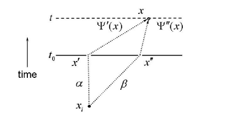
Figure 2: Illustrating how the superposition principle follows from the sum and product rules for consistent amplitudes.

Thus, as a consequence of the sum and product rules, eq.(3), linear superpositions of wave functions arise naturally and we can ask what else is needed for them to form a Hilbert space. The basic question is whether an equally compelling inner product is available. The answer is quite illuminating because of the support it gives to viewing quantum mechanics as a theory of inference rather than as a law of nature.

An inner product defines lengths and angles. We find that without any additional assumptions the basic components of setups, the filters, take us a long way toward an inner product because they already supply us with a concept of orthogonality. The action of a filter $P$ with holes at a set of points $\vec{x}_{p}$ is to turn the wave function $\Psi(\vec{x})$ into the wave function $P\Psi(\vec{x})=\sum_{p}\delta_{\vec{x},\vec{x}_{p}}\Psi(\vec{x})$. Since the filters $P$ act as projectors, $P^{2}=P$, it follows that any given filter defines two special classes of wave functions. One is the subspace of wave functions that are transmitted by the filter without any changes, and the other is the subspace of wave functions that are completely blocked. We will define these two subspaces as being orthogonal to each other.

Any wave function can be decomposed into orthogonal components, $\Psi=\Psi_{P}+\Psi_{1-P}$ where $\Psi_{P}=P\Psi$ is unaffected by the filter and $\Psi_{1-P}=(1-P)\Psi$ is blocked: $P\Psi_{P}=\Psi_{P}$ and $P\Psi_{1-P}=0$. A particularly convenient expansion in orthogonal components is that defined by a complete set of elementary filters. A filter $P_{i}$ is elementary if it has a single hole at $\vec{x}_{i}$. It acts by multiplying $\Psi(\vec{x})$ by $\delta_{\vec{x},\vec{x}_{i}}$. The set is complete if $\sum_{i}P_{i}=1$. Then $\Psi(\vec{x})=\sum_{i}A_{i}\,\delta_{\vec{x},\vec{x}_{i}}$, where $A_{i}=\Psi(\vec{x}_{i})$.

At this point it is convenient to introduce the familiar Dirac notation. Instead of $\Psi(\vec{x})$ and $\delta_{\vec{x},\vec{x}_{i}}$ we shall write $|\Psi\rangle$ and $|i\rangle$, so that $|\Psi\rangle=\sum_{i}A_{i}|i\rangle$. The question is what else, in addition to orthogonality, do we need to define the inner product. Recall that an inner product satisfies three conditions: (a) $\langle\Psi|\Psi\rangle\geqslant 0$ with $\langle\Psi|\Psi\rangle=0$ if and only if $|\Psi\rangle=0$, (b) linearity in the second factor, and (c) antilinearity in the first factor, $\langle\Phi|\Psi\rangle=\langle\Psi|\Phi\rangle^{\ast}$. Conditions (b) and (c) define the product of $|\Phi\rangle=\sum_{j}B_{j}|j\rangle$ with $|\Psi\rangle=\sum_{i}A_{i}|i\rangle$ in terms of the product of $|j\rangle$ with $|i\rangle$,

$$\langle\Phi|\Psi\rangle=\sum_{i}B_{j}^{\ast}A_{i}\langle j|i\rangle~{}.$$ (8)

The orthogonality of the basis functions $\delta_{\vec{x},\vec{x}_{i}}$ is naturally encoded into the inner product by setting $\langle j|i\rangle=0$ for $i\neq j$, but the case $i=j$ remains undetermined, constrained by condition (a) to be real and positive. Clearly an additional assumption is necessary. Here it is:

• If there is no reason to prefer one region of configuration space over another they should be assigned equal a priori weight.

We therefore choose $\langle i|i\rangle$ equal to a constant which, without losing generality, we set equal to one:

$$\langle i|j\rangle=\delta_{ij}\Rightarrow\langle\Phi|\Psi\rangle=\sum_{i}B_{i}^{\ast}A_{i},$$ (9)

and this leads to the Hilbert norm $\left\|\Psi\right\|^{2}=\langle\Psi|\Psi\rangle=\sum_{i}|A_{i}|^{2}$. The significance of A3 will be better understood once we explore its implications in the next section.

5 Probabilities: the Born rule

Finally, we get to the question of using the information encoded into amplitudes to predict the outcomes of experiments. Our argument invokes time evolution, eq. (6), in an essential way. This is in contrast to other derivations of the Born rule (such as Gleason’s) which are essentially static.

It is perhaps best to start with a simple special case. Suppose that the preparation procedure is such that $\Psi(\vec{x},t)$ vanishes at a certain point $(\vec{x}_{0},t)$. Then, according to eq. (6), placing an obstacle at the single point $(\vec{x}_{0},t)$ (i.e., placing a filter at $t$ with holes everywhere except at $\vec{x}_{0}$) has no effect on the subsequent evolution of $\Psi$. Since the mathematical relations among amplitudes are meant to reflect the corresponding physical relations among setups, it seems natural to assume that the presence or absence of the obstacle at $\vec{x}_{0}$ will have no observable effects. What if the obstacle was itself a detector? It is just as natural to assume that since the obstacle/detector inflicts no action on the system, then it must not itself suffer any reaction. Therefore, we conclude that when $\Psi(\vec{x}_{0},t)=0$ the particle will not be detected at $(\vec{x}_{0},t)$.

Convincing and natural as this argument might be, it is important to recognize that an assumption was made: no amount of logic could conceivably bridge the gap from a mathematical representation in terms of amplitudes to the prediction of an actual physical event. The assumption can be generalized to the following general interpretative rule:

• If the introduction at time $t$ of a filter blocking those components of the wave function characterized by a certain property $\mathcal{P}$ has no effect on the future evolution of a particular wave function $\Psi(t)$ then when the wave function happens to be $\Psi\left(t\right)$ the property $\mathcal{P}$ will not be detected.

Note that A4 deals with a situation of complete certainty; no probabilities are mentioned.

The deduction of the Born rule now proceeds as in ref. [2]. Briefly the idea is as follows. We want to predict the outcome of an experiment in which a detector is placed at a certain $\vec{x}_{k}$ when the system is in state $|\Psi\rangle=\sum_{i}A_{i}|i\rangle$. In [2] we showed that the state for an ensemble of $N$ identically prepared, independent replicas of our particle is the product $|\Psi_{N}\rangle=\prod_{\alpha=1}^{N}|\Psi_{\alpha}\rangle$. Now we apply the interpretative rule A4. Suppose that in the $N$-particle configuration space we place a special filter, denoted by $P_{f,\varepsilon}^{k}$, the action of which is to block all components of $|\Psi_{N}\rangle$ except those for which the fraction $n/N$ of replicas at $\vec{x}_{k}$ lies in the range from $f-\varepsilon$ to $f+\varepsilon$. The difference between the states $P_{f,\varepsilon}^{k}|\Psi_{N}\rangle$ and $|\Psi_{N}\rangle$ is measured by the relative Hilbert distance, $||P_{f,\varepsilon}^{k}|\Psi_{N}\rangle-|\Psi_{N}\rangle||^{2}/\langle\Psi_{N}|\Psi_{N}\rangle$. The result of this calculation is [2]

$$\underset{N\rightarrow\infty}{\lim}\,\left\|P_{f,\varepsilon}^{k}|\Psi_{N}\rangle-|\Psi_{N}\rangle\right\|^{2}=1-\int_{f-\varepsilon}^{f+\varepsilon}\delta\left(f^{\prime}-|A_{k}|^{2}\right)df^{\prime}\text{ ,}$$ (10)

where we have normalized $\langle\Psi|\Psi\rangle=\langle\Psi_{N}|\Psi_{N}\rangle=1$.

We see that for large $N$ the filter $P_{f,\varepsilon}^{k}$ has no effect on the state $|\Psi_{N}\rangle$ provided $f$ lies in a range $2\varepsilon$ about $|A_{k}|^{2}$. Therefore, according to A4, the state $|\Psi_{N}\rangle$ does not contain any fractions outside this range. On choosing stricter filters with $\varepsilon\rightarrow 0$ we conclude that we can predict with complete certainty that detection at $\vec{x}_{k}$ will occur for a fraction $|A_{k}|^{2}$ of the replicas and that detection will not occur for the remaining fraction $1-|A_{k}|^{2}$. For any one of the identical individual replicas there is no such certainty; the best one can do is to say that detection will occur with a certain probability $\Pr(k)$. In order to be consistent with the law of large numbers the assigned value must agree with the Born rule

$$\Pr(k)=|A_{k}|^{2}\,.$$ (11)

The important role played by the inner product, introduced through assumption A3, into eq.(10) must be emphasized. In fact, had we weighted the $|i\rangle$’s differently and chosen a different normalization, say $\langle i|i\rangle=w_{i}$, the resulting probability would have been $\Pr(i)$ $=w_{i}|A_{i}|^{2}$ instead of eq.(11).

It is instructive to explore this issue further. Nothing in our choice of a discrete lattice requires it to be uniform and periodic. Indeed, a non-uniform discrete lattice could have been defined in terms of an arbitrary frame of curvilinear coordinates. If the underlying configuration space is Euclidean the use of curvilinear rather than cartesian coordinates is a matter of choice but in the general case of curved spaces curvilinear coordinates are unavoidable.

Assumption A3 suggests that each cell $i$ in the non-uniform lattice be weighted by its own volume which we will denote by $w_{i}=g_{i}^{1/2}\Delta x$. (The usual notation for a volume element in arbitrary coordinates is $g^{1/2}(x)dx$ where $g(x)$ is the determinant of the metric tensor, and $dx=dx^{1}\ldots dx^{3}$ in three dimensions.) In the continuum limit [3] we let $\Delta x\rightarrow dx$. Replacing $w_{i}^{-1}|i\rangle=(g_{i}^{1/2}\Delta x)^{-1}|i\rangle$ by$\,|\vec{x}\rangle$ the completeness condition $1=\sum_{i}P_{i}=\sum_{i}w_{i}^{-1}|i\rangle\langle i|$ becomes $1=\int g^{1/2}dx\,|\vec{x}\rangle\langle\vec{x}|$. Next, replace $\delta_{ij}/\Delta x$ by $\delta(\vec{x}-\vec{x}^{\prime})$ and the inner product $\langle i|j\rangle=w_{i}\delta_{ij}$ becomes $\langle\vec{x}|\vec{x}^{\prime}\rangle=g^{-1/2}\delta(\vec{x}-\vec{x}^{\prime})$. Finally, replace $A_{i}$ by $A(\vec{x})$ and the state $|\Psi\rangle=\sum_{i}A_{i}|i\rangle$ becomes $|\Psi\rangle=\int g^{1/2}dx\,A(\vec{x})\,|\vec{x}\rangle$. The Born rule, eq. (11), becomes

$$\Pr(dx)=g^{1/2}dx\,|A(\vec{x})|^{2}$$ (12)

which shows that $|A(\vec{x})|^{2}$ is the probability density.

It is sometimes argued that while there is an element of subjectivity in the nature of classical probabilities but that quantum probabilities are different, that they are totally objective because they are given by $|A|^{2}$. We have just shown that this assignment is neither more nor less subjective than say, assigning probabilities to each face of a die. Just like we assign probability $1/6$ when we have no reason to prefer one face of the die over another, the Born rule follows, even in curved spaces, when we have no reason to prefer one volume element over another — provided their volumes are equal.

6 Conclusion

Probabilities may be subjective but the information on the basis of which we update probabilities is not supposed to be. Indeed, we want to update from a prior to a posterior distribution because we believe the posterior distribution will give us a better assessment of truth. Posterior distributions are “objectively” better than prior distributions.

We have argued that amplitudes and wave functions codify objective information about the way experimental setups are put together. Quantum probabilities take this information into account and thereby incorporate an objective element – this is why they work. On the other hand, although amplitudes and wave functions may be representations of objective information, an element of subjectivity is introduced into the corresponding state vectors and the Hilbert space through the specification of the inner product. It was necessary to make an assumption – a judgement – about the a priori weight assigned to any region of configuration space.

It is possible to develop the CAQT approach further and use an entropic argument [3] to show that time evolution is not merely linear but that it is also unitary. This allows us to introduce observables other than position. It is also possible to consider more complex many-particle sources and detectors and thus generalize to many-particle systems. But these developments lie beyond the limited goal of this paper which was to review the argument from the objective information embodied in consistent amplitudes to the Bayesian probabilities of quantum theory.

References

- [1] A. Caticha, Phys. Lett. A244, 13 (1998) (quant-ph/9803086).
- [2] A. Caticha, Phys. Rev. A57, 1572 (1998) (quant-ph/9804012).
- [3] A. Caticha, Found. Phys. 30, 227 (2000) (quant-ph/9810074).
- [4] A. Caticha and A. Giffin, “Updating Probabilities” (physics/0608185).
- [5] Y. Tikochinsky, Int. J. Theor. Phys. 27, 543 (1988) and J. Math. Phys. 29,398 (1988); Y. Tikochinksy and S. F. Gull, J. Phys. A: Math. Gen. 33, 5615 (2000).
- [6] R. P. Feynman, Rev. Mod. Phys. 20, 267 (1948); R. P. Feynman and A. R. Hibbs, “Quantum Mechanics and Path Integrals” (McGraw-Hill, 1965).