Effective Quantum Dynamics of Interacting Systems with Inhomogeneous Coupling

Abstract

We study the quantum dynamics of a single mode/particle interacting inhomogeneously with a large number of particles and introduce an effective approach to find the accessible Hilbert space where the dynamics takes place. Two relevant examples are given: the inhomogeneous Tavis-Cummings model (e.g., $N$ atomic qubits coupled to a single cavity mode, or to a motional mode in trapped ions) and the inhomogeneous coupling of an electron spin to $N$ nuclear spins in a quantum dot.

I INTRODUCTION

In quantum optics and condensed matter physics, a great effort has been oriented to the study of single quantum systems, or a few of them, and their experimental coherent control. This is the case of cavity QED reviewcavityQED , trapped ions reviewions , quantum dots Cerletti , circuit QED Blais , among others. On the other hand, many-particle physics describes a variety of systems where collective effects may play a central role.

The interaction of a single atom with a quantized electromagnetic mode, described by the Jaynes-Cummings (JC) model JaynesCummings , has played a central role in quantum optics and other related physical systems. Among its many fundamental predictions, we can mention vacuum-field Rabi Oscillations, collapses and revivals of atomic populations, and squeezing of the radiation field review1 . Atomic cloud physics can be conveniently described by the Dicke model dicke1 , when considering the interaction of atoms with light in free space, or by the Tavis-Cummings (TC) model tavis1 , when the coupling takes place inside a cavity. In most treatments and applications of the TC model, a constant coupling between the atoms and the radiation field is assumed, simplification that greatly reduces the complexity of an analytical description cooperativeeffects ; jc1 ; jc2 ; Retzker . Even in the case of many atoms, the homogeneous-coupling case profits from the $SU(2)$ group structure of the collective operators, allowing at least numerical solutions. However, the situation is drastically different when we consider the more realistic case of inhomogeneous coupling. In this case, there is no such straightforward way to access the Hilbert space, because all angular momenta representations are mixed through the dynamical evolution of the system and no analytical approach is known.

On the other hand, electron and nuclear spin dynamics in semiconductor nanostructures has become of central interest in last years Cerletti ; Wolf , and several techniques for quantum information processing have been proposed Loss1 ; Taylor2 ; Privman ; Kane ; Levy ; Ladd . For example, ensembles of polarized nuclear spins in quantum dots Taylor and quantum Hall semiconductor nanostructures Mani have been proposed as a long-lived quantum memory for the electron spin. Recently, polarization procedures for the nuclear spins in a quantum dot have been studied theoretically zoller ; Christ06 ; DengHu , and first experiments have achieved considerable dynamical nuclear polarization Lei . However, difficulties in producing a fully polarized nuclear state suggest the necessity of analyzing the effect of imperfect polarization. This treatment faces the same theoretical challenges as the study of the inhomogeneous TC model, because of the unavoidable inhomogeneous coupling of electron and nuclear spins in quantum dots.

In this work, we develop an effective approach to study the dynamics of a single mode/particle coupled inhomogeneously to a large number of particles. In particular, we analyze in Sec. II the general interaction of a collection of two-level atoms with a quantized field mode, that is, the inhomogeneous TC model. We identify a subset of the Hilbert space that is relevant for the dynamics and show that we are able to reproduce accurate results with a small number of states. In Sec. III we consider the hyperfine interaction of a single excess electron spin confined in a quantum dot with quasi-polarized nuclear spins. Using the formalism developed in section II, we study the transfer of quantum information between those systems in the presence of a single excitation in the nuclear spin system prior to the write-in procedure. In Sec. IV, we present our concluding remarks.

II INHOMOGENEOUS TAVIS-CUMMINGS MODEL

The Hamiltonian describing the inhomogeneous coupling of $N$ atoms with a quantized single field mode, in the interaction picture and under resonant conditions, can be written as

$$\hat{H}_{\mathrm{ITC}}=\sum_{i=1}^{N}g_{i}\left(\hat{\sigma}_{i}^{-}\hat{a}^{\dagger}+\hat{\sigma}_{i}^{+}\hat{a}\right).$$ (1)

Here, $g_{i}=g({\vec{r}}_{i})$ is the (real) inhomogeneous coupling strength of atom $i$ at position ${\vec{r}}_{i}$, $\hat{\sigma}_{i}^{-}$ ($\hat{\sigma}_{i}^{+}$) is the lowering (raising) operator of atom $i$, and $\hat{a}$ ($\hat{a}^{\dagger}$) is the annihilation (creation) operator of the field mode. We will refer to this model as the inhomogeneous Tavis-Cummings (ITC) model. In the homogeneous case, $g_{i}=g$, $\forall i$, one can define as angular momentum operator $\hat{J}^{+}\propto g\sum_{i=1}^{N}\hat{\sigma}_{i}^{+}$, describing transitions between the common eigenvectors of $\hat{J}_{z}$ and $\hat{J}^{2}$, where $\hat{J}_{z}=\sum_{i=1}^{N}\hat{\sigma}_{z_{i}}$. This is not true for the inhomogeneous case, because ${\hat{\tilde{J}}^{+}}=\sum_{i=1}^{N}g_{i}\hat{\sigma}_{i}^{+}$ does not satisfy anymore the $SU(2)$ algebra. However, we will show that this problem can still be addressed with certain restrictions. The strategy consists in following the Hilbert space that the system will visit along its evolution, and implementing a truncation that will depend on the window evolution time.

Let us first consider the initial condition given by

$$|\Psi(0)\rangle=\sum_{n=0}c_{n}|n\rangle|\mathbf{\bar{0}\rangle},$$ (2)

where $|n\rangle$ denotes a photonic Fock state and $|\mathbf{\bar{0}\rangle}$ the collection of $N$ atoms in the ground state. For each product state $|n\rangle|\mathbf{\bar{0}\rangle}$, we have a fixed number of excitations, which, even in the inhomogeneous case, is conserved by the dynamics determined by $\hat{H}_{\mathrm{ITC}}$. If the initial state is $|0\rangle|\mathbf{\bar{0}\rangle}$, the unitary evolution is trivial

$$|0\rangle|\mathbf{\bar{0}\rangle\longrightarrow}|0\rangle|\mathbf{\bar{0}\rangle}.$$ (3)

Starting from initial state $|1\rangle|\mathbf{\bar{0}\rangle}$, $\hat{H}_{\mathrm{ITC}}$ produces a nontrivial dynamics via the term $\hat{\tilde{J}}^{+}\hat{a}$, so that

$$\hat{\tilde{J}}^{+}\hat{a}|1\rangle|\mathbf{\bar{0}\rangle=}|0\rangle\sum_{i=1}^{N}g_{i}|\mathbf{\bar{1}}_{i}\mathbf{\rangle},$$ (4)

where $|\mathbf{\bar{1}}_{i}\mathbf{\rangle}=\hat{\sigma}_{i}^{+}|\mathbf{\bar{0}}\rangle$ represents a $N$-atom state with one excitation in the $i$th atom. We define

$$|\mathbf{\bar{1}\rangle=}\frac{1}{\sqrt{\sum_{i=1}^{N}g_{i}^{2}}}\sum_{i=1}^{N}g_{i}|\mathbf{\bar{1}}_{i}\mathbf{\rangle},$$ (5)

a normalized state such that

$$\langle 0|\langle\mathbf{\bar{1}}|H_{\rm ITC}|1\rangle|\mathbf{\bar{0}\rangle=}\sqrt{\sum_{i=1}^{N}g_{i}^{2}}\equiv N_{0}.$$ (6)

Note that the system evolves in a closed two-dimensional subspace $\{|1\rangle|\mathbf{\bar{0}\rangle,}$ $|0\rangle|\mathbf{\bar{1}\rangle}\}$ in which all states have the same fixed number of excitations.

If we start the dynamics with the 2-excitation state $|2\rangle|\mathbf{\bar{0}\rangle}$, it evolves through

$$\hat{\tilde{J}}^{+}\hat{a}|2\rangle|\mathbf{\bar{0}\rangle} \mathbf{=} \sqrt{2}|1\rangle\sum_{i=0}g_{i}|\mathbf{\bar{1}}_{i}\mathbf{\rangle}$$ (7)

$$= \sqrt{2}N_{0}|1\rangle|\mathbf{\bar{1}\rangle}.$$

The generated state $|1\rangle|\mathbf{\bar{1}\rangle}$ produces now

$$\hat{\tilde{J}}^{+}\hat{a}|1\rangle|\mathbf{\bar{1}\rangle} \mathbf{=} \frac{1}{N_{0}}|0\rangle\sum_{i=1}^{N}g_{i}\hat{\sigma}_{i}^{+}\sum_{j=1}^{N}g_{j}|\mathbf{\bar{1}}_{j}\mathbf{\rangle}$$ (8)

$$= \frac{N_{1}}{N_{0}}|0\rangle|\mathbf{\bar{2}\rangle},$$

where

$$|\mathbf{\bar{2}\rangle}\mathbf{=}\frac{2}{N_{1}}\sum_{i<j}g_{i}g_{j}|\mathbf{\bar{2}}_{ij}\mathbf{\rangle},$$ (9)

and

$$N_{1}=\sqrt{4\sum_{i<j}g_{i}^{2}g_{j}^{2}}.$$ (10)

At the same time

$$\hat{\tilde{J}}^{-}\hat{a}^{\dagger}|1\rangle|\mathbf{\bar{1}\rangle}\mathbf{=}\sqrt{2}N_{0}|2\rangle||\mathbf{\bar{0}}\rangle.$$ (11)

On the other hand, the state $|0\rangle|\mathbf{\bar{2}\rangle}$ evolves according to

$$\hat{\tilde{J}}^{-}\hat{a}^{\dagger}|0\rangle|\mathbf{\bar{2}\rangle} \mathbf{=} |1\rangle\frac{2}{N_{1}}\sum_{k}\sum_{i<j}g_{k}g_{i}g_{j}\hat{\sigma}^{-}_{k}|\mathbf{\bar{2}}_{ij}\mathbf{\rangle}$$ (12)

$$= |1\rangle|\phi_{1}\rangle,$$

with

$$|\phi_{1}\rangle=\sum_{i}(\sum_{j\neq i}c_{ij}g_{j})|\mathbf{\bar{1}}_{i}\mathbf{\rangle},$$ (13)

and $c_{ij}=2g_{i}g_{j}/N_{1}$. The result is a one excitation state in the atomic system which is different from $|\mathbf{\bar{1}\rangle}$ defined in Eq. (5). The resulting state can be expressed  as a linear combination of $|\mathbf{\bar{1}\rangle}$ and an orthogonal state $|\mathbf{\bar{1}}_{p}\rangle$ that can be conveniently expressed as

$$|\mathbf{\bar{1}}_{p}\mathbf{\rangle=}\frac{1}{\sqrt{\langle\phi_{1}|\phi_{1}\rangle-|\langle\mathbf{\bar{1}}|\phi_{1}\mathbf{\rangle|}^{2}}}\mathbf{(}|\phi_{1}\rangle-\langle\mathbf{\bar{1}}|\phi_{1}\mathbf{\ \rangle}|\mathbf{\bar{1}\rangle)},$$ (14)

yielding

$$|1\rangle|\phi_{1}\rangle=\langle\mathbf{\bar{1}}|\phi_{1}\mathbf{\ \rangle}|1\rangle|\mathbf{\bar{1}\rangle+}\sqrt{\langle\phi_{1}|\phi_{1}\rangle-|\langle\mathbf{\bar{1}}|\phi_{1}\mathbf{\rangle|}^{2}}|1\rangle|\mathbf{\bar{1}}_{p}\mathbf{\rangle}.$$ (15)

The state $|1\rangle|\mathbf{\bar{1}}_{p}\mathbf{\rangle}$ is a new orthogonal state of the considered $2$-excitation Hilbert subspace. Via $\hat{\tilde{J}}^{-}\hat{a}^{\dagger}$, $|1\rangle|\mathbf{\bar{1}}_{p}\mathbf{\rangle}$ goes back to $|2\rangle|\mathbf{\bar{0}\rangle}$, the latter being coupled only to the state $|1\rangle|\mathbf{\bar{1}\rangle}$. We observe also that, while $\hat{\tilde{J}}^{-}\hat{a}^{\dagger}|1\rangle|\mathbf{\bar{1}}_{p}\mathbf{\rangle=0}$, the associated Hilbert subspace grows according to

$$\hat{\tilde{J}}^{+}\hat{a}|1\rangle|\mathbf{\bar{1}}_{p}\mathbf{\rangle=\alpha}_{2}\mathbf{|}0\rangle|\mathbf{\bar{2}\rangle+\alpha}_{2p}\mathbf{|}0\rangle|\mathbf{\bar{2}}_{p}\mathbf{\rangle},$$ (16)

where we introduced $|\mathbf{\bar{2}}_{p}\mathbf{\rangle}$ perpendicular to $|\mathbf{\bar{2}\rangle}$. The state $|\mathbf{\bar{2}}_{p}\mathbf{\rangle}$ thus obtained is coupled via $\hat{\tilde{J}}^{-}$ to states $|\mathbf{\bar{1}}_{p}\mathbf{\rangle}$ and $|\mathbf{\bar{1}}_{pp}\mathbf{\ \rangle}$, where $|\mathbf{\bar{1}}_{pp}\mathbf{\rangle}$ is orthogonal to $|\mathbf{\bar{1}}_{p}\mathbf{\rangle}$, and so on. In fact, applying $(\tilde{J}^{\dagger}a)^{n}$ on $\mathbf{|}n\rangle|\mathbf{\bar{0}\rangle}$ yields the state

$$\mathbf{|}0\rangle|\mathbf{\bar{n}\rangle=}(n!)^{3/2}\,|0\rangle\!\!\!\!\!\sum_{i_{1}<...<i_{n}}\!\!\!\!\!g_{i_{1}}g_{i_{2}}...g_{i_{n}}|\mathbf{\bar{n}}_{i_{1}i_{2}...i_{n}}\mathbf{\rangle},$$ (17)

and the collective atomic states couple following the table of Fig. 1. In general, the states $\mathbf{|}n\rangle|\mathbf{\bar{m}\rangle}$ lead to linearly independent subspaces of conserved $n+m$ excitations.

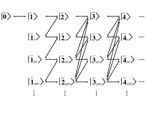
Figure 1: Schematic representation of the growth of the Hilbert space associated with the collective atomic states.

Eventually, all states of the Hilbert space will be visited by an arbitrary system evolution but, within a given time window, only a restricted portion of the Hilbert space will be accessed. However, in the example of Fig. 2, we observe that our approximation for the evolution of the collective atomic ground state is in good agreement with the exact result for very long times, reproducing even population collapses and revivals. Surprisingly, to achieve this level of accuracy, it is enough to consider the first two rows displayed in Fig. 1. The number of columns that has to be considered is determined by the number of initial excitations in the system because the Hamiltonian of Eq. (1) preserves this number. In consequence, the low mean photon number, $\bar{n}=1.8$, suggests that the initially unpopulated atomic state may reach at most a similar mean value. Given that the number of atoms is larger, $N=6$, it is expected that the normalized couplings between the few visited atomic states in the first row of Fig. 1 and the rows below are quite small. In order to confirm this intuition, we show in Fig. 3 how the population of the second and third rows of Fig. 1 decreases as the number of atoms $N$ increases for the same parameters of Fig. 2. Clearly, also increasing inhomogeneity of the coupling causes increased leakage into higher order rows, see Eq. (14). The example of Fig. 2 shows a reduction of the Hilbert space dimension from $2^{6}\times 7=448$, where $7$ is the dimension of the truncated field space, to an effective size of $49$. In general, to improve the accuracy, we only need to take into account more rows in the calculation.

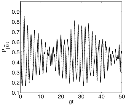
Figure 2: Evolution of the collective atomic ground state population, $P_{|\mathbf{\bar{0}}\rangle}$, in the case of inhomogeneous coupling $g_{j}=g\sin\left[j\pi/\left(N+1\right)\right]$, $j=1,..,N$, with $N=6$, an initial atomic state $\mathbf{\left|\mathbf{\bar{0}}\right\rangle}$, and an initial coherent state in the field with $\bar{n}=1.8$. Exact evolution (solid line) and approximated evolution (dotted line).

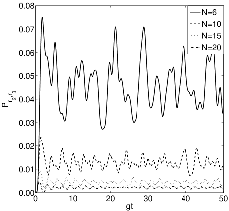
Figure 3: Evolution of the total population of the second and third rows, $P_{r_{2},r_{3}}$, for different number $N$ of atoms.

We have proposed a method to follow the dynamics of a system with inhomogeneous coupling in a relatively simple manner. It is now interesting to see how strong can be the effects of inhomogeneity on the dynamics of relevant observables. For example, in Fig. 4, we compare the different predictions for the fluctuations of the field quadratures. For the homogeneous case, the first time scale corresponds to $\sqrt{N}g$, while for the inhomogeneous case the analogous would be $(\sum_{j}g_{j}^{2})^{1/2}$. In this manner, to compare both cases, the homogeneous and the inhomogeneous we consider the homogeneous coupling case with coupling $g_{j}=1/(\sqrt{N})(\sum_{j}g_{j}^{2})^{1/2}$. In Fig. 4 we observe that not only does the inhomogeneous situation differ from the homogeneous in the typical timescale of the dynamics, but also it shows additional effects, which, in the case we consider, are reflected in an increase of the quadrature fluctuations. Our method allows the study of these effects for particle numbers that are non tractable for standard simulation methods.

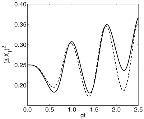
Figure 4: Evolution of the quadrature fluctuations $\left(\Delta X_{1}\right)^{2}=\left\langle X_{1}^{2}\right\rangle-\left\langle X_{1}\right\rangle^{2}$ for $N=8$, initial atomic ground state, and a coherent field with $\bar{n}=1$. Solid line: inhomogeneous coupling $g_{j}=g\sin\left[j\pi/\left(N+1\right)\right]$, where $j$ labels the position of the $j$-th atom. Dashed line: homogeneous case with $g_{j}=1/(\sqrt{N})(\sum_{j}g_{j}^{2})^{1/2}$.

III Quantum Dots

Another interesting physical system involving inhomogeneous coupling in a natural way is that of a single electron confined in a quantum dot surrounded by nuclear spins. In presence of a magnetic field $B_{0}$ along the $z$-axis the associated Hamiltonian, neglecting dipolar interactions between nuclear spins, can be written as CoishLoss ; Schliemann

$$\hat{H}_{\mathrm{QD}}=g^{\ast}\mu_{B}B_{0}\hat{S}_{z}+g_{n}\mu_{n}B_{0}\sum\limits_{i=1}^{N}\hat{I}_{z}^{(i)}+\hat{V}_{\mathrm{HF}}.$$ (18)

Here, the first two terms are the Zeeman energies of the electron and nuclear spins, and $\hat{V}_{\mathrm{HF}}=\hat{V}_{D}+\hat{V}_{\Omega}$ describes the hyperfine contact interaction of a single electron spin interacting with $N$ nuclear spins, where $\hat{V}_{D}=\sum_{i=1}^{N}\alpha_{i}\hat{I}_{z}^{(i)}\hat{S}_{z}$, and $\hat{V}_{\Omega}=\sum_{i=1}^{N}(\alpha_{i}/2)\left(\hat{I}_{-}^{(i)}\hat{S}_{+}+\hat{I}_{+}^{(i)}\hat{S}_{-}\right)$. The coefficients $\alpha_{i}=Av_{0}\left|\psi\left(\vec{r}_{i}\right)\right|^{2}$ are the inhomogeneous coupling constants, where $A$ is the hyperfine coupling constant, $v_{0}$ is the inverse density of nuclei in the material, and $\psi\left(\vec{r}_{i}\right)$ is the envelope function of the electron at position $\vec{r}_{i}$. The term $\hat{V}_{D}$ induces an effective magnetic field for the electron $\hat{B}_{\mathrm{eff}}=B_{0}+(1/g^{\ast}\mu_{B})\sum_{i=1}^{N}\alpha_{i}\hat{I}_{z}^{(i)}$, the so called Overhauser shift. Below, the nuclear Zeeman energies will be neglected, as their magnetic moment is much smaller than the one for the electron Schliemann .

By applying an appropriate field $B_{0}$, so that $g^{\ast}\mu_{B}\hat{B}_{\mathrm{eff}}\ll\hat{V}_{\Omega}$, one may allow the spin-exchange term to dominate the dynamics Taylor . In this case, and defining $\hat{A}_{\pm,z}=\sum_{j}\alpha_{j}\hat{I}_{\pm,z}^{(j)}$, the Hamiltonian of Eq. (18) approximately reduces to $\hat{V}_{\Omega}=(1/2)(\hat{A}_{-}\hat{S}_{+}+\hat{A}_{+}\hat{S}_{-})$. However, in general, the term $\hat{V}_{D}=\hat{A}_{z}\hat{S}_{z}$ cannot be neglected. Even on resonance, where $B_{0}=-(1/g^{\ast}\mu_{B})\langle\hat{A}_{z}\rangle$, one has $\langle\hat{A}_{z}^{2}\rangle-\langle\hat{A}_{z}\rangle^{2}\neq 0$. In conclusion, the Overhauser field felt by the electron spin cannot be fully compensated. To include this effect we rewrite the $zz$-part of the interaction as $\hat{A}_{z}=\bar{\alpha}\hat{J}_{z}+\delta\hat{A}_{z}=\bar{\alpha}\sum_{i=1}^{N}\hat{I}_{z}^{(i)}+\sum_{i}(\alpha_{i}-\bar{\alpha})\hat{I}_{z}^{(i)}$, so that the on-resonance Hamiltonian becomes

$$\widehat{\widetilde{H}}_{\mathrm{QD}}=\frac{1}{2}\left(\hat{A}_{-}\hat{S}_{+}+\hat{A}_{+}\hat{S}_{-}\right)+\bar{\alpha}\hat{S}_{z}(\hat{J}_{z}-\langle\hat{J}_{z}\rangle_{0})+\hat{V}_{zz}.$$ (19)

Here $\langle\hat{J}_{z}\rangle_{0}$ is the expectation value with respect to the fully polarized state, $\bar{\alpha}=\sum_{i}\alpha_{i}/N$ is the average coupling constant (which equals $A/N$ due to the normalization of the electron wave function), and $\hat{V}_{zz}=\hat{S}_{z}\delta\hat{A}_{z}$. The latter term, i.e. the inhomogeneous contribution to the $z$-term of the interaction, can be treated perturbatively. As we show later, the homogeneous $zz$-term $\hat{S}_{z}\hat{J}_{z}$ is neglected with respect to the flip-flop term due to a small factor $1/\sqrt{N}$. The term $\hat{V}_{zz}$ is even smaller and negligible, because it depends additionally on an inhomogeneity parameter, like the variance of the (smooth) electron wave function.

In this work we consider $I=1/2$ nuclear spins in a spherical quantum dot, and

$$\left|\psi(\vec{r})\right|^{2}\propto e^{-\frac{r^{2}}{r_{0}^{2}}},$$ (20)

as the electron envelope function Schliemann of size $r_{0}$.

III.1 Electron and Nuclear Spin Dynamics

The inhomogeneous coupling of the electron spin to the nuclear spins does not allow for a general analytical solution of the dynamics. The assumption of a fully polarized initial nuclear spin state reduces the dimension of the relevant Hilbert space from $2^{N+1}$ to $N+1$ and therefore the problem is readily analyzed. On the other hand, a more general initial state of nuclear spins vastly increases the dimension of the Hilbert space that the system will visit along the evolution. Motivated by the proposals for quantum information storage via the hyperfine interaction Taylor , we will study situations of imperfect, but high, polarization. We analyze the case where the dynamics involves one excitation in the nuclear spin system, which we will refer to as “defect”. We show, with methods similar to the ones developed in Sec. II, that the relevant Hilbert space remains still small.

The most general pure state describing this situation can be written as

$$\left|\mathbf{1}\right\rangle_{n}=\sum_{j=1}^{N}a_{j}\left|\mathbf{1}_{j}\right\rangle_{n},$$ (21)

with $\sum_{j=1}^{N}|a_{j}|^{2}=1$, and $\left|\mathbf{1}_{j}\right\rangle_{n}$ represents the state $\left|\downarrow\downarrow...\uparrow_{j}...\downarrow\downarrow\right\rangle_{n}$ with an inverted nuclear spin at position $r_{j}$. In particular we consider the case of a uniformly distributed defect $a_{j}=1/\sqrt{N}$ and a localized defect at position $j_{0}$,

$$a_{j}=C\left(\Gamma/2\right)^{2}/\left[\left(j-j_{0}\right)^{2}+\left(\Gamma/2\right)^{2}\right],$$ (22)

where $C$ is a normalization constant and $\Gamma$ characterizes the width of the distribution.

Let us consider two possible initial states for the electron and the nuclear spins with a single imperfection,

$$\left|\downarrow\right\rangle_{e}\left|\mathbf{1}\right\rangle_{n} \equiv \left|\downarrow\mathbf{1}\right\rangle,$$ (23)

$$\left|\uparrow\right\rangle_{e}\left|\mathbf{1}\right\rangle_{n} \equiv \left|\uparrow\mathbf{1}\right\rangle.$$ (24)

In order to solve the dynamical evolution of the composite system, we employ the recipe of following the relevant Hilbert space, as described in Sec. II. We observe that, under the action of the Hamiltonian of Eq. (19), the initial state $\left|\downarrow\mathbf{1}\right\rangle$ is coupled to the state $\left|\uparrow\mathbf{0}\right\rangle$ via $\hat{S}_{+}\hat{A}_{-}\left|\downarrow\mathbf{1}\right\rangle=\gamma\left|\uparrow\mathbf{0}\right\rangle$, with $\left|\mathbf{0}\right\rangle\equiv\left|\mathbf{0}\right\rangle_{n}=\left|\downarrow\downarrow...\downarrow\downarrow\right\rangle_{n}$ and

$$\gamma=\sum_{i}a_{i}\alpha_{i}.$$ (25)

The state $\left|\uparrow\mathbf{0}\right\rangle$ will be coupled through the term $\hat{S}_{-}\hat{A}_{+}$ to a state with one excitation, but different from $\left|\downarrow\mathbf{1}\right\rangle$. Similar to the formalism developed in Sec. II, we can write $\hat{S}_{-}\hat{A}_{+}\left|\uparrow\mathbf{0}\right\rangle=\gamma\left|\downarrow\mathbf{1}\right\rangle+\beta\left|\downarrow\mathbf{1}_{\bot}\right\rangle$, where state.

$$\left|\mathbf{1}_{\bot}\right\rangle=\frac{1}{\beta}\left(\sum_{i}\alpha_{i}\left|\mathbf{1}_{i}\right\rangle-\gamma\left|\mathbf{1}\right\rangle\right)$$ (26)

is orthogonal to state $\left|\mathbf{1}\right\rangle$, with $\beta=\sqrt{\left(N_{\mathbf{0}}\right)^{2}-\gamma^{2}}$ and $N_{\mathbf{0}}=\sqrt{\sum\limits_{i}\alpha_{i}^{2}}$. Finally, we observe that $\hat{S}_{+}\hat{A}_{-}\left|\downarrow\mathbf{1}_{\perp}\right\rangle=\beta\left|\uparrow\mathbf{0}\right\rangle$. In summary, the exchange terms yield

$$\hat{S}_{+}\hat{A}_{-}\left|\downarrow\mathbf{1}\right\rangle = \gamma\left|\uparrow\mathbf{0}\right\rangle,$$

$$\hat{S}_{-}\hat{A}_{+}\left|\uparrow\mathbf{0}\right\rangle = \gamma\left|\downarrow\mathbf{1}\right\rangle+\beta\left|\downarrow\mathbf{1}_{\bot}\right\rangle,$$

$$\hat{S}_{+}\hat{A}_{-}\left|\downarrow\mathbf{1}_{\bot}\right\rangle = \beta\left|\uparrow\mathbf{0}\right\rangle.$$ (27)

Furthermore, the $zz$-interaction yields matrix elements

$$\left\langle\downarrow\mathbf{1}\right|\bar{\alpha}\hat{S}_{z}(\hat{J}_{z}-\langle\hat{J}_{z}\rangle_{0})\left|\downarrow\mathbf{1}\right\rangle = -\frac{\bar{\alpha}}{2},$$

$$\left\langle\uparrow\mathbf{0}\right|\bar{\alpha}\hat{S}_{z}(\hat{J}_{z}-\langle\hat{J}_{z}\rangle_{0})\left|\uparrow\mathbf{0}\right\rangle = 0,$$

$$\left\langle\downarrow\mathbf{1}_{\bot}\right|\bar{\alpha}\hat{S}_{z}(\hat{J}_{z}-\langle\hat{J}_{z}\rangle_{0})\left|\downarrow\mathbf{1}_{\bot}\right\rangle = -\frac{\bar{\alpha}}{2}.$$ (28)

Therefore, for the initial condition of Eq. (23) the system evolves only in the subspace spanned by $\left\{\left|\downarrow\mathbf{1}\right\rangle,\left|\uparrow\mathbf{0}\right\rangle,\left|\downarrow\mathbf{1}_{\bot}\right\rangle\right\}$. The temporal evolution in this subspace can be exactly solved, obtaining $\left|\Psi_{\downarrow}\left(t\right)\right\rangle_{e-n}=a_{1}(t)\left|\downarrow\mathbf{1}\right\rangle+b_{1}(t)\left|\uparrow\mathbf{0}\right\rangle+c_{1}(t)\left|\downarrow\mathbf{1}_{\bot}\right\rangle$, where the probability amplitudes are given by

$$a_{1}(t) = \!\!1+\frac{\gamma^{2}\exp\left(i\bar{\alpha}t/4\right)}{\Omega^{2}\delta}[\delta\cos\left(\delta t/2\right)$$

$$+i\frac{\bar{\alpha}}{2}\sin\left(\delta t/2\right)-\delta\exp\left(-i\bar{\alpha}t/4\right)],$$

$$b_{1}(t) = \!\!-i\frac{\gamma}{\delta}\exp\left(i\bar{\alpha}t/4\right)\sin\left(\delta t/2\right),$$

$$c_{1}(t) = \!\!\frac{\gamma\beta\exp\left(i\bar{\alpha}t/4\right)}{\Omega^{2}\delta}[\delta\cos\left(\delta t/2\right)+i\frac{\bar{\alpha}}{2}\sin\left(\delta t/2\right)$$ (29)

$$-\delta\exp\left(-i\bar{\alpha}t/4\right)].$$

Here, $\Omega=\sqrt{\gamma^{2}+\beta^{2}}=N_{0}$ and $\delta=\sqrt{\left(\bar{\alpha}/2\right)^{2}+\Omega^{2}}$ plays the role of a generalized Rabi frequency for a process with detuning $\bar{\alpha}$. The $zz$-interaction thus leads to a small detuning for the exchange of excitation between electron and nuclear spins: We have that $\Omega=\sqrt{\gamma^{2}+\beta^{2}}=N_{0}=\sqrt{\sum_{i}\alpha_{i}^{2}}$. The $\alpha_{i}$ are $\mathcal{O}(1/N)$, such that $\sum_{i}\alpha_{i}^{2}=\mathcal{O}(1/N)$. When $N\gg 1$, then $1/N=\bar{\alpha}\ll\Omega=\mathcal{O}(1/\sqrt{N})$. It is important to notice that in the case of an initially fully polarized nuclear state $\left|\mathbf{0}\right\rangle$ and the electron spin in $\left|\downarrow\right\rangle_{e}$ the system is not affected by the exchange interaction terms $\hat{S}_{-}\hat{A}_{+}$ and $\hat{S}_{+}\hat{A}_{-}$.

On the other hand, if the system is initially in the state $\left|\uparrow\right\rangle_{e}\left|\mathbf{1}\right\rangle_{n}$, the coupling through the Hamiltonian of Eq. (19) does not lead to a closed Hilbert space. Then, some approximations are necessary in order to obtain solutions for the evolution of the overall system dynamics. Starting from $\left|\uparrow\mathbf{1}\right\rangle$, we have

$$\hat{S}_{-}\hat{A}_{+}\left|\uparrow\mathbf{1}\right\rangle=\left|\downarrow\right\rangle\sum_{i<j}b_{ij}\left|\mathbf{2}_{ij}\right\rangle,$$ (30)

where $b_{ij}=a_{i}\alpha_{j}+a_{j}\alpha_{i}$ and $\left|\mathbf{2}_{ij}\right\rangle=\left|\downarrow\downarrow...\uparrow_{i}...\uparrow_{j}...\downarrow\downarrow\right\rangle$. Defining

$$\left|\mathbf{2}\right\rangle=\sum_{i<j}c_{ij}\left|\mathbf{2}_{ij}\right\rangle,$$ (31)

with $c_{ij}=b_{ij}/N_{\mathbf{2}}$ and $N_{\mathbf{2}}=\sqrt{\sum\limits_{i<j}b_{ij}^{2}}$, we observe that the state $\left|\downarrow\mathbf{2}\right\rangle$ is coupled only through

$$\hat{S}_{+}\hat{A}_{-}\left|\downarrow\mathbf{2}\right\rangle=\sum_{i}(\sum_{j\neq i}c_{ij}\alpha_{j})\left|\uparrow\mathbf{1}_{i}\right\rangle\equiv\left|\uparrow\phi_{1}\right\rangle.$$ (32)

Here, $\left|\phi_{1}\right\rangle$ can be seen as having one component along the state $\left|\mathbf{1}\right\rangle$ and other component along orthogonal state $\left|\mathbf{1}_{p}\right\rangle$ , such that

$$\left|\phi_{1}\right\rangle=\left\langle\mathbf{1}\right.\left|\phi_{1}\right\rangle\left|\mathbf{1}\right\rangle+\sqrt{\left\langle\phi_{1}\right.\left|\phi_{1}\right\rangle-\left\langle\mathbf{1}\right.\left|\phi_{1}\right\rangle^{2}}\left|\mathbf{1}_{p}\right\rangle,$$ (33)

where $\left|\mathbf{1}_{p}\right\rangle=\left(1/N_{\mathbf{1}_{p}}\right)\left(\left|\phi_{1}\right\rangle-\left\langle\mathbf{1}\right.\left|\phi_{1}\right\rangle\left|\mathbf{1}\right\rangle\right)$, with $N_{\mathbf{1}_{P}}=\sqrt{\left\langle\phi_{1}\right.\left|\phi_{1}\right\rangle-\left\langle\mathbf{1}\right.\left|\phi_{1}\right\rangle^{2}}$. Following this procedure, we have

$$\hat{S}_{-}\hat{A}_{+}\left|\uparrow\mathbf{1}_{p}\right\rangle=\left|\downarrow\mathbf{2}\right\rangle+N_{\mathbf{2}_{p}}\left|\downarrow\mathbf{2}_{p}\right\rangle\equiv\left|\uparrow\phi_{2}\right\rangle,$$ (34)

where $\left|\mathbf{2}_{p}\right\rangle=\left(1/N_{\mathbf{2}_{P}}\right)\left(\left|\phi_{2}\right\rangle-\left\langle\mathbf{2}\right.\left|\phi_{2}\right\rangle\left|\mathbf{2}\right\rangle\right)$, with $\left|\phi_{2}\right\rangle=\hat{A}_{+}\left|\mathbf{1}_{p}\right\rangle$ and $N_{\mathbf{2}_{P}}=\sqrt{\left\langle\phi_{2}\right.\left|\phi_{2}\right\rangle-\left\langle\mathbf{2}\right.\left|\phi_{2}\right\rangle^{2}}$. In order to implement a semi-analytical description for the overall system dynamics we have to truncate the Hilbert space. This can be accomplished by approximating the action of $\hat{S}_{+}\hat{A}_{-}$ over $\left|\mathbf{2}_{p}\right\rangle$ such that

$$\hat{S}_{+}\hat{A}_{-}\left|\downarrow\mathbf{2}_{p}\right\rangle = N_{\mathbf{2}_{P}}\left|\uparrow\mathbf{1}_{p}\right\rangle+N_{\mathbf{1}pp}\left|\uparrow\mathbf{1}_{pp}\right\rangle$$ (35)

$$\simeq N_{\mathbf{2}_{P}}\left|\uparrow\mathbf{1}_{p}\right\rangle,$$

where the state $\left|\uparrow\mathbf{1}_{pp}\right\rangle$ is similarly defined in terms of $\left|\uparrow\mathbf{1}_{p}\right\rangle$. This approximation can be justified from Fig. 5 where we have plotted the total occupation probability of states within the subspace of first orthogonal states $\left|\uparrow\mathbf{1}\right\rangle,\left|\downarrow\mathbf{2}\right\rangle,\left|\uparrow\mathbf{1}_{p}\right\rangle,\left|\downarrow\mathbf{2}_{p}\right\rangle$. As all of them are eigenstates of the $\hat{J}_{z}$ term, its effect is again a small detuning. These results have been obtained by numerical calculation considering a 12-dimensional truncated Hilbert space up to $\left|\downarrow\mathbf{2}_{ppppp}\right\rangle$. However, if we use a Hilbert space truncated up to $\left|\downarrow\mathbf{2}_{pp}\right\rangle$, the total occupation probability of the mentioned subspace is practically the same as shown in Fig. 5.

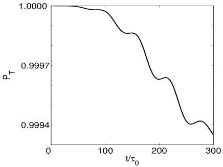
Figure 5: Total population $P_{\rm T}$ of the states $\left\{\left|\uparrow\mathbf{1}\right\rangle,\left|\downarrow\mathbf{2}\right\rangle,\left|\uparrow\mathbf{1}_{p}\right\rangle,\left|\downarrow\mathbf{2}_{p}\right\rangle\right\}$, with $N=10^{3}$ and defect distribution $a_{j}=1/\sqrt{N}$.

We have seen before that the typical timescale for the exchange of an excitation between the electron and nuclei is given by the inverse of the generalized Rabi frequency

$$\tau:=\pi/\Omega=\pi/N_{0}.$$ (36)

From Fig. 5 we deduce that the dynamics of the composite system is well described for times beyond $\tau$, which is important for our subsequent analysis of the quantum memory. In particular, for the case $N=10^{3}$, this time is approximately $\tau\approx 68\tau_{0}$, with $\tau_{0}=\hbar/A$, and we are allowed to restrict the dynamics to the subspace spanned by $\left\{\left|\uparrow\mathbf{1}\right\rangle,\left|\downarrow\mathbf{2}\right\rangle,\left|\uparrow\mathbf{1}_{p}\right\rangle,\left|\downarrow\mathbf{2}_{p}\right\rangle\right\}$. This is an important feature of our method, since numerical calculations are significantly simplified.

III.2 Quantum Information Storage

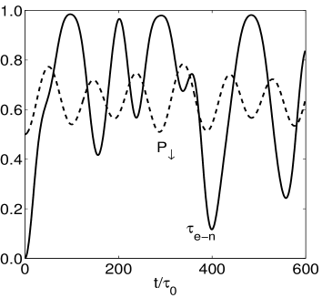
Figure 6: Evolution of the tangle $\tau_{e-n}$ (solid line) and  population $P_{\downarrow}$ of $\left|\downarrow\right\rangle_{e}$ (dashed line) for a uniformly distributed defect. The initial state is $\left|\Psi\right\rangle=1/\sqrt{2}\left(\left|\uparrow\right\rangle+\left|\downarrow\right\rangle\right)_{e}\otimes\left|\mathbf{1}\right\rangle_{n}$, $N=10^{3}$, and $\tau\sim 68\tau_{0}$.

In Refs. Taylor a long-lived quantum memory based on the capability that an electronic spin state can be reversibly mapped into a fully-polarized nuclei state was proposed. This dynamics can be expressed as

$$\left(u\left|\uparrow\right\rangle+v\left|\downarrow\right\rangle\right)\otimes\left|\mathbf{0}\right\rangle\rightarrow\left|\downarrow\right\rangle\left(v\left|\mathbf{1}\right\rangle+iu\left|\mathbf{0}\right\rangle\right)$$ (37)

where $\left|\mathbf{1}\right\rangle=\left(1/N_{\mathbf{0}}\right)\sum_{i}\alpha_{i}\left|\mathbf{1}_{i}\right\rangle$. This coherent mapping is effected by pulsing the applied field from $g^{\ast}\mu_{B}B_{\mathrm{eff}}\gg\hat{V}_{\Omega}$ to $B_{\mathrm{eff}}\sim 0$ for a time $\tau=\pi/N_{\mathbf{0}}$. Here, we study this dynamics in the context of an initial distributed single defect in the nuclear spin state. For the transfer process to be successful it is necessary that the electronic state factorizes from the nuclear spin state, thus requiring that at some point of the evolution

$$\left(u\left|\uparrow\right\rangle+v\left|\downarrow\right\rangle\right)\otimes\left|\mathbf{1}\right\rangle_{n}\rightarrow\left\{\begin{array}[]{c}\left|\downarrow\right\rangle_{e}\otimes\left|\psi^{\downarrow}_{u,v}\right\rangle_{n}\\ \left|\uparrow\right\rangle_{e}\otimes\left|\psi^{\uparrow}_{u,v}\right\rangle_{n}\,.\end{array}\right.$$ (40)

In order to verify if this is possible we analyze the populations of the electron spin and study the entanglement between the electron and the nuclear spins. Since the overall system is in a pure state we can use as an entanglement measure the tangle Rungta , $\tau_{AB}$=$2\nu_{A}\nu_{B}\left[1-\text{{tr}}\left(\rho_{A}^{2}\right)\right]$, where $\rho_{A}$ is the reduced density operator after tracing over subsystem $B$, and $\nu_{A}$ and $\nu_{B}$ are arbitrary scale factors set to $\nu_{A}=\nu_{B}=1$.

We first consider the case of a uniformly distributed initial nuclear spin excitation. In Fig. 6 we show the electron spin population $p_{\downarrow}$ and the tangle between the electron and $N=10^{3}$ nuclear spins. We observe that, for the case of a uniformly distributed defect, there is no time for which the composite state evolves to a factorized state as in Eq. (40). The electron spin population is never maximal or minimal (in both cases the tangle would vanish), meaning that there is no high-fidelity information transfer to the nuclei.

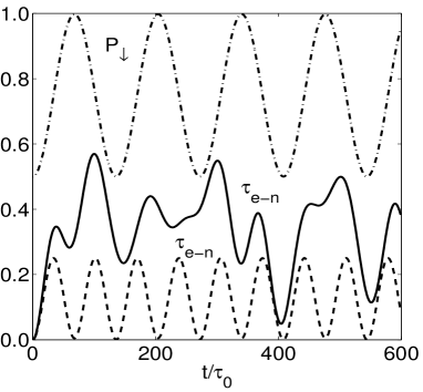
Figure 7: Evolution of the tangle $\tau_{e-n}$ for a defect distribution peaked at the edge of the quantum dot. Shown are the electron spin population $P_{\downarrow}$ (dot-dashed line) and the tangle (dashed line) for a defect distribution width $\Gamma=N/50$, and the tangle for the width $\Gamma=N$ (solid line) for $N=10^{3}$ and the initial state $\left|\Psi\right\rangle=1/\sqrt{2}\left(\left|\uparrow\right\rangle+\left|\downarrow\right\rangle\right)_{e}\otimes\left|\mathbf{1}\right\rangle_{n}$.

We study now the transfer process for the case of a localized defect as shown in Eq. (22). When the defect is peaked in the center of the dot, information storage is seriously hindered. However, if the defect is more probably located at an extreme of the quantum dot, the coupling of the defect-spin to the electron is weak, and separability is reached even for rather broad defect distributions, as seen in Fig. 7. The necessary conditions for a successful transfer are fulfilled after a time $t\approx 68\tau_{0}$, which is very close to the transfer time for an initial fully polarized nuclear spin state given by Eq. (36).

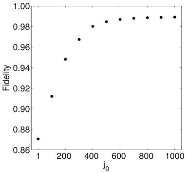
Figure 8: Fidelity of the quantum memory for $N=10^{3}$ nuclear spins and different $j_{0}$, $1\leq j_{0}\leq N$.

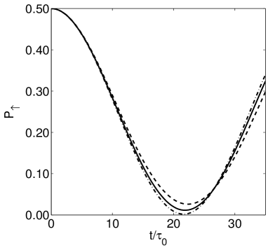
Figure 9: Evolution of the population $P_{\uparrow}$ of the electronic spin state $\left|\uparrow\right\rangle_{e}$ for $N=40$. The initial state for the electron spin is $\left|\Psi\right\rangle_{e}=1/\sqrt{2}\left(\left|\uparrow\right\rangle+\left|\downarrow\right\rangle\right)_{e}$ and $\rho_{N}=\sum_{j=1}^{N}a_{j}\hat{\sigma}_{+}^{\left(j\right)}\left|\mathbf{0}\right\rangle\left\langle\mathbf{0}\right|\hat{\sigma}_{-}^{\left(j\right)}$ for the nuclear spins. Solid line: $a_{j}=1/N$; Dashed line: $a_{j}=[C\left(\Gamma/2\right)^{2}/(\left(j-j_{0}\right)^{2}+\left(\Gamma/2\right)^{2})]^{2}$, with $\Gamma=N$   $j_{0}=1$, and $C$ a normalization constant. Dot-dashed line: same as for dashed line but $j_{0}=N$.

The performance of the quantum information storage protocol is analyzed now in a more quantitative manner by simulating a complete cycle of write-in, storage and retrieval. In the first step the electron spin in state $|\psi_{i}\rangle$ interacts with the nuclei and after a time $\tau$ the evolution is interrupted and the electron traced out. Then a fresh electron in state $|\downarrow\rangle$ interacts with the nuclei and after another time $\tau$ the nuclei are traced out. The fidelity $F=\langle\psi_{i}|\rho_{f}|\psi_{i}\rangle$ between this final electron spin state $\rho_{f}$ and the initial state is plotted in Fig. 8 for various defect distributions, where $F$ has been calculated by averaging on the electron spin Bloch sphere.

In Fig. 9 we consider the nuclear spins in a mixed state where electron spin populations are displayed. This figure shows that the electron spin performs very regular Rabi oscillations that deviate only slightly from the ideal situation with no defect present. In particular the performance is better than in the corresponding cases of coherently distributed defects. This is to be expected as the quantum information storage is sensitive to the coherences of the nuclear spins state, and they are absent in this mixed state case. Note that in Fig. 9 the initial number of nuclear spin excitations is fixed, at variance with a thermal distribution. In this case the visited Hilbert space scales as $N^{2}$ and not as $2^{N+1}$, allowing an exact calculation.

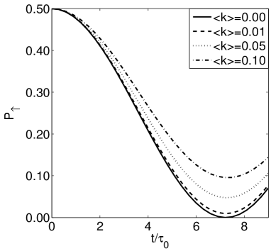
Figure 10: Evolution of population $P_{\uparrow}$ of electronic spin state $\left|\uparrow\right\rangle_{e}$ for an initial thermal distribution for each nuclear spin $N=10$ and different $\left\langle k\right\rangle$. The initial electron spin state is $\left|\Psi\right\rangle=1/\sqrt{2}\left(\left|\uparrow\right\rangle+\left|\downarrow\right\rangle\right)_{e}$. For this case, $\left\langle k\right\rangle=\exp\left(-\beta\hbar\omega\right)/\left(1+\exp\left(-\beta\hbar\omega\right)\right).$

Another possible physical scenario is that of an initial nuclear system at finite temperature. Our method is not directly applicable to that situation because already the initial state covers a large part of the Hilbert space. Nevertheless, for the sake of completeness, we include a brief analysis of this case in the context of a quantum memory in the presence of defects. Consider a thermal state for each nuclear spin

$$\rho_{\text{{th}}}^{i}=\frac{e^{-\hbar\omega\hat{\sigma}_{z}^{i}\beta}}{\text{{tr}}(e^{-\hbar\omega\hat{\sigma}_{z}^{i}\beta})}$$ (41)

with $\beta=1/k_{B}T$, where $T$ is the associated temperature. The average population of each spin is $\langle k\rangle=\langle\hat{\sigma}_{z}^{(i)}\rangle+1/2$. As for the initial mixed state case of Fig. 8, it is not possible to define collective states as was the case for pure initial states. The results of our direct simulations taking into account the whole Hilbert space are shown in Fig. 10, where we show the population of the electronic spin state $\left|\uparrow\right\rangle$. For nuclear polarizations above 95% the contrast of the Rabi oscillations of the electron spin deviate from the ideal situation by only a few percent. The scaling of the error with the particle number $N$ is certainly beyond the scope of this article.

IV CONCLUSIONS

We have developed a technique, based on suitable inspection and truncation of the associated Hilbert space, that allows to follow the quantum evolution of interacting systems with inhomogeneous coupling in an accurate and controlled manner. As a first general case, we illustrated the proposed method for the inhomogeneous Tavis-Cummings model and showed how the statistical properties may change appreciably depending on the spatial coupling distribution. As a second major example, we studied the dynamics of an electron spin interacting inhomogeneously with a system of polarized nuclear spins in a quantum dot, previously considered as a quantum memory candidate. We found that the reliability of the storage process depends strongly on the presence and position of a single distributed defect in the polarized nuclei state. The proposed technique may be easily extended to other inhomogeneously interacting systems and may prove to be accurate and efficient when interaction times are known beforehand, as is the case of pulses.

- (1) J. M. Raimond, M. Brune, and S. Haroche, Rev. Mod. Phys. 73, 565 (2001).
- (2) D. Leibfried, R. Blatt, C. Monroe, and D. Wineland, Rev. Mod. Phys. 75, 281 (2003).
- (3) V. Cerletti, W. A Coish, O. Gywatt, and D. Loss, Nanotechnology 16, R27 (2005).
- (4) A. Blais, R.-S. Huang, A. Wallraff, S.M. Girvin, and R.J. Schoelkopf, Phys. Rev. A 69, 062320 (2004).
- (5) E.T. Jaynes and F.W. Cummings, Proc. IEEE 51, 89 (1963).
- (6) B. W. Shore and P. L. Knight, J. Mod. Opt. 40, 1195 (1993).
- (7) R. H. Dicke, Phys. Rev. 93, 99 (1954).
- (8) M. Tavis and F.W. Cummings, Phys. Rev. 170, 379 (1968).
- (9) M. Orszag, R. Ramírez, J.C. Retamal, and C. Saavedra, Phys Rev. A 49, 2933 (1994).
- (10) J.C. Retamal, C. Saavedra, A.B. Klimov and S.M. Chumakov, Phys. Rev. A 55, 2413 (1997).
- (11) C. Saavedra, A.B. Klimov, S.M. Chumakov and J.C. Retamal, Phys. Rev. A 58, 4078 (1998).
- (12) A. Retzker, E. Solano, and B. Reznik, Phys. Rev. A, 75, 022312 (2007).
- (13) S.A. Wolf, D.D. Awschalom, R.A. Buhrman, J.M. Daughton, S. von Molnár, M.L. Roukes, A.Y. Chtchelkanova, and D.M. Treger, Science 294, 1488 (2001).
- (14) D. Loss and D.P. DiVincenzo, Phys. Rev. A 57, 120 (1998).
- (15) B. Kane, Nature (London) 393, 133 (1998).
- (16) J. M. Taylor, G. Giedke, H. Christ, B. Paredes, J. I. Cirac, P. Zoller, M. D. Lukin, and A. Imamoglu, cond-mat/0407640 (2004).
- (17) V. Privman, I. D. Vagner, and G. Kventsel, Phys. Lett. A 239, 141 (1998).
- (18) J. Levy, Phys. Rev. A 64, 052306 (2001).
- (19) T.D. Ladd, J.R. Goldman, F. Yamaguchi, Y. Yamamoto, E. Abe, and K.M. Itoh, Phys. Rev. Lett. 89, 017901 (2002).
- (20) J.M. Taylor, C.M. Marcus, and M.D. Lukin, Phys. Rev. Lett. 90, 206803 (2003); J.M. Taylor, A. Imamoglu, and M.D. Lukin, Phys. Rev. Lett. 91, 246802 (2003).
- (21) R. Mani, W. Johnson, V. Narayanamurti, Superlatt. & Microstructures, 32, 261 (2002); R. Mani, W. Johnson, V. Narayanamurti, V. Privman, and Y-M. Zhang, Physica E, 12, 152 (2002).
- (22) A. Imamoglu, E. Knill, L. Tian, and P. Zoller, Phys. Rev. Lett. 91, 017402 (2003).
- (23) H. Christ, J. I. Cirac, and G. Giedke, cond-mat/0611438 (2006).
- (24) C. Deng, and X. Hu, Phys. Rev. B 71, 033307 (2005), cond-mat/0402428.
- (25) C. W. Lai, P. Maletinsky, A. Badolato, A. Imamoglu, Phys. Rev. Lett. 96, 167403 (2006); A. S. Bracker, E. A. Stinaff, D. Gammon, M. E. Ware, J. G. Tischler, A. Shabaev, Al. L. Efros, D. Park, D. Gershoni, V. L. Korenev, and I. A. Merkulov, Phys. Rev. Lett 94, 047402 (2005); P.-F. Braun, B. Urbaszek, T. Amand, X. Marie, O. Krebs, B. Eble, A. Lemaitre, P. Voisin, cond-mat/0607728 (2006).
- (26) J. Schliemann, A.V. Khaetskii, and D. Loss, J. Phys.: Condens. Matter 15, R1809 (2003); J. Schliemann, A.V. Khaetskii, and D. Loss, Phys. Rev. B 66, 245303 (2002).
- (27) W.A. Coish and D. Loss, Phys. Rev. B 70, 195340 (2004).
- (28) P. Rungta, V. Buzek, C.M. Caves, M. Hillery, and G.J. Milburn, Phys. Rev. A 64, 042315 (2003).