Quantification of Continuous Variable Entanglement with only Two Types of Simple Measurements

Abstract

Here we propose an experimental set-up in which it is possible to obtain the entanglement of a two-mode Gaussian state, be it pure or mixed, using only simple linear optical measurement devices. After a proper unitary manipulation of the two-mode Gaussian state only number and purity measurements of just one of the modes suffice to give us a complete and exact knowledge of the state’s entanglement.

,

1 Introduction

Quantum theory of information offers, in principle, a plethora of resources for the processing of computational and informational tasks in an efficient way, otherwise unattainable in the classical world [1, 2, 3, 4]. Initially, all the quantum communication protocols were developed for discrete systems (qubits) and later an equivalent formulation for the quantum continuous variable (CV) setting was developed. CV-systems are described by canonical conjugate operators like position and momentum or the quadrature amplitudes of the quantized electromagnetic field. The main reason for the development of a CV quantum information theory are of a practical order: the crucial steps in quantum communication protocols are relatively simple to implement via the available experimental techniques of quantum optics [2]. Some of these tasks, e.g. quantum cryptography [5, 6, 7], superdense coding [8, 9, 10] and teleportation [11, 12, 13], require entanglement as a key ingredient for their successful implementation. Therefore, a great deal of effort has been put into the qualitative and quantitative study of entanglement. However, it is still a difficult problem to obtain in a simple experimental fashion the degree of entanglement of a quantum system. Practically all the useful entanglement measures developed so far can only be computed with a complete knowledge of the quantum state, whose reconstruction is not a trivial experimental task.

A direct scheme for the measurement of the entanglement of a pair of pure qubits, without state reconstruction, was recently proposed [14] and experimentally realized [15]. For continuous variable systems (CV-systems), being Gaussian states a famous example which are efficiently generated in the laboratory [2, 4], interesting experimental proposals for the measurement of entanglement were presented [16, 17, 18] and implemented [19] recently. In particular, it was shown that by measuring the marginal (local) and global purities of a two-mode Gaussian state one is able to estimate the state negativity [20], although its exact value cannot be achieved via this procedure. The negativity, together with the entanglement of formation [21], are the most important entanglement measures for Gaussian states, where the latter is only analytically computable for symmetric Gaussian states.

Here we present a simple experimental scheme allowing the measurement of the exact value of the entanglement of formation for an arbitrary symmetric two-mode Gaussian state. In fact, the scheme can also be adapted to obtain the exact value of the negativity for an arbitrary two-mode Gaussian state as well, being it symmetric or not. The only prior knowledge needed for entanglement quantification, which is also a requisite of all previous schemes, is upon the Gaussian nature of the two-mode state. Whether it is a pure or a mixed state is irrelevant for our purposes. Furthermore, even if we do not know that we are dealing with a Gaussian state our method can be used to experimentally apply the Simon separability test [22], which is a sufficient condition for the existence of CV-entanglement.

A most remarkable feature of our scheme, which differentiates it from previous proposals, is that all the information relevant to the exact quantification of the entanglement of the state can be obtained, after a non-local unitary operation on the two-modes, via local projective measurements. After combining the two-modes in a beam splitter (non-local unitary operation) the entanglement can be quantified solely by measurements of the purity and the number of photons of just one of the modes. Therefore, all the information concerning the entanglement of the two-modes is transferred to local properties of one of the modes after a non-local unitary operation. It is in this sense that the entanglement can be seen as determined by two single types of local projective measurements with no need for quantum state reconstruction or, equivalently, without the knowledge of the two-mode covariance matrix.

2 Entanglement of a two-mode Gaussian state

A two-mode Gaussian state $\rho$ is completely characterized by its covariance matrix, with elements $\gamma_{ij}$ $=$ $\langle R_{i}R_{j}+R_{j}R_{i}\rangle_{\rho}$ $-$ $2$$\langle R_{i}\rangle_{\rho}$$\langle R_{j}\rangle_{\rho}$, where $\langle R_{i}\rangle_{\rho}$ is the quantum expectation value of the observable $R_{i}$ and $(R_{1},R_{2},R_{3},R_{4})$ $=$ $(X_{1},P_{1},X_{2},P_{2})$ are the quadratures of the electromagnetic field modes [23]. Any covariance matrix can be brought via local symplectic transformations, i.e. without affecting its entanglement content, to the standard form [22]

$$\gamma=\left(\begin{array}[]{cc}A&C_{\gamma}\\ C_{\gamma}^{T}&B\end{array}\right),$$ (1)

where $A,B$, and $C_{\gamma}$ are $2\times 2$ real diagonal matrices given as [21] $A=\mbox{diag}(n,n)$, $B=\mbox{diag}(m,m)$, and $C_{\gamma}=\mbox{diag}(k_{x},-k_{p})$. It can be shown [22] that a two-mode Gaussian state is not entangled if $k_{x}k_{p}\geq 0$. However, it may or may not be entangled when $k_{x}k_{p}<0$. A Gaussian state is not entangled (separable) if, and only if [22]

$$I_{1}I_{2}+(1-|I_{3}|)^{2}-I_{4}\geq I_{1}+I_{2},$$ (2)

where $I_{1}=\mbox{det}(A)$, $I_{2}=\mbox{det}(B)$, $I_{3}=\mbox{det}(C_{\gamma})$ and $I_{4}=\mbox{tr}(AJC_{\gamma}JBJC_{\gamma}^{T}J)$ are the four invariants of the $Sp(2,R)\otimes Sp(2,R)$ group [22]. Here $J$ is an anti-diagonal $2\times 2$ matrix given by $J=\mbox{adiag}(1,-1)$, $\mbox{det}(M)$ stands for the determinant of the matrix $M$, $\mbox{tr}(M)$ is the trace of $M$, and $M^{T}$ is the transpose of $M$.

For a symmetric state ($I_{1}=I_{2}$) the entanglement of formation [21] can be written in terms of the symplectic invariants as [24]

$$E_{f}(\rho)=f\left(\sqrt{I_{1}+|I_{3}|-\sqrt{I_{4}+2\,I_{1}\,|I_{3}|}}\right),$$ (3)

where $f(x)=c_{+}(x)\log_{2}(c_{+}(x))-c_{-}(x)\log_{2}(c_{-}(x))$ and $c_{\pm}(x)=(x^{-1/2}\pm x^{1/2})^{2}/4$. There is no analytical expression of $E_{f}$ for non-symmetric Gaussian states. However, their entanglement can be quantified by the negativity, which can be calculated if the above four symplectic invariants are known [16, 17].

3 The four local invariants

It is important to note, since this is a crucial ingredient of our experimental proposal, that the four quantities $I_{1}$, $I_{2}$, $I_{3}$, and $I_{4}$ are invariants by local symplectic transformations in the quadratures, or equivalently, they are invariant by local unitary operations in the density matrix $\rho$ [22]. The knowledge of these four invariants allows us to completely characterize the entanglement properties of a two-mode Gaussian state: we can discover if it is entangled (Eq. (2)) as well as how much it is entangled (Eq. (3)). Therefore, the measurement of these symplectic invariants is the base on which our proposal is built and our goal now is to present an experimental set-up in which they can be easily determined.

For this purpose it is more appropriate to work with the covariance matrix $V$ [25] of the creation, $a_{j}^{\dagger}=(X_{j}-\mathrm{i}P_{j})/\sqrt{2}$, and annihilation, $a_{j}=(X_{j}+\mathrm{i}P_{j})/\sqrt{2}$, operators for the two modes ($j=1,2$) [26]. Defining $\mathbf{v}=$ $(v_{1},v_{2},v_{3},v_{4})^{T}$ $=$ $(a_{1},a_{1}^{\dagger},a_{2},a_{2}^{\dagger})^{T}$, the matrix elements of $V$ are $V_{ij}=(-1)^{i+j}\langle v_{i}v_{j}^{\dagger}+v_{j}^{\dagger}v_{i}\rangle_{\rho}/2$ [27]. As we did for $\gamma$ we can represent $V$ in terms of four block matrices of dimension two:

$$V=\left(\begin{array}[]{cc}V_{1}&C_{V}\\ C_{V}^{\dagger}&V_{2}\end{array}\right).$$ (4)

In this new representation the four symplectic invariants read: $J_{1}=\mbox{det}(V_{1})$, $J_{2}=\mbox{det}(V_{2})$, $J_{3}=\mbox{det}(C_{V})$ and $J_{4}=\mbox{tr}(V_{1}ZC_{V}ZV_{2}ZC_{V}^{\dagger}Z)$, where $Z=\mbox{diag}(1,-1)$. Recalling the definitions of $\gamma_{ij}$, $V_{ij}$, and the relation between $X_{j},P_{j}$ and $a_{j},a_{j}^{\dagger}$ it is straightforward to see that

$$I_{1}=4J_{1},\,I_{2}=4J_{2},\,I_{3}=4J_{3},\,I_{4}=16J_{4}.$$ (5)

Like $\gamma$, under local symplectic transformations $V$ can be brought to the following standard form [28]:

$$\tilde{V}=\left(\begin{array}[]{cc}\tilde{V}_{1}&\tilde{C}_{V}\\ \tilde{C}_{V}^{\dagger}&\tilde{V}_{2}\end{array}\right),$$ (6)

with

$$\tilde{V}_{1}=\left(\begin{array}[]{cc}\tilde{n}_{1}&0\\ 0&\tilde{n}_{1}\end{array}\right),\tilde{V}_{2}=\left(\begin{array}[]{cc}\tilde{n}_{2}&0\\ 0&\tilde{n}_{2}\end{array}\right),\tilde{C}_{V}=\left(\begin{array}[]{cc}\tilde{m}_{s}&\tilde{m}_{c}\\ \tilde{m}_{c}&\tilde{m}_{s}\end{array}\right),$$

where $\tilde{m}_{s}$ and $\tilde{m}_{c}$ are real parameters. From now on, whenever we deal with the standard form of $V$, we will write its elements as well as any related quantity thereof with a tilde ($\tilde{\,}$).

4 Experimental proposals

We only need, then, to experimentally measure $J_{1}$, $J_{2}$, $J_{3}$, and $J_{4}$ to completely quantify the entanglement of a two-mode Gaussian state. We first show a scheme in which we can determine the first three invariants. With these three invariants, as will be shown in what follows, we can obtain bounds for the entanglement of a two-mode Gaussian state. We then introduce two local unitary operations to the previous scheme, allowing us to determine $J_{4}$, the remaining invariant.

4.1 First scheme

The experimental set-up necessary to measure the first three invariants is very simple and is depicted in Fig. 1. It can be thought of as a simplification of the scheme presented in Ref. [29] to reconstruct the two-mode covariance matrix of a Gaussian state. Here, however, there is no state reconstruction and we only use linear optical devices to measure the purity and the photon number of the output mode $a^{\prime}_{1}$. Loosely speaking the linear optics apparatus (adjustable phase shifter and a beam splitter) can be seen as the agent responsible for transferring the entanglement properties between the two modes $a_{1}$ and $a_{2}$ to the mode $a^{\prime}_{1}$ [26]. On the other hand, the measuring apparatus (photon counting and/or homodyne detection) are responsible for the local projective measurements which determine these properties.

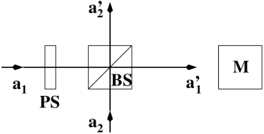
Figure 1: Experimental set-up to measure three symplectic invariants ($J_{1}$, $J_{2}$, and $J_{3}$) of a two-mode Gaussian state. Input modes $a_{1}$ and $a_{2}$ pass through a beam splitter (BS) with transmittance $\cos\theta$. Before reaching the BS mode $a_{1}$ passes through a phase-shifter (PS) acquiring a phase $\varphi$. After the BS measurements (M) are made on the output mode $a^{\prime}_{1}$ only. Two types of measurements are required to completely characterize the invariants of the input two-mode Gaussian state: the photon number and the purity (Wigner function at the origin of the phase space) of mode $a^{\prime}_{1}$.

The phase shifter and the beam splitter action on the modes $a_{1}$ and $a_{2}$ is modeled by the following non-local bilinear Bogoliubov transformation [26] $\mathbf{v^{\prime}}=\mathcal{U}\mathbf{v}$, where $\mathbf{v^{\prime}}$ $=$ $(a^{\prime}_{1},(a^{\prime}_{1})^{\dagger},a^{\prime}_{2},(a^{\prime}_{2})^{\dagger})^{T}$ and

$$\mathcal{U}=\left(\begin{array}[]{cc}\mathcal{R}&\mathcal{S}\\ -\mathcal{S}^{*}&\mathcal{R}^{*}\end{array}\right).$$ (8)

The $2\times 2$ block matrices $\mathcal{R}=\mbox{diag}(\mathrm{e}^{\mathrm{i}\varphi}\cos\theta,\mathrm{e}^{-\mathrm{i}\varphi}\cos\theta)$ and $\mathcal{S}=\mbox{diag}(\sin\theta,\sin\theta)$ are such that $\cos\theta$ is the transmittance $T$ of the beam splitter and $\varphi$ is the phase shift in mode $a_{1}$. The two-mode output covariance matrix is $V^{\prime}=\mathcal{U}^{\dagger}V\mathcal{U}$. We will only need, however, the mode $a^{\prime}_{1}$ local covariance matrix, which reads [26]

$$V^{\prime}_{1}=\mathcal{R}^{*}V_{1}\mathcal{R}+\mathcal{S}V_{2}\mathcal{S}^{*}-\mathcal{S}C^{\dagger}_{V}\mathcal{R}-\mathcal{R}^{*}C_{V}\mathcal{S}^{*}.$$ (9)

Defining $J^{\prime}_{1}(\theta,\varphi)=\mbox{det}(V^{\prime}_{1})$, where we explicitly write the dependence of $\mbox{det}(V^{\prime}_{1})$ on the parameters $\theta$ and $\varphi$, and using Eq. (9) we easily see that

$$J_{1}=J^{\prime}_{1}(0,0),\hskip 14.22636ptJ_{2}=J^{\prime}_{1}\left(\frac{\pi}{2},0\right).$$ (10)

As expected $J_{1}$ and $J_{2}$ are obtained when the beam splitter has, respectively, transmittance one ($\theta=0$) and reflectivity one ($\theta=\pi/2$). The determination of $J_{3}$ is not as trivial, requiring that a set of $J^{\prime}_{1}$ measurements be made on the output for distinct beam-splitter transmittances and phase-shift arrangements, as well as the measurement of the mode $a^{\prime}_{1}$ average photon number $N^{\prime}_{1}(\theta,\varphi)=\langle(a^{\prime})_{1}^{\dagger}a^{\prime}_{1}+1/2\rangle$. A straightforward but tedious calculation gives

$$J_{3}=\frac{1}{4}\left(\mathcal{J}+\mathcal{N}\right),$$ (11)

where

$$\mathcal{J} = J^{\prime}_{1}\left(\frac{\pi}{4},0\right)+J^{\prime}_{1}\left(\frac{\pi}{4},\pi\right)+J^{\prime}_{1}\left(\frac{\pi}{4},\frac{\pi}{2}\right)+J^{\prime}_{1}\left(\frac{\pi}{4},-\frac{\pi}{2}\right)$$ (12)

$$-J^{\prime}_{1}\left(0,0\right)-J^{\prime}_{1}\left(\frac{\pi}{2},0\right),$$

$$\mathcal{N} = [N^{\prime}_{1}(0,0)]^{2}+\left[N^{\prime}_{1}\left(\frac{\pi}{2},0\right)\right]^{2}+2\left[N^{\prime}_{1}\left(\frac{\pi}{4},0\right)\right]^{2}+2\left[N^{\prime}_{1}\left(\frac{\pi}{4},\frac{\pi}{2}\right)\right]^{2}$$ (13)

$$-2\left[N^{\prime}_{1}\left(0,0\right)+N^{\prime}_{1}\left(\frac{\pi}{2},0\right)\right]\left[N^{\prime}_{1}\left(\frac{\pi}{4},0\right)+N^{\prime}_{1}\left(\frac{\pi}{4},\frac{\pi}{2}\right)\right].$$

Eqs. (10)-(13) constitute one of our central results and tell that $J_{1}$, $J_{2}$ and $J_{3}$ of the bipartite input state can be completely determined by measurements on only one of the beam-splitter output ports. This result contrasts to previous proposals [16, 17, 18] where measurements on both modes are always required to obtain the symplectic invariants, in particular $J_{3}$.

Although we do not have yet the fourth invariant, we can obtain a lower bound for the entanglement of formation as given by Eq. (3). Noting that $J_{4}$ (or equivalently $I_{4}$) is a positive quantity and that the function $f(x)$ (Eq. (3)) is a decreasing function of $x$ [21] we readily obtain the lower bound by setting the fourth invariant to zero. A similar approach allows us to derive a bound for the negativity [16, 17].

Remark: If, and only if, $V$ is given as or can be brought locally to either one of the following two distinct forms the previous three invariants are enough to completely quantify the entanglement of a two-mode Gaussian state. Indeed, when $\mbox{det}(C_{V})\geq 0$ one of the forms reads $V_{1}=\mbox{diag}(n_{1},n_{1})$, $V_{2}=\mbox{diag}(n_{2},n_{2})$, and $C_{V}=\mbox{diag}(m_{s},m_{s}^{*})$. On the other hand, if $\mbox{det}(C_{V})\leq 0$ the matrix $C_{V}$ is anti-diagonal, $C_{V}=\mbox{adiag}(m_{c},m_{c}^{*})$. Note that we cannot go from one form to the other via local unitary operations since we have different signs for $\mbox{det}(C_{V})$. A simple calculation using these two particular covariance matrices gives

$$J_{4}=2|J_{3}|\sqrt{J_{1}J_{2}}.$$ (14)

Hence, as anticipated above, for these two cases $J_{1}$, $J_{2}$, and $J_{3}$ are all that is needed to completely characterize the entanglement of a two-mode Gaussian state. It is worth mentioning, however, that Eq. (14) is only valid for the two special forms of $V$ described above. In general, Eq. (14) is no longer valid. Also, we have not used it in any calculations that led to the construction of this and the next scheme.

4.2 Second scheme

In order to get $J_{4}$ we modify the previous scheme introducing two local unitary operations, as depicted in Fig. 2.

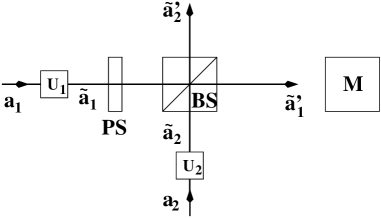
Figure 2: Modified experimental set-up to measure the remaining invariant $J_{4}$ of a two-mode Gaussian state. After the local unitary transformations $U_{1}$ and $U_{2}$, affecting modes $1$ and $2$, respectively, the scheme is identical to the one given in Fig. 1.

The unitary transformations $U_{1}$ and $U_{2}$ are chosen such that the covariance matrix describing the output modes $\tilde{a}_{1}$ and $\tilde{a}_{2}$ is in its standard form $\tilde{V}$ (See Eq. (6)). These unitary transformations preserve the Gaussian character of the input state and they are equivalent to local symplectic transformations $S_{1}$ and $S_{2}$ on $V$. We should bear in mind that the correct transformation is dependent on the one-mode covariance matrices $V_{1}$ and $V_{2}$, which fortunately can be determined locally by standard homodyne detection. Moreover, the important point here is that $S_{1}$ and $S_{2}$ (or $U_{1}$ and $U_{2}$) always exist and that they are local symplectic transformations. In the Appendix we show how to express these transformations as a function of the input local covariance matrices $V_{1}$ and $V_{2}$.

In the standard form $\tilde{V}$ a direct calculation shows that the fourth invariant is given as

$$J_{4}=2\tilde{n}_{1}\tilde{n}_{2}\left(|\tilde{m}_{s}|^{2}+|\tilde{m}_{c}|^{2}\right).$$ (15)

Our task then reduces to the determination of $\tilde{n}_{1}$, $\tilde{n}_{2}$, $|\tilde{m}_{s}|^{2}$, and $|\tilde{m}_{c}|^{2}$ measuring only the output mode $\tilde{a}^{\prime}_{1}$, the one obtained after $\tilde{a_{1}}$ and $\tilde{a_{2}}$ enter the beam splitter.

We first note that $\tilde{n}_{1}$ and $\tilde{n}_{2}$ are trivially related to invariants already measured in the previous scheme: $\tilde{n}_{1}=\sqrt{J_{1}}$ and $\tilde{n}_{2}=\sqrt{J_{2}}$. Second, $J_{3}=|\tilde{m}_{s}|^{2}-|\tilde{m}_{c}|^{2}$ is also known, implying that we just need to measure either $|\tilde{m}_{s}|^{2}$ or $|\tilde{m}_{c}|^{2}$ to obtain $J_{4}$. Analyzing $\tilde{V}_{1}$ we see that,

$$|m_{c}|^{2} = \left[\tilde{N}^{\prime}_{1}\left(\frac{\pi}{4},0\right)\right]^{2}-\tilde{J}^{\prime}_{1}\left(\frac{\pi}{4},0\right),$$ (16)

$$\mbox{Re}\left(\tilde{m}_{s}\right) = \frac{\tilde{n}_{1}+\tilde{n}_{2}}{2}-\tilde{N}^{\prime}_{1}\left(\frac{\pi}{4},0\right),$$ (17)

$$\mbox{Im}\left(\tilde{m}_{s}\right) = \frac{\tilde{n}_{1}+\tilde{n}_{2}}{2}-\tilde{N}^{\prime}_{1}\left(\frac{\pi}{4},\frac{\pi}{2}\right),$$ (18)

where $\tilde{J}^{\prime}_{1}(\theta,\varphi)=\mbox{det}(\tilde{V}^{\prime}_{1})$ and $\tilde{N}^{\prime}_{1}(\theta,\varphi)=\langle(\tilde{a}^{\prime})_{1}^{\dagger}\tilde{a}^{\prime}_{1}+1/2\rangle$ is mode $\tilde{a}^{\prime}_{1}$ average photon number, all quantities determined for a given set of parameters $\theta$ and $\varphi$. Note that although in the standard form (6) the matrix elements $m_{s}$ and $m_{c}$ are real, we have assumed them to be complex, which simplifies the unitary operations $U_{1}$ and $U_{2}$ necessary to transform $V$ to $\tilde{V}$. See the Appendix for more details.

Looking at Eqs. (16)-(18) we see that, similar to the first scheme, only two types of measurements are needed to determine $J_{4}$, namely $\tilde{J}^{\prime}_{1}(\theta,\varphi)$ and $\tilde{N}^{\prime}_{1}(\theta,\varphi)$.

Additionally, the scheme just presented can be employed without relying on the first one. Indeed, assuming that we are always dealing with an experimental set-up as depicted in Fig. 2, the first two invariants are

$$J_{1}=\tilde{n}_{1}^{2} = \left[\tilde{N}^{\prime}_{1}(0,0)\right]^{2},$$ (19)

$$J_{2}=\tilde{n}_{2}^{2} = \left[\tilde{N}^{\prime}_{1}\left(\frac{\pi}{2},0\right)\right]^{2}.$$ (20)

With the aid of Eqs. (16)-(18), the last two invariants, $J_{3}$ and $J_{4}$, are readily obtained.

In summary, given a general two-mode Gaussian state the first scheme allows us to determine the first three invariants ($J_{1},J_{2}$, and $J_{3}$) while the second scheme gives us the fourth as well as the other three invariants. With these four invariants the entanglement content of a two-mode Gaussian state is fully determined.

5 Experimental feasibility

Our last task is to explain how $J^{\prime}_{1}$ and $N^{\prime}_{1}$ (or equivalently $\tilde{J}^{\prime}_{1}$ and $\tilde{N}^{\prime}_{1}$ ) are obtained from experimentally measurable quantities. Firstly, $N^{\prime}_{1}$ is simply the output mode $a^{\prime}_{1}$ photon number (or intensity) and can be easily determined by a photodetection process. The determinant $J^{\prime}_{1}$, on the other hand, is connected to the purity of mode $a^{\prime}_{1}$ by the following expression [16, 17]: $Tr\{(\rho^{\prime}_{1})^{2}\}=1/(2\sqrt{J^{\prime}_{1}})$. Moreover, one can prove that [2] $W(0)=1/(2\pi\sqrt{J^{\prime}_{1}})$ where $W(0)$ is the Wigner function of mode $a^{\prime}_{1}$ at the origin of the phase space. Therefore, any technique developed to measure the purity and/or $W(0)$ can be employed to determine $J^{\prime}_{1}$. Two interesting proposals were presented in Refs. [30, 18]. The first one [30], implemented in Ref. [31], shows that the photon counting statistics allows one to obtain $W(0)$ without any sophisticated data processing. The second one [18], implemented in Ref. [32], employs only a tunable beam splitter and a single-photon detector to obtain the purity of mode $a^{\prime}_{1}$. Remark that both schemes do not require homodyne detection and permit a direct access to $N^{\prime}_{1}$ as well. However, homodyne detection [33] can also be employed for each set of the parameters $\theta$ and $\varphi$ to reconstruct the output mode $a^{\prime}_{1}$ covariance matrix, and thus leading to the immediate calculation of $J^{\prime}_{1}$ and $N^{\prime}_{1}$. Nevertheless, a complete single-mode reconstruction is more than we need to fully characterize the entanglement of a two-mode Gaussian state and also more experimentally demanding than the previous two techniques.

In fact what determines the detection scheme to be employed is the specific scheme detection efficiency in the light frequency range and intensity in use. Obviously a photon counting scheme for the measurement of the Wigner function at the origin of the phase space is more appropriate for low intensity light fields. On the other hand, homodyne reconstruction is more appropriate for continuous bright light fields, unless an alternative procedure allowing access to the photon statistics is implemented, such as for pulsed fields detected by on/off avalanche photodetectors [34]. Photon counting (implemented via avalanche devices with saturated gain where each photon produces a detectable signal (current) at the output) can also be simulated by dual-homodyne schemes [35]. Such schemes may be useful in infrared and optical frequencies since the present day avalanche photodiodes possess very low efficiencies at such communication frequencies [35].

Whichever the scheme employed imperfect detection and signal losses blur the measurement outcomes avoiding an exact determination of the invariants as delineated above. However, in any situation here considered, the losses can be modeled by a beam splitter of transmittance $\eta$ followed by an ideal detector, being $\eta$ attributed to the overall efficiency of the detection scheme [32]. Thus, the actual measured quantities can be corrected by an appropriate rescaling. Firstly, for homodyne detection the procedure to measure the detection efficiency $\eta_{hom}$ is well established from squeezing experiments [36, 32]. Since $J^{\prime}_{1}=I^{\prime}_{1}/4=\left(V^{\prime}_{1,min}V^{\prime}_{1,max}\right)/4$ and $N^{\prime}_{1}=\left(V^{\prime}_{1,min}+V^{\prime}_{1,max}\right)/2$, where $V^{\prime}_{1,min}$ and $V^{\prime}_{1,max}$ are the squeezed and anti-squeezed quadratures variances, respectively, one can show that in terms of the actual measured variances ${\cal V}^{\prime}_{1,min}$ and ${\cal V}^{\prime}_{1,max}$ they are corrected to $V^{\prime}_{1,min}=\left({\cal V}^{\prime}_{1,min}-1+\eta_{hom}\right)/\eta_{hom}$ and $V^{\prime}_{1,max}=\left({\cal V}^{\prime}_{1,max}-1+\eta_{hom}\right)/\eta_{hom}$ [32]. Secondly, the determination of $J^{\prime}_{1}$ and $N^{\prime}_{1}$ via photocounting techniques relies on single photon detection of output mode 1 (given by $a^{\prime}_{1}$) after the two input modes are recombined in a beam splitter of transmittance $T=\cos\theta$. The detector efficiency $\eta$ is modeled by a beam splitter of transmittance $\eta$ followed by an ideal detector, which in Refs. [18, 32] responds with only two measurement outcomes, while in Refs. [30, 31] is a number resolving photodetector. In either case the effects of non-ideal detection can be simply taken into account by substituting $T\rightarrow\eta T$, whose overall effect is to rescale the proper transmittance necessary to obtain all the invariants

6 Conclusion

We have shown that continuous variable entanglement can be directly detected and quantified with few simple measurements. In particular, we have proposed an experimental scheme in which only two types of measurements, i.e. purity (Wigner function at the origin of the phase space) and photon number of a single-mode, are required to characterize the entanglement of a two-mode Gaussian state. Our proposal is valid for either pure or mixed states as well as for either symmetric or non-symmetric Gaussian states, giving always the exact value of the state’s amount of entanglement. Furthermore, our scheme can also be seen as a simple procedure to obtain all the four independent symplectic invariants of a covariance matrix. This allows one to easily test for the existence of entanglement even in non-Gaussian states via the Simon’s sufficient condition of inseparability. Finally we remark that the same scheme could be appropriately adapted for analyzing continuous variable entanglement in other systems than light fields, such as for the motional degrees of freedom of trapped ions [37], or even for Bose-Einstein condensates [38]. This is the case whenever similar processes to the beam splitter and the phase shifter operations can be applied and whenever proper local projective measurements or local state reconstruction can be implemented.

Note: After completion of this manuscript we devised a fully local procedure by which we can measure the four invariants of a general two-mode Gaussian state [39]. Contrary to the schemes here presented, in Ref. [39] there is no need for a non-local unitary operation (as given here by the beam splitter). The trade-off is the inclusion of a classical communication channel and one-mode parity measurements.

Appendix A Obtaining the standard form $\tilde{V}$

The covariance matrix $V$ is generally written as:

$$V=\left(\begin{array}[]{cc}V_{1}&C_{V}\\ C_{V}^{\dagger}&V_{2}\end{array}\right) = \left(\begin{array}[]{cccc}n_{1}&m_{1}&m_{s}&m_{c}\\ m_{1}^{*}&n_{1}&m_{c}^{*}&m_{s}^{*}\\ m_{s}^{*}&m_{c}&n_{2}&m_{2}\\ m_{c}^{*}&m_{s}&m_{2}^{*}&n_{2}\end{array}\right),$$ (27)

where $V_{j}$, $j=1,2$, and $C_{V}$ are block matrices of dimension two. Unitary local operations preserving the Gaussian character of a state described by $V$ are mapped to the following local symplectic transformation [40]:

$$S=\left(\begin{array}[]{cc}S_{1}&0\\ 0&S_{2}\end{array}\right),$$ (28)

where $S_{j}$, $j=1,2$, is given as

$$S_{j}=\left(\begin{array}[]{cc}\mathrm{e}^{-i\alpha_{j}}\cosh\theta_{j}&\mathrm{e}^{i\beta_{j}}\sinh\theta_{j}\\ \mathrm{e}^{-i\beta_{j}}\sinh\theta_{j}&\mathrm{e}^{i\alpha_{j}}\cosh\theta_{j}\end{array}\right),$$ (29)

with $\alpha_{j}$, $\beta_{j}$, and $\theta_{j}$ real parameters. The first one is related to rotations of the quadratures of the quantized electromagnetic field and the last one to local squeezing operations. The new covariance matrix $\tilde{V}$ is connected to $V$ by the following relation [40, 41],

$$\tilde{V}=SVS^{\dagger},$$ (30)

which implies that

$$\tilde{V}_{j} = S_{j}V_{j}S_{j}^{\dagger},$$ (31)

$$\tilde{C}_{V} = S_{1}C_{V}S_{2}^{\dagger}.$$ (32)

Explicitly, Eq. (31) gives for the non-diagonal term of $\tilde{V}_{j}$:

$$\tilde{m}_{j} = \mathrm{e}^{-2\mathrm{i}\alpha_{j}}m_{j}\cosh^{2}\theta_{j}+\mathrm{e}^{2\mathrm{i}\beta_{j}}m_{j}^{*}\sinh^{2}\theta_{j}$$ (33)

$$+\mathrm{e}^{\mathrm{i}(\beta_{j}-\alpha_{j})}n_{j}\sinh(2\theta_{j}).$$

By setting $m_{j}=|m_{j}|\mathrm{e}^{\mathrm{i}\mu_{j}}$ and solving for $\tilde{m}_{j}=0$ we get

$$\alpha_{j}=\beta_{j}=\frac{\mu_{j}+\pi}{2},$$ (34)

$$\tanh(2\theta_{j})=\frac{|m_{j}|}{n_{j}}.$$ (35)

Note that this is one of several other solutions. However, for our purposes, one is enough to prove that $V$ can be locally transformed to $\tilde{V}$.

References

- [1] C. H. Bennett and D. P. DiVincenzo, Nature (London) 404, 247 (2000).
- [2] S.L. Braunstein and P. van Loock, Rev. Mod. Phys. 77, 513 (2005).
- [3] G. Adesso and F. Illuminati, J. Physics A: Math. Theor. 40, 7821 (2007).
- [4] J. Eisert and M. B. Plenio, Int. J. Quant. Inf. 1, 479 (2003).
- [5] A. K. Ekert, Phys. Rev. Lett. 67, 661 (1991).
- [6] O. Cohen, Helv. Phys. Acta 70, 710 (1997).
- [7] S. F. Pereira, Z. Y. Ou and H. J. Kimble, Phys. Rev. A 62, 042311 (2000).
- [8] C. H. Bennett and S. J. Wiesner, Phys. Rev. Lett. 69, 2881 (1992).
- [9] M. Ban, J. Opt. B: Quantum Semiclass. Opt. 1, L9 (1999).
- [10] S. L. Braunstein and H. J. Kimble, Phys. Rev. A 61 042302 (2000).
- [11] C. H. Bennett et al., Phys. Rev. Lett. 70, 1895 (1993).
- [12] L. Vaidman, Phys. Rev. A 49, 1473 (1994).
- [13] S. L. Braunstein and H. J. Kimble, Phys. Rev. Lett. 80, 869 (1998).
- [14] F. Mintert, M. Kuś, and A. Buchleitner, Phys. Rev. Lett. 95, 260502 (2005).
- [15] S. P. Walborn, P. H. Souto Ribeiro, L. Davidovich, F. Mintert, and A. Buchleitner, Nature (London) 440, 1022 (2006).
- [16] G. Adesso, A. Serafini, and F. Illuminati, Phys. Rev. Lett. 92, 087901 (2004).
- [17] G. Adesso, A. Serafini, and F. Illuminati, Phys. Rev. A 70, 022318 (2004).
- [18] J. Fiurášek and N. J. Cerf, Phys. Rev. Lett, 93, 063601 (2004).
- [19] V. Josse, A. Dantan, A. Bramati, M. Pinard, and E. Giacobino, Phys. Rev. Lett. 92, 123601 (2004).
- [20] G. Vidal and R. F. Werner, Phys. Rev. A 65, 032314 (2002).
- [21] G. Giedke, M. M. Wolf, O. Krüger, R. F. Werner, and J. I. Cirac, Phys. Rev. Lett. 91, 107901 (2003).
- [22] R. Simon, Phys. Rev. Lett. 84, 2726 (2000).
- [23] From now on we assume since the first moments does not affect the entanglement content of a CV-state and can locally be set to zero by a displacement of the and quadratures.
- [24] G. Rigolin and C. O. Escobar, Phys. Rev. A 69, 012307 (2004).
- [25] We call the covariance matrix for the creation and annihilation operators while is the covariance matrix of the quadratures of the electromagnetic field.
- [26] M. C. de Oliveira, Phys. Rev. A 72, 012317 (2005).
- [27] Note that since we assumed we also have .
- [28] Starting with the standard form of one can easily see that can be brought to (6) by expressing it as a function of the matrix elements .
- [29] V. D’Auria, A. Porzio, S. Solimeno, S. Olivares, and M. G. A. Paris, J. Opt. B: Quantum Semiclass. Opt. 7, S750 (2005).
- [30] K. Banaszek and K. Wódkiewicz, Phys. Rev. Lett. 76, 4344 (1996).
- [31] K. Banaszek, C. Radzewicz, K. Wódkiewicz, and J. S. Krasinski, Phys. Rev. A 60, 674 (1999).
- [32] J. Wenger, J. Fiurášek, R. Tualle-Brouri, N. J. Cerf, and P. Grangier, Phys. Rev. A 70, 053812 (2004).
- [33] A. Ourjoumtsev, R. Tualle-Brouri, and P. Grangier, Phys. Rev. Lett. 96, 213601 (2006).
- [34] G. Zambra et al., Phys. Rev. Lett. 95, 063602 (2005).
- [35] K. Nemoto and S. L. Braunstein, Phys. Rev. A 66, 032306 (2002).
- [36] R. E. Slusher, P. Grangier, A. LaPorta, B. Yurke, and M. J. Potasek, Phys. Rev. Lett. 59, 2566 (1987).
- [37] D. Leibfried et al., Phys. Rev. Lett. 77 4281 (1996).
- [38] B. R. da Cunha and M. C. de Oliveira, Phys. Rev. A 75, 063615 (2007).
- [39] L. F. Haruna, M. C. de Oliveira, and G. Rigolin, Phys. Rev. Lett. 98, 150501 (2007); ibidem 99, 059902(E) (2007).
- [40] R. Simon, N. Mukunda, and B. Dutta, Phys. Rev. A 49, 1567 (1994).
- [41] M. C. de Oliveira, Phys. Rev. A, 70, 034303 (2004).