Operational approach to the Uhlmann holonomy

Abstract

We suggest a physical interpretation of the Uhlmann amplitude of a density operator. Given this interpretation we propose an operational approach to obtain the Uhlmann condition for parallelity. This allows us to realize parallel transport along a sequence of density operators by an iterative preparation procedure. At the final step the resulting Uhlmann holonomy can be determined via interferometric measurements.

I Introduction

If a quantum system depends on a slowly varying external parameter, Berry berry84 showed that there is a geometric phase factor associated to the path that an eigenvector of the corresponding Hamiltonian traverses during the evolution. These geometric phase factors were later generalized by Wilczek and Zee wilczek84 to holonomies, i.e., unitary state changes associated with the motion of a degenerate subspace of the parameter-dependent Hamiltonian. In view of the Berry phase and Wilczek-Zee holonomy, one may ask if a phase or a holonomy can be associated with families of mixed states. This was answered in the affirmative by Uhlmann Uhl by introducing “amplitudes” of density operators, and a condition for parallelity of amplitudes along a family of density operators (for other approaches to geometric phases and holonomies of mixed states and their relation to the Uhlmann approach, see Refs. Ell ; ME2 ; Sjo ; Pei ; Tong ; Cha ; Sar ; Slater ; ME ; rezakhani06 ).

As mentioned above, the Berry phases and the non-Abelian holonomies can be given a clear physical and operational interpretation in terms of the evolution caused by adiabatically evolving quantum systems. One may also consider the evolution as caused by a sequence of projective measurements of observables with nondegenerate or degenerate eigenvalues, giving rise to a Berry phase or a non-Abelian holonomy, respectively. The physical interpretation of the Uhlmann amplitudes and their parallel transport is less clear. One interpretation of the Uhlmann amplitude Uhl2 ; Dittmann ; ME ; tidstrom03 ; rezakhani06 is that it corresponds to the state vector of a purification on a combined system and ancilla. Here we suggest another interpretation, where the amplitude corresponds to an “off-diagonal block” of a density operator with respect to two orthogonal subspaces. In this framework, we address the question of how to obtain an explicitly operational approach to the Uhlmann holonomy, which, to the knowledge of the authors, has not been previously considered comment1 ; sjoqvist06 ; uhlmann91 .

The structure of the paper is as follows. In Sec. II we give a brief introduction to the Uhlmann holonomy. In Sec. III we introduce our interpretation of the Uhlmann amplitude and show that it is possible to determine the amplitude using an interferometric approach. Given the interpretation of the amplitude we consider an operational implementation of the parallelity condition in Sec. IV.1, and in Sec. IV.2 we use the parallelity condition to establish the parallel transport. In Sec. V we present a technique to generate the states needed in the parallel transport procedure. We generalize the approach to sequences of not faithful density operators (operators not of full rank) and introduce a preparation procedure for the density operators needed in the generalized case in Sec. VI. The paper ends with the conclusions in Sec. VII.

II Uhlmann holonomy

Consider a sequence of density operators $\sigma_{1},\sigma_{2},\ldots,\sigma_{K}$ on a Hilbert space $\mathcal{H}_{I}$. A sequence of amplitudes of these states are operators $W_{1},W_{2},\ldots,W_{K}$ on $\mathcal{H}_{I}$, such that $\sigma_{k}=W_{k}W_{k}^{\dagger}$. In Uhlmann’s terminology Uhl , a density operator $\sigma$ is faithful if its range $\mathcal{R}(\sigma)$ coincides with the whole Hilbert space, i.e., if $\mathcal{R}(\sigma)=\mathcal{H}_{I}$ (Note that what we refer to as a faithful operator is often referred to as an operator of “full rank”.) For the present we shall assume that all density operators are faithful, and return to the question of unfaithful operators in Sec. VI. Using the polar decomposition LanTis the amplitudes can be written $W_{k}=\sqrt{\sigma_{k}}V_{k}$, where $V_{k}$ is unitary. The gauge-freedom in the Uhlmann approach is the freedom to choose the unitary operators $V_{k}$. For faithful density operators $\sigma_{k}$ adjacent amplitudes are parallel if and only if $W_{k+1}^{\dagger}W_{k}>0$. Given an initial amplitude $W_{1}$ and the corresponding unitary operator $V_{1}$, the parallelity condition uniquely determines the sequence of amplitudes $W_{1},W_{2},\ldots,W_{K}$, and unitaries $V_{1},V_{2},\ldots,V_{K}$. The Uhlmann holonomy of the sequence of density operators is defined as $U_{\textrm{Uhl}}=V_{K}V_{1}^{\dagger}$ comment2 .

The Uhlmann approach fits naturally within the framework of differential geometry. The amplitudes are the elements of the total space of the fiber bundle, with the set of faithful density operators as the base manifold, and the set of unitary operators $U(N)$ as the fibers. Moreover, $WW^{\dagger}=\sigma$ gives the projection from the total space down to the base manifold. Finally, given a sequence in the base manifold of density operators, the parallelity condition $W_{k+1}^{\dagger}W_{k}>0$ induces a unique sequence in the total space, leading to an element of the fiber as the resulting holonomy.

III Interpretation of the Uhlmann amplitude

As mentioned above, our first task is to find a physically meaningful interpretation of the Uhlmann amplitude. We regard the density operators in the given sequence as operators on a Hilbert space $\mathcal{H}_{I}$ of finite dimension $N$. In addition, we append a single qubit with Hilbert space $\mathcal{H}_{s}={\textrm{Sp}}\{|0\rangle,|1\rangle\}$, with $|0\rangle$ and $|1\rangle$ orthonormal, and where Sp denotes the linear span. The total Hilbert space we denote $\mathcal{H}=\mathcal{H}_{I}\otimes\mathcal{H}_{s}$. Note that $\mathcal{H}$ can be regarded as the state space of a single particle in the two paths of a Mach-Zehnder interferometer, where $\mathcal{H}_{I}$ corresponds to the internal degrees of freedom (e.g., spin or polarization) of the particle and $|0\rangle$ and $|1\rangle$ correspond to the two paths.

We let $\mathbb{Q}(\sigma^{(0)},\sigma^{(1)})$ denote the set of density operators $\rho$ on $\mathcal{H}=\mathcal{H}_{I}\otimes\mathcal{H}_{s}$ such that

$$\langle 0|\rho|0\rangle=\frac{1}{2}\sigma^{(0)},\quad\langle 1|\rho|1\rangle=\frac{1}{2}\sigma^{(1)},$$ (1)

i.e., $\mathbb{Q}(\sigma^{(0)},\sigma^{(1)})$ consists of those states that have the prescribed “marginal states” $\sigma_{0}$ and $\sigma_{1}$, each found with probability one half. We span $\mathbb{Q}(\sigma^{(0)},\sigma^{(1)})$ by varying the “off-diagonal” operator $\langle 0|\rho|1\rangle$. What freedom do we have in the choice of the operator $\langle 0|\rho|1\rangle$? This question turns out to have the following answer.

Proposition 1.

$\rho\in\mathbb{Q}(\sigma^{(0)},\sigma^{(1)})$ if and only if there exists an operator $\widetilde{V}$ on $\mathcal{H}_{I}$ such that

$$\rho = \frac{1}{2}\sigma^{(0)}\otimes|0\rangle\langle 0|+\frac{1}{2}\sigma^{(1)}\otimes|1\rangle\langle 1|$$ (2)

$$+\frac{1}{2}\sqrt{\sigma^{(0)}}\widetilde{V}\sqrt{\sigma^{(1)}}\otimes|0\rangle\langle 1|$$

$$+\frac{1}{2}\sqrt{\sigma^{(1)}}\widetilde{V}^{\dagger}\sqrt{\sigma^{(0)}}\otimes|1\rangle\langle 0|,$$

and

$$\widetilde{V}\widetilde{V}^{\dagger}\leq\hat{1}_{I}.$$ (3)

To prove this we use the following (see Lemma 13 in Ref. Ann ): Let $A$, $B$, and $C$ be operators on $\mathcal{H}_{I}$, and let $A\geq 0$, $B\geq 0$, and

$$F=A\otimes|0\rangle\langle 0|+C\otimes|0\rangle\langle 1|+C^{\dagger}\otimes|1\rangle\langle 0|+B\otimes|1\rangle\langle 1|.$$ (4)

Then $F$ is positive semidefinite if and only if

$$P_{\mathcal{R}(A)}CP_{\mathcal{R}(B)}=C,\quad A\geq CB^{\ominus}C^{\dagger},$$ (5)

where $P_{\mathcal{R}(A)}$ and $P_{\mathcal{R}(B)}$ denote the projectors onto the ranges $\mathcal{R}(A)$ and $\mathcal{R}(B)$ of $A$ and $B$, respectively. In Eq. (5) the symbol $B^{\ominus}$ denotes the Moore-Penrose (MP) pseudo inverse LanTis of $B$. The reason why the MP inverse is used is to allow us to handle those cases when $A$ and $B$ have ranges that are proper subspaces of $\mathcal{H}_{I}$. Note that when $B$ is invertible, the MP inverse coincides with the ordinary inverse.

To prove Proposition 1 we first note that if $\rho$ can be written as in Eq. (2), then ${\textrm{Tr}}(\rho)=1$ and $\rho$ satisfies Eq. (1). If we compare Eqs. (2) and (4), we can identify $A$, $B$, and $C$, and see that they satisfy the conditions in Eq. (5). From this follows that $\rho$ is positive semidefinite. We can thus conclude that $\rho$ is a density operator and an element of $\mathbb{Q}(\sigma^{(0)},\sigma^{(1)})$.

Now, we wish to show the converse, i.e., if $\rho\in\mathbb{Q}(\sigma^{(0)},\sigma^{(1)})$ then it can be written as in Eq. (2). By definition it follows that we can identify $A=\sigma^{(0)}/2$ and $B=\sigma^{(1)}/2$ in Eq. (4). Since $\rho$ is positive semidefinite it follows that $C$ has to satisfy the conditions in Eq. (5) and thus

$$\frac{1}{2}\sigma^{(0)}\geq 2C{\sigma^{(1)}}^{\ominus}C^{\dagger}.$$ (6)

Define $\widetilde{V}=2\sqrt{\sigma^{(0)}}^{\ominus}C\sqrt{\sigma^{(1)}}^{\ominus}$. From Eq. (6) it follows that $\widetilde{V}$ satisfies $\widetilde{V}\widetilde{V}^{\dagger}\leq 1$. Moreover,

$$\frac{1}{2}\sqrt{\sigma^{(0)}}\widetilde{V}\sqrt{\sigma^{(1)}}=P_{\mathcal{R}(\sigma^{(0)})}CP_{\mathcal{R}(\sigma^{(1)})}=C,$$ (7)

where the last equality follows from Eq. (5). Thus we have shown that $\rho\in\mathbb{Q}(\sigma^{(0)},\sigma^{(1)})$ if and only if $\rho$ can be written as in Eq. (2). This proves Proposition 1.

Now, consider the set of density operators $\mathbb{Q}(\sigma,\hat{1}_{I}/N)$, i.e., when one of the marginal states is the maximally mixed state. According to Eq. (2) it follows that $\langle 0|\rho|1\rangle=\sqrt{\sigma}\widetilde{V}/(2\sqrt{N})$. Note that the condition in Eq. (3) allows us to choose $\widetilde{V}$ as an arbitrary unitary operator, and we thus obtain

$$\rho\equiv\mathcal{D}(\sigma,W) = \frac{1}{2}\sigma\otimes|0\rangle\langle 0|+\frac{1}{2N}\hat{1}_{I}\otimes|1\rangle\langle 1|$$

$$+\frac{1}{2\sqrt{N}}W\otimes|0\rangle\langle 1|+\frac{1}{2\sqrt{N}}W^{\dagger}\otimes|1\rangle\langle 0|,$$

where $W$ is an arbitrary Uhlmann amplitude of the density operator $\sigma$, i.e., $\sigma=WW^{\dagger}$. We thus have a physical realization of the Uhlmann amplitude as corresponding to the off-diagonal operator $\langle 0|\rho|1\rangle$. Note that $\mathbb{Q}(\sigma,\hat{1}_{I}/N)$ contains more states than those corresponding to amplitudes of $\sigma$. As will be seen later, these other states have an important role when we consider sequences of density operators that are not faithful.

Let us note some of the differences between the above interpretation of the Uhlmann amplitude and the interpretation in terms of purifications Uhl2 ; Dittmann ; ME ; tidstrom03 ; rezakhani06 . In the latter, the amplitude corresponds to a pure state on a combination of the system and an ancilla, such that the density operator $\sigma$ is retained when the ancilla is traced over. Similarly as for the purification interpretation, we consider here an extension to a larger Hilbert space, but in a different manner. In the purification approach we extend the Hilbert space as $\mathcal{H}_{I}\otimes\mathcal{H}_{I}$, while in the present approach we extend the space as $\mathcal{H}_{I}\otimes\mathcal{H}_{s}$ comment3 . Since $\mathcal{H}_{s}$ is two-dimensional it follows that $\mathcal{H}_{I}\otimes\mathcal{H}_{s}\simeq\mathcal{H}_{I}\oplus\mathcal{H}_{I}$ , i.e., the space we use to represent the state and its amplitude is isomorphic to an orthogonal sum of two copies of $\mathcal{H}_{I}$ (one for each path of the interferometer). With respect to these two subspaces the amplitude is essentially carried by the off-diagonal operator, rather than the whole density operator $\mathcal{D}(\sigma,W)$. In some sense the amplitude describes the nature of the superposition between these two subspaces, or equivalently, the coherence of the particle between the two paths of the interferometer. One can also note from Eq. (III) that the total state $\mathcal{D}(\sigma,W)$ is mixed rather than pure in general. Note that this subspace approach is closely related to the investigations of channels and interferometry in Refs. Ann ; Oi ; JA ; OiJA . Let us finally point out that the subspace approach gives a more compact representation than the purification approach (if $\dim(\mathcal{H}_{I})>2$ and $\sigma$ is full rank), in the sense that in the former case a single qubit is added to the system, while for latter we have to add a whole copy of the original system.

Determining the amplitude.

Given a state $\rho=\mathcal{D}(\sigma,W)$ the unitary part $V$ of the amplitude $W=\sqrt{\sigma}V$ can be experimentally determined by first applying onto $\rho$ the unitary operation

$$U_{tot}=\hat{1}_{I}\otimes|0\rangle\langle 0|+U\otimes|1\rangle\langle 1|,$$ (9)

where $U$ is a variable unitary operator on $\mathcal{H}_{I}$. Next, a Hadamard gate is applied onto $\mathcal{H}_{s}$, followed by a measurement to determine the probability $p$ to find the state $|0\rangle\langle 0|$. This probability turns out to be

$$p=\frac{1}{2}+\frac{1}{2\sqrt{N}}{\textrm{Re}}{\textrm{Tr}}(\sqrt{\sigma}VU^{\dagger}).$$ (10)

By varying $U$ until $p$ is maximized we determine $U=V$ uniquely, if $\sigma$ is faithful. Thus, $V$ can be operationally defined as the unitary operator giving the largest detection probability in this setup, indirectly determining the amplitude $W=\sqrt{\sigma}V$.

IV Realization of the Uhlmann holonomy

IV.1 Parallelity

Here, we address the question of implementing the parallelity condition between two amplitudes. Consider two faithful density operators $\sigma_{a}$ and $\sigma_{b}$. As mentioned above the corresponding amplitudes are parallel if and only if $W_{b}^{\dagger}W_{a}>0$. Let $\{|\chi_{k}\rangle\}_{k}$ be an arbitrary orthonormal basis of $\mathcal{H}_{I}$. We denote $|\chi_{k},x\rangle=|\chi_{k}\rangle|x\rangle$ and $P_{x}=\hat{1}_{I}\otimes|x\rangle\langle x|$ for $x=0,1$. Since we use the Hilbert space $\mathcal{H}=\mathcal{H}_{I}\otimes\mathcal{H}_{s}$ to represent a density operator and its amplitude, we consider two copies of $\mathcal{H}$ in order to compare the amplitudes of two different density operators. On $\mathcal{H}\otimes\mathcal{H}$ we define the following unitary and Hermitian operator:

$$Z = \sum_{kl}|\chi_{k},0\rangle\langle\chi_{l},1|\otimes|\chi_{l},1\rangle\langle\chi_{k},0|$$ (11)

$$+\sum_{kl}|\chi_{l},1\rangle\langle\chi_{k},0|\otimes|\chi_{k},0\rangle\langle\chi_{l},1|$$

$$+P_{0}\otimes P_{0}+P_{1}\otimes P_{1}.$$

For $\rho_{a}=\mathcal{D}(\sigma_{a},W_{a})$ and $\rho_{b}=\mathcal{D}(\sigma_{b},W_{b})$,

$$E = {\textrm{Tr}}(Z\rho_{b}\otimes\rho_{a})$$ (12)

$$= \frac{1}{2}+\frac{1}{2N}{\textrm{Re}}{\textrm{Tr}}(W_{b}^{\dagger}W_{a}).$$

This means that the maximal value of the real and non-negative quantity $E$ is reached when $W_{b}$ is parallel to $W_{a}$.

Now we use the fact that $Z$ is a unitary operator in order to test the degree of parallelity between two amplitudes (see Fig. 1). Consider an “extra” qubit $e$ whose Hilbert space $\mathcal{H}_{e}$ is spanned by the orthonormal basis $\{|0_{e}\rangle,|1_{e}\rangle\}$ (not to be confused with $\mathcal{H}_{s}$ and the corresponding qubit in the construction of $\mathcal{D}(\sigma,W)$). We first prepare the state $|0_{e}\rangle\langle 0_{e}|\otimes\rho_{b}\otimes\rho_{a}$ on the total Hilbert space $\mathcal{H}_{e}\otimes\mathcal{H}\otimes\mathcal{H}=\mathcal{H}_{e}\otimes\mathcal{H}_{I}\otimes\mathcal{H}_{s}\otimes\mathcal{H}_{I}\otimes\mathcal{H}_{s}$. We apply a Hadamard gate on qubit $e$, followed by an application of the unitary operation

$$U_{Z}=|0_{e}\rangle\langle 0_{e}|\otimes Z+|1_{e}\rangle\langle 1_{e}|\otimes\hat{1}\otimes\hat{1},$$ (13)

i.e., an application of the unitary operation $Z$, conditioned on the qubit $e$. Finally, we apply the Hadamard gate on qubit $e$ and measure the probability to find $e$ in state $|0_{e}\rangle\langle 0_{e}|$ comment4 . This procedure results in the detection probability

$$p=\frac{1}{2}+\frac{1}{2}E=\frac{3}{4}+\frac{1}{4N}{\textrm{Re}}{\textrm{Tr}}(W_{b}^{\dagger}W_{a}).$$ (14)

Thus, the probability $p$ is maximal when $W_{b}$ is parallel to $W_{a}$ in the Uhlmann sense. In other words, given the state $\rho_{a}=\mathcal{D}(\sigma_{a},W_{a})$ we prepare various states $\rho_{b}=\mathcal{D}(\sigma_{b},W_{b})$ until we find the amplitude $W_{b}$ that maximizes the probability $p$ comment6 . We have thus obtained an operational method to find parallel amplitudes. One may note the similarity between this procedure and the method introduced in prod to estimate the trace of products of density operators.

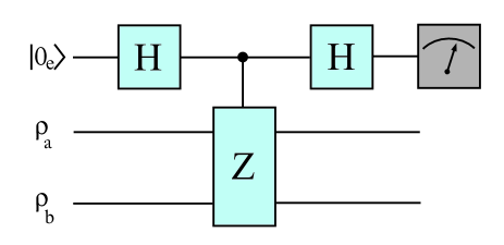
Figure 1: (Color online) The degree of parallelity between the amplitudes $W_{a}$ and $W_{b}$ of the states $\sigma_{a}$ and $\sigma_{b}$, respectively, can be tested by applying this circuit onto the states $\rho_{a}=\mathcal{D}(\sigma_{a},W_{a})$ and $\rho_{b}=\mathcal{D}(\sigma_{b},W_{b})$ defined by Eq. (III). A single “extra” qubit is prepared in state $|0_{e}\rangle$ and a Hadamard gate is applied. Conditional on the $|0_{e}\rangle$ state of the extra qubit, the unitary operation $Z$, defined in Eq. (11), is applied to $\rho_{a}\otimes\rho_{b}$. After the application of a second Hadamard gate on the extra qubit, the degree of parallelity between $W_{a}$ and $W_{b}$ can be inferred from the probability to find the extra qubit in state $|0_{e}\rangle$. Parallelity is obtained when the probability is maximal.

The above approach is based on the fact that $Z$ is a unitary operator and consequently corresponds to a state change. As mentioned above, $Z$ is also Hermitian and can thus be regarded as representing an observable. Thus, one may consider an alternative approach where given the state $\rho_{a}=\mathcal{D}(\sigma_{a},W_{a})$, we prepare states $\rho_{b}=\mathcal{D}(\sigma_{b},W_{b})$ until we find the amplitude $W_{b}$ that results in the maximal expectation value of the observable.

It is worth to point out that the maximization which implements the parallelity condition relates the Uhlmann holonomy with various well known and closely related quantities. We first note that Eqs. (12) and (14) contain ${\textrm{Re}}{\textrm{Tr}}(W_{b}^{\dagger}W_{a})$. When this is maximized over all amplitudes $W_{b}$ of $\sigma_{b}$ we find that $\sup{\textrm{Re}}{\textrm{Tr}}(W_{b}^{\dagger}W_{a})=F(\sigma_{b},\sigma_{a})$, where $F(\sigma_{b},\sigma_{a})={\textrm{Tr}}\sqrt{\sqrt{\sigma_{b}}\sigma_{a}\sqrt{\sigma_{b}}}$ is the quantum fidelity. Closely related is the transition probability $F^{2}(\sigma_{b},\sigma_{a})$ transpr , and the Bures metric $d(\sigma_{a},\sigma_{b})=\sqrt{2-2F^{2}(\sigma_{a},\sigma_{b})}$ Bures ; Arkai that has been proved to be directly related to the Uhlmann holonomy Dittmann .

IV.2 Parallel transport

The procedure to find parallel amplitudes allows us to obtain parallel transport. Suppose we are given a sequence of operators $\sigma_{j}$ on $\mathcal{H}_{I}$ for $j=1,2,\ldots,K$. We wish to construct a sequence $\rho_{j}=\mathcal{D}(\sigma_{j},W_{j})$, such that $W_{j}$ form a parallel transported sequence of Uhlmann amplitudes. Suppose moreover that $\rho_{1}$ is given (in order to fix the initial amplitude $W_{1}$). We can now use the following iterative procedure:

• Prepare $\rho_{k}$.

• Vary the preparations $\rho=\mathcal{D}(\sigma_{k+1},W)$ over all amplitudes $W$ of $\sigma_{k+1}$ until the maximum of ${\textrm{Tr}}(Z\rho\otimes\rho_{k})$ is reached.

• Let $\rho_{k+1}=\rho$.

After the final step $K$ we have prepared the state $\rho_{K}$ containing the amplitude $W_{K}=\sqrt{\sigma_{K}}U_{\textrm{Uhl}}V_{1}$, where $U_{\textrm{Uhl}}$ is the Uhlmann holonomy and $V_{1}$ is the unitary part of the chosen initial amplitude $W_{1}$. The state $\rho_{K}$ can be modified by applying the unitary operator

$$U_{\textrm{mod}}=\hat{1}_{I}\otimes|0\rangle\langle 0|+V_{1}\otimes|1\rangle\langle 1|,$$ (15)

which results in the new state

$$\widetilde{\rho}_{K}=U_{\textrm{mod}}\rho_{K}U_{\textrm{mod}}^{\dagger}=\mathcal{D}(\sigma_{K},\sqrt{\sigma_{K}}U_{\textrm{Uhl}}),$$ (16)

and hence $\langle 0|\widetilde{\rho}_{K}|1\rangle=\sqrt{\sigma_{K}}U_{\textrm{Uhl}}/(2\sqrt{N})$. Given this state we obtain the Uhlmann holonomy $U_{\textrm{Uhl}}$ as the unitary operator that yields the maximal detection probability, as described by Eq. (10).

Although the iterative procedure described above is realizable in principle, it is no doubt the case that it would be challenging in practice, since at each step of the procedure we must implement an optimization to find parallel amplitudes. However, the functions we optimize over have rather favorable properties. In the case of faithful density operators one can show that the function (taken over all amplitudes $W_{b}$) defined by Eq. (14) is such that there is no local maximum except for the global maximum. In the case of not faithful density operators the global maximum is not unique, but any of them gives the desired result, as shown in Sec. VI. Moreover, it still remains the case that every local maximum is a global maximum. Hence, in both the faithful and unfaithful case we can apply local optimization methods (see, e.g., Chong ). The fact that local optimization techniques are applicable is favorable for practical implementations, and improve the chances to find efficient procedures. However, a more detailed analysis would be required to determine what efficiency that ultimately can be obtained. This question is, however, not considered here.

V State preparation

Since the parallel transport procedure involves repeated preparations of states $\mathcal{D}(\sigma,W)$, with arbitrary amplitudes $W$ of $\sigma$, we here consider preparation techniques for such states (see Fig. 2). First, we show how to prepare the state $\rho=\mathcal{D}(\sigma,\sqrt{\sigma})$. Consider the following orthogonal but not normalized vectors:

$$|\psi_{k}\rangle=\sqrt{\lambda_{k}/2}|k\rangle|0\rangle+|k\rangle|1\rangle/\sqrt{2N},$$ (17)

where $\lambda_{k}$ and $|k\rangle$ are eigenvalues and corresponding orthonormal eigenvectors of $\sigma$. One can check that $\sum_{k}|\psi_{k}\rangle\langle\psi_{k}|=\rho$. The probability distribution $(1/N,\ldots,1/N)$ is majorized majo by the vector $(\lambda_{1},\ldots,\lambda_{N})$. Thus, there exists Horn a unitary matrix $\boldsymbol{U}$ such that $\sum_{k}|\boldsymbol{U}_{jk}|^{2}\lambda_{k}=1/N$ for all $j=1,\ldots,N$ (see also Refs. nielsen00 ; rezakhani06 ). Define the vectors

$$|\eta_{j}\rangle=\sqrt{N}\sum_{k}\boldsymbol{U}_{jk}|\psi_{k}\rangle.$$ (18)

One can check that these vectors are normalized. Since $\boldsymbol{U}$ is unitary it follows that $N^{-1}\sum_{j}|\eta_{j}\rangle\langle\eta_{j}|=\rho$. Thus, $\rho$ is the result if we prepare $|\eta_{j}\rangle$ with probability $1/N$. One can check that $\langle\eta_{j}|P_{0}|\eta_{j}\rangle=1/2$. Thus there exist normalized vectors $|\eta_{j}^{0}\rangle,|\eta_{j}^{1}\rangle\in\mathcal{H}_{I}$, such that

$$|\eta_{j}\rangle=\frac{1}{\sqrt{2}}|\eta_{j}^{0}\rangle|0\rangle+\frac{1}{\sqrt{2}}|\eta_{j}^{1}\rangle|1\rangle.$$ (19)

For any normalized $|\eta\rangle\in\mathcal{H}_{I}$ there exist unitary operators $U_{j}^{(0)}$ and $U_{j}^{(1)}$ such that $U_{j}^{(0)}|\eta\rangle=|\eta_{j}^{0}\rangle$ and $U_{j}^{(1)}|\eta\rangle=|\eta_{j}^{1}\rangle$. The state $\rho$ is prepared if we apply a Hadamard gate to the state $|\eta\rangle|0\rangle$, followed by the application of the unitary operator $U_{j}^{(0)}\otimes|0\rangle\langle 0|+U_{j}^{(1)}\otimes|1\rangle\langle 1|$ with probability $p_{j}=1/N$. In terms of an interferometric approach we thus apply a pair of unitary operations $U_{j}^{(0)}$, $U_{j}^{(1)}$, one in each path of the interferometer, with the choice of pair based on the output of a random generator shared between the two paths. This procedure leads to the output density operator $\rho=\mathcal{D}(\sigma,\sqrt{\sigma})$. To obtain a state that corresponds to an arbitrary amplitude, i.e., $\mathcal{D}(\sigma,\sqrt{\sigma}V)$ with $V$ unitary, we just apply the unitary operation $\hat{1}_{I}\otimes|0\rangle\langle 0|+V\otimes|1\rangle\langle 1|$ onto $\rho$.

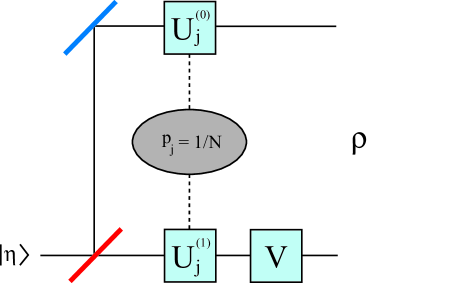
Figure 2: (Color online) Preparation method to obtain the states $\rho=\mathcal{D}(\sigma,W)$ that represent density operators $\sigma$ and their amplitudes $W$, as defined in Eq. (III). The output state $\rho$ describes both the path state and the internal state of the particle. All states $\mathcal{D}(\sigma,W)$ can be prepared by letting a particle in a pure internal reference state $|\eta\rangle$ and path state $|0\rangle$ fall onto a 50-50 beam-splitter, followed by unitary operations acting separately in the two paths on the internal state of the particle. The application of the unitary operations have to be coordinated by a shared output of a random generator, implementing unitary operators $U_{j}^{(0)}$ and $U_{j}^{(1)}$ in respective path, with probability $p_{j}=1/N$. By application of a final unitary $V$ in path $1$ we can obtain any desired amplitude $W=\sqrt{\sigma}V$.

VI Admissible sequences

So far we have assumed that the density operators are faithful. Here we consider the generalization to admissible sequences (defined below) of not faithful density operators Uhl . When the assumption of faithfulness is removed we have to review all the steps in the procedure. First, we note that Eqs. (4) - (III) are true irrespective of whether the involved density operators are faithful or not. By using the polar decompositions

$$\sqrt{\sigma_{k+1}}\sqrt{\sigma_{k}}=\sqrt{\sqrt{\sigma_{k+1}}\sigma_{k}\sqrt{\sigma_{k+1}}}U_{k+1,k},$$ (20)

the Uhlmann holonomy can be reformulated as $U_{\textrm{Uhl}}=U_{K,K-1}\ldots U_{2,1}$ comment2 . If the density operators are not faithful then Eq. (20) does not determine $U_{k+1,k}$ uniquely. However, if we require $U_{k+1,k}$ to be a partial isometry comment8 with initial space $\mathcal{R}(\sqrt{\sigma_{k}}\sqrt{\sigma_{k+1}})$ and final space $\mathcal{R}(\sqrt{\sigma_{k+1}}\sqrt{\sigma_{k}})$, then Eq. (20) uniquely determines $U_{k+1,k}$ to be the partial isometry

$$U_{k+1,k}=\sqrt{\sqrt{\sigma_{k+1}}\sigma_{k}\sqrt{\sigma_{k+1}}}^{\ominus}\sqrt{\sigma_{k+1}}\sqrt{\sigma_{k}}.$$ (21)

If the sequence of density operators is such that the final space of $U_{k+1,k}$ matches the initial space of $U_{k+2,k+1}$, then we may define the Uhlmann holonomy as the partial isometry $U_{\textrm{Uhl}}=U_{K,K-1}\ldots U_{2,1}$ Uhl . A sequence of density operators that results in such matched initial and final spaces constitutes an “admissible ordered set” of density operators Uhl . Another way to express the condition for an admissible sequence is

$$\mathcal{R}(\sqrt{\sigma_{k+1}}\sqrt{\sigma_{k}}) = \mathcal{R}\big{(}(\sqrt{\sigma_{k+2}}\sqrt{\sigma_{k+1}})^{\dagger}\big{)}$$ (22)

$$\equiv \mathcal{R}(\sqrt{\sigma_{k+1}}\sqrt{\sigma_{k+2}}),$$

for $k=1,\ldots,K-2$.

Now we introduce some terminology and notation. We say that an operator $\widetilde{W}$ on $\mathcal{H}$ is a subamplitude of $\sigma$ if $\widetilde{W}\widetilde{W}^{\dagger}\leq\sigma$. It can be shown that $\widetilde{W}$ is a subamplitude if and only if it can be written $\widetilde{W}=\sqrt{\sigma}\widetilde{V}$, where $\widetilde{V}\widetilde{V}^{\dagger}\leq\hat{1}_{I}$. One may note that the physical interpretation we have constructed encompasses these subamplitudes. Given a density operator $\sigma$ and one of its subamplitudes $\widetilde{W}$, we let $\mathcal{D}(\sigma,\widetilde{W})$ denote the density operator in Eq. (III) with the amplitude $W$ replaced by the subamplitude $\widetilde{W}$. One can see that when $\widetilde{W}$ is varied over all subamplitudes, then $\mathcal{D}(\sigma,\widetilde{W})$ spans all of $\mathbb{Q}(\sigma,\hat{1}_{I}/N)$.

The following modified procedure results in the Uhlmann holonomy for an arbitrary admissible sequence of density operators. Let $\sigma_{1},\ldots,\sigma_{K}$ be an admissible ordered sequence of density operators. Assume $\rho_{1}=\mathcal{D}(\sigma_{1},\sqrt{\sigma_{1}}\widetilde{V}_{1})$ is given, where we assume that $\sqrt{\sigma_{1}}\widetilde{V}_{1}$ is an amplitude (not a subamplitude). For $k=1,\ldots,K-1$:

• Prepare $\rho_{k}=\mathcal{D}(\sigma_{k},\sqrt{\sigma_{k}}\widetilde{V}_{k})$.

• Vary the preparation of $\rho=\mathcal{D}(\sigma_{k+1},\sqrt{\sigma_{k+1}}\widetilde{V})$ with $\widetilde{V}\widetilde{V}^{\dagger}\leq\hat{1}_{I}$ until the maximum of ${\textrm{Tr}}(Z\rho\otimes\rho_{k})$ is reached.

• Let $\widetilde{V}_{k+1}=P_{\mathcal{R}(\sqrt{\sigma_{k+1}}\sqrt{\sigma_{k}})}\widetilde{V}$.

After the final step

$$U_{\textrm{Uhl}}=\widetilde{V}_{K}\widetilde{V}_{1}^{\dagger}.$$ (23)

Note that we may reformulate the second step as a variation of $\rho$ over all $\mathbb{Q}(\sigma_{k+1},\hat{1}_{I}/N)$, and thus we vary over all possible subamplitudes of $\sigma_{k+1}$. Note also that, by the very nature of the problem, the sequence of density operators $\sigma_{1},\ldots,\sigma_{K}$ is known to us. Thus, the projectors $P_{\mathcal{R}(\sqrt{\sigma_{k+1}}\sqrt{\sigma_{k}})}$, that we are supposed to apply in each step of the preparation procedure, are also known to us. After the last step we “extract” the Uhlmann holonomy as described below.

To outline of the proof of the modified procedure we first note the following fact.

Lemma 1.

Let $A$ be an arbitrary operator on $\mathcal{H}_{I}$. If $\widetilde{V}$ is such that it maximizes ${\textrm{Re}}{\textrm{Tr}}(A\widetilde{V}^{\dagger})$ among all operators on $\mathcal{H}_{I}$ that satisfies $\widetilde{V}\widetilde{V}^{\dagger}\leq\hat{1}_{I}$, then

$$\widetilde{V}=\sqrt{AA^{\dagger}}^{\ominus}A+Q,$$ (24)

where $Q$ satisfies $P_{\mathcal{R}(A)}^{\perp}QP_{\mathcal{R}(A^{\dagger})}^{\perp}=Q$, and where $P_{\mathcal{R}(A)}^{\perp}$ denotes the projector onto the orthogonal complement of the range $\mathcal{R}(A)$ of $A$.

The following lemma is convenient for the proof of the modified procedure.

Lemma 2.

Let $\sigma_{1},\sigma_{2},\ldots,\sigma_{K}$ be an admissible sequence of density operators, and suppose that the operator $\widetilde{V}_{k}$ satisfies

$$\widetilde{V}_{k}\widetilde{V}_{k}^{\dagger}=P_{\mathcal{R}(\sqrt{\sigma_{k}}\sqrt{\sigma_{k-1}})}.$$ (25)

It follows that if $\widetilde{V}$ maximizes ${\textrm{Re}}{\textrm{Tr}}(\sqrt{\sigma_{k+1}}\sqrt{\sigma_{k}}\widetilde{V}_{k}\widetilde{V}^{\dagger})$ among all $\widetilde{V}\widetilde{V}^{\dagger}\leq\hat{1}_{I}$, then

$$\widetilde{V}_{k+1}\equiv P_{\mathcal{R}(\sqrt{\sigma_{k+1}}\sqrt{\sigma_{k}})}\widetilde{V}=U_{k+1,k}\widetilde{V}_{k}$$ (26)

is uniquely determined and satisfies

$$\widetilde{V}_{k+1}\widetilde{V}_{k+1}^{\dagger}=P_{\mathcal{R}(\sqrt{\sigma_{k+1}}\sqrt{\sigma_{k}})}.$$ (27)

Proof.

We have to prove that if there exists an operator $\widetilde{V}$ that maximizes ${\textrm{Re}}{\textrm{Tr}}(\sqrt{\sigma_{k+1}}\sqrt{\sigma_{k}}\widetilde{V}_{k}\widetilde{V}^{\dagger})$ and is such that $\widetilde{V}\widetilde{V}^{\dagger}\leq\hat{1}_{I}$, then this operator satisfies Eq. (26). According to Lemma 1 (with $A=\sqrt{\sigma_{k+1}}\sqrt{\sigma_{k}}\widetilde{V}_{k}$) it follows that we can write

$$\widetilde{V}=\sqrt{\sqrt{\sigma_{k+1}}\sqrt{\sigma_{k}}\widetilde{V}_{k}\widetilde{V}_{k}^{\dagger}\sqrt{\sigma_{k}}\sqrt{\sigma_{k+1}}}^{\ominus}\sqrt{\sigma_{k+1}}\sqrt{\sigma_{k}}\widetilde{V}_{k}+Q,$$ (28)

where

$$\quad P^{\perp}_{\mathcal{R}(\sqrt{\sigma_{k+1}}\sqrt{\sigma_{k}}\widetilde{V}_{k})}QP^{\perp}_{\mathcal{R}(\widetilde{V}_{k}^{\dagger}\sqrt{\sigma_{k}}\sqrt{\sigma_{k+1}})}=Q.$$ (29)

If we combine Eq. (25) with the assumption that the sequence is admissible, and thus $P_{\mathcal{R}(\sqrt{\sigma_{k}}\sqrt{\sigma_{k-1}})}=P_{\mathcal{R}(\sqrt{\sigma_{k}}\sqrt{\sigma_{k+1}})}$, it can be shown that

$$\sqrt{\sigma_{k+1}}\sqrt{\sigma_{k}}\widetilde{V}_{k}\widetilde{V}_{k}^{\dagger}\sqrt{\sigma_{k}}\sqrt{\sigma_{k+1}}=\sqrt{\sigma_{k+1}}\sigma_{k}\sqrt{\sigma_{k+1}}.$$ (30)

If Eq. (30) is inserted into Eq. (28) we obtain $\widetilde{V}=U_{k+1,k}\widetilde{V}_{k}+Q$. By the properties of the operator $Q$ in Eq. (29), together with $\mathcal{R}(\sqrt{\sigma_{k+1}}\sqrt{\sigma_{k}}\widetilde{V}_{k})=\mathcal{R}(\sqrt{\sigma_{k+1}}\sqrt{\sigma_{k}})$, it follows that $\widetilde{V}$ satisfies Eq. (26).

Now we have to prove that $\widetilde{V}_{k+1}$ satisfies Eq. (27). We again make use of the assumption that the sequence is admissible, and we find that

$$\widetilde{V}_{k+1}\widetilde{V}_{k+1}^{\dagger} = U_{k+1,k}P_{\mathcal{R}(\sqrt{\sigma_{k}}\sqrt{\sigma_{k-1}})}U_{k+1,k}^{\dagger}$$ (31)

$$= U_{k+1,k}P_{\mathcal{R}(\sqrt{\sigma_{k}}\sqrt{\sigma_{k+1}})}U_{k+1,k}^{\dagger}$$

$$= P_{\mathcal{R}(\sqrt{\sigma_{k+1}}\sqrt{\sigma_{k}})},$$

where in the last equality we have used that the initial space of $U_{k+1,k}$ is $\mathcal{R}(\sqrt{\sigma_{k}}\sqrt{\sigma_{k+1}})$. Note that Eq. (31) implies that $\widetilde{V}_{k+1}\widetilde{V}_{k+1}^{\dagger}\leq\hat{1}_{I}$. We have now proved that if there exists a maximizing operator $\widetilde{V}$, then this operator satisfies Eqs. (26) and (27). We finally have to prove that there actually does exist such an operator. If we let $\widetilde{V}=U_{k+1,k}\widetilde{V}_{k}$, then the assumption of admissible sequences can be used to show that

$${\textrm{Re}}{\textrm{Tr}}(\sqrt{\sigma_{k+1}}\sqrt{\sigma_{k}}\widetilde{V}_{k}\widetilde{V}^{\dagger}) = {\textrm{Re}}{\textrm{Tr}}(\sqrt{\sigma_{k+1}}\sqrt{\sigma_{k}}U_{k+1,k}^{\dagger})$$ (32)

$$= {\textrm{Tr}}\sqrt{\sqrt{\sigma_{k+1}}\sigma_{k}\sqrt{\sigma_{k+1}}},$$

which is the maximal value of ${\textrm{Re}}{\textrm{Tr}}(\sqrt{\sigma_{k+1}}\sqrt{\sigma_{k}}\widetilde{V}_{k}\widetilde{V}^{\dagger})$ under the assumption that $\widetilde{V}\widetilde{V}^{\dagger}\leq\hat{1}_{I}$. This proves the lemma. ∎

Lemma 2 can be used to prove the modified procedure in an iterative manner. We begin with the first step of the procedure. Thus, we are given the state $\rho_{1}=\mathcal{D}(\sigma_{1},\sqrt{\sigma_{1}}\widetilde{V}_{1})$, where $\sqrt{\sigma_{1}}\widetilde{V}_{1}$ is an amplitude of $\sigma_{1}$, and hence $\widetilde{V}_{1}\widetilde{V}_{1}^{\dagger}=P_{\mathcal{R}(\sigma_{1})}$. If we now let $\rho=\mathcal{D}(\sigma_{2},W)$, and vary $W=\sqrt{\sigma_{2}}\widetilde{V}$ over all subamplitudes of $\sigma_{2}$, we find the maximum of ${\textrm{Tr}}(Z\rho\otimes\rho_{1})$ to be obtained when we reach the maximum of

$${\textrm{Re}}{\textrm{Tr}}(W^{\dagger}W_{1})={\textrm{Re}}{\textrm{Tr}}(\sqrt{\sigma_{2}}\sqrt{\sigma_{1}}\widetilde{V}_{1}\widetilde{V}^{\dagger}).$$ (33)

According to Lemma 2, every maximizing $\widetilde{V}$ is such that $P_{\mathcal{R}(\sqrt{\sigma_{2}}\sqrt{\sigma_{1}})}\widetilde{V}=U_{2,1}\widetilde{V}_{1}$. Now we let $\widetilde{V}_{2}=P_{\mathcal{R}(\sqrt{\sigma_{2}}\sqrt{\sigma_{1}})}\widetilde{V}$ and prepare the state $\rho_{2}=\mathcal{D}(\sigma_{2},\sqrt{\sigma_{2}}\widetilde{V}_{2})$. We can repeat the above procedure in an iterative manner to find that

$$\widetilde{V}_{K}=U_{K,K-1}\ldots U_{2,1}\widetilde{V}_{1}=U_{\textrm{Uhl}}\widetilde{V}_{1}.$$ (34)

Note that $\widetilde{V}_{1}$ is a partial isometry and thus may be completed to a unitary operator $\overline{V}_{1}$ comment9 . If we apply $U_{\textrm{mod}}$ in Eq. (15), but with $V_{1}$ replaced by $\overline{V}_{1}$, the resulting state is $\mathcal{D}(\sigma_{K},\sqrt{\sigma_{K}}U_{\textrm{Uhl}})$. (Note that $\overline{V}_{1}$ is not unique, but this does not matter since $\widetilde{V}_{1}\overline{V}_{1}^{\dagger}=\widetilde{V}_{1}\widetilde{V}_{1}^{\dagger}$ for all such extensions.) Now we shall extract the Uhlmann holonomy from the state $\mathcal{D}(\sigma_{K},\sqrt{\sigma_{K}}U_{\textrm{Uhl}})$. Note that $U_{\textrm{Uhl}}$ is a partial isometry and that $\sqrt{\sigma_{K}}U_{\textrm{Uhl}}$ in general is a subamplitude of $\sigma_{K}$. In order to make sure that we indeed extract the Uhlmann holonomy when we apply the procedure described in Sec. III, we first apply the projection $P_{\mathcal{R}(\sqrt{\sigma_{K}}\sqrt{\sigma_{K-1}})}\otimes|0\rangle\langle 0|+\hat{1}_{I}\otimes|1\rangle\langle 1|$ onto the state $\mathcal{D}(\sigma_{K},\sqrt{\sigma_{K}}U_{\textrm{Uhl}})$. By this filtering (post selection) we obtain a new normalized state $\overline{\rho}$, for which

$$\langle 0|\overline{\rho}|1\rangle = \mathcal{N}P_{\mathcal{R}(\sqrt{\sigma_{K}}\sqrt{\sigma_{K-1}})}\sqrt{\sigma_{K}}U_{\textrm{Uhl}}$$

$$= \mathcal{N}P_{\mathcal{R}(\sqrt{\sigma_{K}}\sqrt{\sigma_{K-1}})}\sqrt{\sigma_{K}}P_{\mathcal{R}(\sqrt{\sigma_{K}}\sqrt{\sigma_{K-1}})}U_{\textrm{Uhl}},$$

where the constant $\mathcal{N}$ is a real nonnegative number, and where the last equality follows since $\mathcal{R}(\sqrt{\sigma_{K}}\sqrt{\sigma_{K-1}})$ is the final space of $U_{\textrm{Uhl}}$. If we apply the extraction procedure described in Sec. III we find that the unitary operator $U$ that gives the maximal detection probability is not uniquely determined. However, by using Lemma 1 one can show that every maximizing unitary operator $U$ can be written $U=U_{\textrm{Uhl}}+Q$, where $P_{\mathcal{R}(\sqrt{\sigma_{K}}\sqrt{\sigma_{K-1}})}^{\perp}QP_{\mathcal{R}(\sqrt{\sigma_{K}}\sqrt{\sigma_{K-1}})}^{\perp}=Q$. Hence, $P_{\mathcal{R}(\sqrt{\sigma_{K}}\sqrt{\sigma_{K-1}})}U=U_{\textrm{Uhl}}$ is uniquely defined by this procedure. We have thus found a modified procedure to obtain the Uhlmann holonomy for admissible sequences of density operators.

Preparation procedures for unfaithful density operators.

As a final note concerning the generalization to unfaithful density operators we show that the preparation procedure described in Eqs. (18) and (19) to obtain the states $\mathcal{D}(\sigma,W)$ with $W$ an amplitude of $\sigma$, can be modified to obtain states $\mathcal{D}(\sigma,\widetilde{W})$, with $\widetilde{W}$ an arbitrary subamplitude of $\sigma$. All subamplitudes $\widetilde{W}=\sqrt{\sigma}\widetilde{V}$ can be reached via $\widetilde{V}$ such that $\widetilde{V}\widetilde{V}^{\dagger}\leq\hat{1}_{I}$. The set of operators $\widetilde{V}$ on $\mathcal{H}_{I}$ such that $\widetilde{V}\widetilde{V}^{\dagger}\leq\hat{1}_{I}$, forms a convex set whose extreme points are the unitary operators on $\mathcal{H}_{I}$, which follows from Lemma 21 in Ref. Ann . Thus, for every choice of $\widetilde{V}$ there exist probabilities $\mu_{n}$ and unitaries $V_{n}$, such that $\widetilde{V}=\sum_{n}\mu_{n}V_{n}$. Hence, instead of applying the unitary operator $\hat{1}_{I}\otimes|0\rangle\langle 0|+V\otimes|1\rangle\langle 1|$ at the end of the preparation procedure, we can instead apply $\hat{1}_{I}\otimes|0\rangle\langle 0|+V_{n}\otimes|1\rangle\langle 1|$ with probability $\mu_{n}$. This modified procedure results in the desired state $\rho=\mathcal{D}(\sigma,\widetilde{W})$.

VII Conclusions

In conclusion, we present an interpretation of the Uhlmann amplitude that gives it a clear physical meaning and makes it a measurable object. In contrast to previous approaches where the amplitude resides in the total pure state of a twofold copy of the original system (a purification), we suggest an alternative where the amplitude is represented by the coherences of a mixed state on a composite system. This gives a more compact representation and also allows for a direct interferometric determination of the Uhlmann parallelity condition. Based on this, we reformulate the parallelity condition entirely in operational terms, which enables an implementation of parallel transport of amplitudes along a sequence of density operators through an iterative procedure. At the end of this transport process the Uhlmann holonomy can be identified as a unitary mapping that gives the maximal detection probability in an interference experiment.

In this paper, we consider the Uhlmann holonomy concomitant to sequences of density operators, i.e., discrete families of density operators. However, the Uhlmann holonomy can also be associated to a smooth path of density operators Uhl , e.g., the time evolution of a quantum system. The parallel transport procedure discussed here is by its very nature iterative, but we can form successively refined discrete approximations of the desired path and obtain the Uhlmann holonomy within any non-zero error bound. The question is whether it is possible to find an operational parallel transport procedure formulated explicitly for smoothly parameterized families of density operators. We hope that the framework we suggest in this paper may serve as a starting point for such an attempt. Given a family of density operators $\sigma(s)$, one could consider a differential equation for the evolution of $\mathcal{D}\boldsymbol{(}\sigma(s),W(s)\boldsymbol{)}$ (defined in Eq. (III)) such that $W(s)$ becomes the parallel transported amplitudes of $\rho(s)$. However, it is far from clear whether such a differential equation could be given a reasonable physical and operational interpretation.

- (1) M. V. Berry, Proc. R. Soc. London A 392, 45 (1984).
- (2) F. Wilczek and A. Zee, Phys. Rev. Lett. 52, 2111 (1984).
- (3) A. Uhlmann, Rep. Math. Phys. 24, 229 (1986).
- (4) D. Ellinas, S. M. Barnett, and M. A. Dupertuis, Phys. Rev. A 39 3228 (1989).
- (5) M. Ericsson, E. Sjöqvist, J. Brännlund, D. K. L. Oi, and A. K. Pati, Phys. Rev. A 67, 020101 (2003).
- (6) E. Sjöqvist, A. K. Pati, A. Ekert, J. S. Anandan, M. Ericsson, D. K. L. Oi, and V. Vedral, Phys. Rev. Lett. 85, 2845 (2000).
- (7) J. G. Peixoto de Faria, A. F. R. de Toledo Piza, and M. C. Nemes, Europhys. Lett. 62, 782 (2003).
- (8) D. M. Tong, E. Sjöqvist, L. C. Kwek, and C. H. Oh, Phys. Rev. Let. 93 080405 (2004).
- (9) S. Chaturvedi, E. Ercolessi, G. Marmo, G. Morandi, and N. Mukunda, Eur. Phys. J. C 35 413 (2004).
- (10) M. S. Sarandy and D. A. Lidar, Phys. Rev. A 73 062101 (2006).
- (11) P. B. Slater, Lett. Math. Phys. 60, 123 (2002).
- (12) M. Ericsson, A. K. Pati, E. Sjöqvist, J. Brännlund, and D.K.L. Oi, Phys. Rev. Lett. 91, 090405 (2003).
- (13) A. T. Rezakhani and P. Zanardi, Phys. Rev. A 73, 012107 (2006).
- (14) A. Uhlmann, Rep. Math. Phys. 33, 253 (1993).
- (15) J. Dittman, Lett. Math. Phys. 46, 281 (1998).
- (16) J. Tidström and E. Sjöqvist, Phys. Rev. A 67, 032110 (2003).
- (17) One may note that for special admissible sequences of density operators, namely those where the density operators are proportional to projectors of fixed rank, a procedure presented in Ref. sjoqvist06 does give rise to the Uhlmann holonomy. (For a more elaborate discussion see Sec. II in Ref. sjoqvist06 .) However, we would like to point out that, as far as we can see, the procedure described in Ref. sjoqvist06 cannot be used to determine the Uhlmann holonomy for more general sequences of density operators. Note also that an approach to obtain the phase of the Hilbert-Schmidt product between the initial amplitude and the parallel transported final amplitude, i.e., the trace of the Uhlmann holonomy invariant uhlmann91 , has been considered in Refs. ME ; tidstrom03 .
- (18) E. Sjöqvist, D. Kult, and J. Åberg, Phys. Rev. A, 74, 062101 (2006).
- (19) A. Uhlmann, in Symmetry in Science IV, ed. B. Gruber (Plenum Press, New York, 1991), p. 741.
- (20) P. Lancaster and M. Tismenetsky, The Theory of Matrices (Academic Press, San Diego, 1985).
- (21) Note that in Ref. Uhl the Uhlmann holonomy is defined as . Thus, . Similarly, in Uhl the relative amplitudes are defined as , and thus . Here, however, the relative amplitudes are defined as , and consequently .
- (22) J. Åberg, Ann. Phys. (N.Y.) 313, 326 (2004).
- (23) For the purification approach the dimension of the ancillary space does not necessarily have to be the same as that of , although it at least have to be the rank of . Hence, if is faithful the dimension of the ancillary space has to be at least . An analogous comment can be made concerning the “subspace approach” we use here, although we have chosen equal dimensions since this enables an interpretation in terms of interferometers.
- (24) D. K. L. Oi, Phys. Rev. Lett. 91, 067902 (2003).
- (25) J. Åberg, Phys. Rev. A 70, 012103 (2004).
- (26) D. K. L. Oi and J. Åberg, Phys. Rev. Lett. 97, 220404 (2006).
- (27) One could consider to add a variable phase shifter to this procedure as to make it a proper interferometer. However, this would be superfluous since is real and nonnegative. This implies that there would not be any shift of the interference fringes and hence no phase information to obtain.
- (28) The parallel amplitude still gives the maximum even if we extend the maximization to whole .
- (29) A. K. Ekert, C. M. Alves, D. K. L. Oi, M. Horodecki, P. Horodecki, and L. C. Kwek, Phys. Rev. Lett. 88, 217901 (2002).
- (30) A. Uhlmann, Rep. Math. Phys. 9, 273 (1976).
- (31) D. Bures, Trans. Am. Math. Soc. 135, 199 (1969).
- (32) H. Arkai, Publ. RIMS Kyoto Univ. 8, 335 (1972).
- (33) E. K. P. Chong and S. H. Żak, An Introduction to Optimization (Wiley, New York, 2001).
- (34) A. W. Marshall and I. Olkin, Inequalities: Theory of Majorization and Its Applications (Academic, New York, 1979).
- (35) A. Horn, Am. J. Math. 76, 620 (1954).
- (36) M. A. Nielsen, Phys. Rev. A 62, 052308 (2000).
- (37) An operator on a Hilbert space is a partial isometry if and only if and are projectors. projects onto the “initial space”, which is mapped by to the “final space” onto which projects. See Ref. LanTis for further details.
- (38) If the operator on is a partial isometry with initial space and final space , it can be “completed” into a unitary operator by adding to it any partial isometry with initial space and final space .