Finite key analysis for symmetric attacks in quantum key distribution

Abstract

We introduce a constructive method to calculate the achievable secret key rate for a generic class of quantum key distribution protocols, when only a finite number $n$ of signals is given. Our approach is applicable to all scenarios in which the quantum state shared by Alice and Bob is known. In particular, we consider the six state protocol with symmetric eavesdropping attacks, and show that for a small number of signals, i.e. below $n\sim 10^{4}$, the finite key rate differs significantly from the asymptotic value for $n\rightarrow\infty$. However, for larger $n$, a good approximation of the asymptotic value is found. We also study secret key rates for protocols using higher-dimensional quantum systems.

I Introduction

The possibility of secret key distribution is inherent in quantum mechanics. Since the intriguing work of Bennett and Brassard ben85:bb84 , who were the first to realize this potential, much effort has been devoted to turn their idea into feasible protocols for quantum key distribution (QKD).

The aim of a quantum key distribution protocol is to supply the honest parties Alice and Bob with a common, random, and secret bit string. This key is generated by Alice sending a number of quantum states to Bob, and Bob measuring them randomly in one of a set of bases, previously agreed upon by both parties. Equivalently, this process can be seen as the distribution of an entangled state between Alice and Bob, followed by appropriate measurements on both sides ben92:ent-based ; cur04:ent_as_precondition . In this paper we will use the latter approach, i.e. the entanglement-based formulation. During the distribution phase it is unavoidable that the quantum state is disturbed by noise, which – in the worst case – has to be attributed to interaction of the notorious eavesdropper Eve.

After measuring the shared quantum state, Alice and Bob are left with purely classical data, and employ classical algorithms to correct errors and reduce the knowledge of Eve. For a given QKD protocol to be unconditionally secure, in the end the honest parties must have a perfectly correlated string of bits, about which Eve has no knowledge, even though she is given unlimited power (i.e. she is only restricted by the laws of physics, but not by any minor technological difficulties such as producing a loss-less fiber or building a quantum computer). This bit string is the secret key, and its length divided by the initial number of signals is the secret key rate. This fundamental quantity is, due to the complexity of the various quantum and classical steps, very difficult to determine.

Recently, important progress has been achieved towards the calculation of secret key rates: unconditional security proofs were formulated for generic QKD protocols (see, for instance, christandl04:generic_sec_proof ; ren05:sec_proof_pa ). In this way, every protocol (e.g. BB84 ben85:bb84 , B92 ben92:b92 , the Ekert protocol eke91:ekert_protocol , the six-state protocol bru98:6state ; bec98:6state ) can be fit into a common framework to analyze the security and derive bounds for the secret key rate. However, these bounds only hold for the asymptotic case, where infinitely many signals are used. For realistic implementations, it is important to address the case of a finite number of signals. This is the topic of our contribution.

The outline of this article is as follows: in section II we give an overview over the structure of QKD protocols and explain the starting point ren05:sec_proof_pa of our calculations. In section III we review the tomographic protocol, before we come to the main part, namely the calculation of the entropies for the bound on the secret key rate, in section IV. Our results are presented in section V, and we conclude in section VI.

II General quantum key distribution

In this section we give an overview over the structure of common QKD protocols and introduce our notation and some recent results ren05:sec_proof_pa , that will be the starting point of our analysis.

Every QKD protocol can be divided into two parts: a quantum part, in which quantum mechanical systems are distributed between Alice and Bob and upon which some measurements are carried out, yielding classical data. In the second part, this data is transformed into a secret key by means of classical error correction and privacy amplification maurer93:pa . We will only consider one-way classical post-processing, which will be described in detail below.

II.0.1 Quantum part

Most well-known QKD protocols like the BB84 ben85:bb84 , six state bru98:6state ; bec98:6state , B92 ben92:b92 , or the Ekert eke91:ekert_protocol protocol only differ in the type of quantum correlations that get distributed between Alice and Bob, and how much information about the adversary the honest parties can extract. The quantum part of the protocol can be summarized by the following steps:

1. Distribution. Alice prepares $n^{\prime}$ maximally entangled states in dimension $d$,

   $${|\phi_{d}^{+}\rangle}:=\frac{1}{\sqrt{d}}\sum_{x=0}^{d-1}{|xx\rangle}\ ,$$ (1)

   and sends the second half of each pair to Bob. Due to channel noise and/or Eve’s interference, this state may get corrupted. Thus, after the distribution, Alice and Bob end up with a state $\rho_{AB}^{n^{\prime}}$, describing all $n^{\prime}$ pairs, that is in general mixed.

2. Encoding/Measurement. Alice and Bob agree on a set of $r$ different encodings (“bases”) $\{{|e_{i}^{x}\rangle}\}$ for the qudit state ${|x\rangle}$, with $1\leq i\leq r$ and $0\leq x\leq d-1$, where $\langle e_{i}^{x}|e_{i}^{y}\rangle=\delta_{xy}$ . For each pair of particles, Alice and Bob choose at random an encoding $j$ and $k$ and measure their particles with respect to that basis. They obtain a classical $d$it value, where the correlation between these $d$its depends on the choice of the encodings. As an example, in the two-dimensional case ($d=2$) for the BB84 protocol, we have $r=2$ different encodings: ${|e_{1,2}^{x}\rangle}$, with $x=0,1$, are the eigenstates of two Pauli operators.

3. Parameter estimation. By comparing a random part of the data collected during the measurement step, Alice and Bob can get some information about the state $\rho_{AB}^{n^{\prime}}$. Usually, this will be the error rate, which can be calculated for all different encodings used in the previous step. Depending on this information, Alice and Bob decide whether to continue with the protocol or abort, if they cannot ensure its security.

4. Sifting. Alice and Bob announce over the classical channel which encoding they chose for each qu$d$it pair. All their measurement data for which the setting matched  form the sifted keys $\mathbf{X}$ and $\mathbf{Y}$ for Alice and Bob, respectively, which are not necessarily identical yet. We denote by $n$ the length of the strings $\mathbf{X}$ and $\mathbf{Y}$ after the sifting step, i.e. the number of states that were measured in the same basis by Alice and Bob. This means that $n$ is approximately equal to $n^{\prime}$ divided by the number of different encodings used in step (ii). We denote by $\rho_{AB}^{n}$ the part of the state $\rho_{AB}^{n^{\prime}}$ which is kept in the sifting.

At this point, Alice and Bob are left with purely classical data, namely the $d$it strings $\mathbf{x}$ and $\mathbf{y}$, whereas Eve might still hold a quantum system that was entangled with $\rho_{AB}^{n}$. We have to consider the worst case, in which Eve holds a purifying system of $\rho_{AB}^{n}$, i.e. $\rho_{AB}^{n}=\mathrm{tr}_{E}{{|\psi_{ABE}\rangle}{\langle\psi_{ABE}|}}$, where the system in $E$ is under Eve’s control. The situation where classical data (which is obtained from $\rho_{AB}^{n}$ by Alice’s and Bob’s measurements) is correlated with a quantum system can be described by a classical-classical-quantum state dev03:cq

$$\rho_{\mathbf{X}\mathbf{Y}E}=\sum\limits_{\mathbf{x},\mathbf{y}}P_{\mathbf{X}\mathbf{Y}}(\mathbf{x},\mathbf{y})P_{|\mathbf{x}\rangle}\otimes P_{|\mathbf{y}\rangle}\otimes\rho_{E}^{\mathbf{x}\mathbf{y}}.$$ (2)

Here, $P_{\mathbf{X}\mathbf{Y}}$ is the probability distribution of Alice’s and Bob’s random variables $\mathbf{X}$ and $\mathbf{Y}$ and $\rho_{E}^{\mathbf{x}\mathbf{y}}$ is the state that Eve holds if $\mathbf{X}=\mathbf{x}$ and $\mathbf{Y}=\mathbf{y}$. We use the notation that capital letters, e.g. $X$, represent classical random variables, taking values $x$ from an alphabet $\mathcal{X}=\{0,1,\dots,d-1\}$. Bold letters denote vectors, e.g. $\mathbf{x}=(x_{1},x_{2},\dots,x_{n})$. We denote by $P_{{|x\rangle}}={{|x\rangle}{\langle x|}}$ the projector on the quantum state ${|x\rangle}$ and by $P_{X}$ the probability distribution of the random variable $X$.

II.0.2 Classical part

In this part of the key distribution, which is common for all well-known QKD protocols (with one-way post-processing), the classical strings $\mathbf{X}$ and $\mathbf{Y}$ will be made equal and secure. This is achieved by the following classical sub-protocols:

1. Pre-processing and error correction. In the pre-processing stage Alice computes a new random variable $\mathbf{U}$ from her data $\mathbf{X}$ by the use of the channel $\mathbf{U}\leftarrow\mathbf{X}$, defined by some conditional probability distribution $P_{\mathbf{U}|\mathbf{X}}$. The string $\mathbf{U}$ will then serve as the key. In the error correction step, Alice sends the information that Bob needs to compute $\mathbf{U}$ from his data $\mathbf{Y}$. This information can be quantified by a random variable $\mathbf{W}$.

2. Privacy amplification. Alice and Bob shrink the length of the key $\mathbf{U}$ and at the same time reduce the information that Eve might have about it, thereby generating a secret key. Since the privacy amplification is an important step, which will be the starting point of our calculation, we review this sub-protocol in more detail here. We also review the security analysis of privacy amplification and present an expression for an achievable secret key length, as found in ren05:pa .

Secret key generation by privacy amplification

Consider the case in which Alice and Bob hold a common random string $\mathbf{U}$, which is supposed to serve as a secret key. In the privacy amplification step, the information that Eve might have about the key $\mathbf{U}$ is reduced. This is done by choosing a two-universal hash function $F$ and computing $F(\mathbf{U})$ as the new key. A two-universal hash function is a random function $F:\mathcal{U}\rightarrow\{0,1\}^{\ell}$ such that $F(u)$ and $F(u^{\prime})$ are independent and uniformly distributed for all $u\neq u^{\prime}$ ren05:pa . Then the information that Eve can have about $F(\mathbf{U})$, depending on the quantum state $\rho_{E}$ she holds, can be bounded ren05:pa . This result can be applied to calculate the secret key rate obtainable by Alice and Bob. “Secrecy” is measured with respect to the universal composable definition of unconditional security ben05:universal_composable : Let $\mathbf{S}_{A}$ and $\mathbf{S}_{B}$ be random variables that describe keys that Alice computes from $\mathbf{U}$ and Bob computes from his guess about $\mathbf{U}$, using the random hashing. This situation, together with Eve holding a quantum state containing some information about the keys, can be described by the classical-classical-quantum state $\rho_{\mathbf{S}_{A}\mathbf{S}_{B}E}$. The case of a perfect key, i.e. $\mathbf{S}_{A}=\mathbf{S}_{B}=\mathbf{S}$, where $\mathbf{S}$ is uniformly distributed over the set of all possible keys $\mathcal{S}$ and Eve being completely uncorrelated with $\mathbf{S}$ is described by $\rho_{\mathbf{S}\mathbf{S}}\otimes\rho_{E}:=1/|\mathcal{S}|\sum_{\mathbf{s}\in\mathbf{\mathcal{S}}}P_{|\mathbf{s}\rangle}\otimes P_{|\mathbf{s}\rangle}\otimes\rho_{E}$. The key pair $\mathbf{S}_{A},\mathbf{S}_{B}$ is said to be $\varepsilon$-secure, if $\|\rho_{\mathbf{S}_{A}\mathbf{S}_{B}E}-\rho_{\mathbf{S}}\otimes\rho_{E}\|\leq\varepsilon$. Here, $\|\rho-\sigma\|=\mathrm{tr}|\rho-\sigma|/2$, with $|A|=\sqrt{A^{\dagger}A}$, denotes the trace distance between $\rho$ and $\sigma$. It provides a measure of how close the actual system is to the ideal case and how “secure” the final key will be.

An important result which will be used here was found in ren05:pa (see also ren05:sec_proof_pa ): Suppose Alice and Bob both share the same random string $\mathbf{U}$, which they compute from their raw data strings $\mathbf{X}$ and $\mathbf{Y}$ via pre-processing and error correction. The adversary holds some quantum system $\rho_{E}$ that might be correlated with $\mathbf{U}$, i.e, the total system can be represented by some density operator $\rho_{\mathbf{U}E}$. Then an achievable length $\ell$ of the secret key that can be computed from $\mathbf{U}$ by a two-universal hash function $F$ is given by ren05:pa :

$$\ell=S_{2}^{\varepsilon^{\prime}}(\rho_{\mathbf{U}E})-S_{0}^{\varepsilon^{\prime}}(\rho_{E})-2\log_{2}(1/\varepsilon),$$ (3)

with $\varepsilon^{\prime}=(\varepsilon/8)^{2}$, if the key is required to be $\varepsilon$-secure with respect to $\rho_{E}\otimes P_{{|F\rangle}}$. Here, the state $\rho_{E}\otimes P_{{|F\rangle}}$ describes the total knowledge of Eve, since she also learns the function $F$ on which Alice and Bob have to agree by public communication. The quantities $S_{2}^{\varepsilon}$ and $S_{0}^{\varepsilon}$ that occur in Eq. (3) are called smooth Renyi entropies and are defined as follows.

Denote by $\mathcal{B}^{\varepsilon}(\rho)$ the set of density matrices that are $\varepsilon$-close to $\rho$, i.e. $\mathcal{B}^{\varepsilon}(\rho):=\{\sigma\in\mathcal{S}(\mathcal{H}):\|\rho-\sigma\|\leq\varepsilon\}$, where $\mathcal{S}(\mathcal{H})$ is the set of density matrices acting on the Hilbert space $\mathcal{H}$.

Definition 1.

Let $\rho\in\mathcal{S}(\mathcal{H})$ and $\varepsilon\geq 0$. The $\varepsilon$-smooth Renyi entropies of order 2 and 0 are defined as

$$S_{2}^{\varepsilon}(\rho) = -\log_{2}\inf_{\sigma\in\mathcal{B}^{\varepsilon}(\rho)}\mathrm{tr}\sigma^{2},$$ (4)

$$S_{0}^{\varepsilon}(\rho) = \log_{2}\inf_{\sigma\in\mathcal{B}^{\varepsilon}(\rho)}\mathrm{rank}\,\sigma.$$ (5)

In the following, we will also need a classical Renyi entropy, which is defined as follows:

Definition 2.

Let $X$ and $Y$ be random variables, taking values $x\in\mathcal{X}$ and $y\in\mathcal{Y}$, respectively, and let $P_{XY}$ be their probability distribution. Then the conditional smooth Renyi entropy of order zero is defined as ren05:renyi

$$H_{0}^{\varepsilon}(X|Y):=\min\limits_{\mathbbm{A}:P(\mathbbm{A})\geq 1-\varepsilon}\hskip 113.81102pt$$

$$\hskip 28.45274pt\left(\max\limits_{y\in\mathcal{Y}}\log_{2}|\{x\in\mathcal{X}:P_{X\mathbbm{A}|Y=y}(x)>0\}|\right).$$ (6)

Here, the minimum is taken over all events $\mathbbm{A}$ that occur with probability at least $1-\varepsilon$. Smooth Renyi entropies are generalizations of the conventional Renyi entropies renyi60:entropy : The classical Renyi entropy of a probability distribution $P_{X}$ is a measure of the largest (in the case of $S_{2}$) or smallest (in the case of $S_{0}$) uncertainty about $X$ that can be found within all probability distributions that are close  to $P_{X}$. In the quantum case, this translates to the entropy of density operators that have a trace distance to $\rho$ that is less or equal to $\varepsilon$.

If we want to apply Eq. (3) to our QKD protocol, we need to specify the overall quantum state representing Alice’s and Bob’s classical strings and the information that Eve holds, which might be at least partly of quantum nature: It consists of a density operator $\rho_{E}^{\mathbf{x}\mathbf{y}}$ that depends on the strings $\mathbf{x}$ and $\mathbf{y}$ that Alice and Bob have measured, together with the classical information that is interchanged via the public channel, i.e. the error correction information $\mathbf{w}$. After the error correction, Alice and Bob both hold the same string $\mathbf{u}$. Thus, the situation can be described by the following quantum state:

$$\rho_{\mathbf{U}\mathbf{W}E}=\sum\limits_{\mathbf{x},\mathbf{y},\mathbf{u},\mathbf{w}}P_{\mathbf{X}\mathbf{Y}\mathbf{U}\mathbf{W}}(\mathbf{x},\mathbf{y},\mathbf{u},\mathbf{w})P_{{|\mathbf{u}\rangle}}\otimes(P_{{|\mathbf{w}\rangle}}\otimes\rho_{E}^{\mathbf{x}\mathbf{y}}).$$ (7)

If we now use Eq. (3) to calculate the key length, we still have the dependence on the error correction information $\mathbf{W}$. In ren05:sec_proof_pa it was shown that it can be removed, leading to another additive term $H_{0}^{\varepsilon}(\mathbf{U}|\mathbf{Y})$, which is the information needed to correctly guess $\mathbf{U}$ from $\mathbf{Y}$ with probability of at least $1-\varepsilon$. The quantity $H_{0}^{\varepsilon}$ is called (classical) conditional smooth Renyi entropy, and was defined above. We will restrict ourselves to the simple case where Alice skips the pre-processing step (first part of step (v) in our generic protocol, cf. section II), i.e. $\mathbf{U}=\mathbf{X}$. This leads to the following formula for an achievable length of the $\varepsilon$-secure key, which will be the starting point of our calculations:

$$\ell=S_{2}^{\varepsilon^{\prime}}(\rho_{\mathbf{X}E})-S_{0}^{\varepsilon^{\prime}}(\rho_{E})-H_{0}^{\varepsilon^{\prime}}(\mathbf{X}|\mathbf{Y})-2\log_{2}(1/\varepsilon),$$ (8)

with $\varepsilon^{\prime}=(\varepsilon/8)^{2}$.

III The tomographic protocol

Although equation (8) is an explicit formula for an achievable key length for any QKD protocol that fits into the framework described in section II, the main problem is the ignorance about Eve’s state $\rho_{E}$. If this state is not known, the entropies in Eq. (8) cannot be calculated. However, the data gathered in the parameter estimation step (iii) poses some restrictions on Eve’s state. For example, in the BB84 protocol, starting from ${|\phi^{+}\rangle}$ as defined in (1) with $d=2$, a measured bit error rate $e_{b}$ implies a fraction $e_{b}$ of ${{|\psi^{+}\rangle}{\langle\psi^{+}|}}$ and ${{|\psi^{-}\rangle}{\langle\psi^{-}|}}$ of the $n$ qubits shared by Alice and Bob (here ${|\phi^{\pm}\rangle}$ and ${|\psi^{\pm}\rangle}$ are the usual Bell states). Thus it is possible to deduce part of the structure of Eve’s purification. Exploiting this knowledge, one can obtain a lower bound on Eq. (8) by taking the infimum over all states of Eve that are compatible with the statistics obtained in the parameter estimation step. Having this in mind, we make the following assumptions for our finite key analysis:

1. Collective attack. The state that Alice and Bob share after the distribution step is given by

   $$\rho_{AB}^{n^{\prime}}=\rho_{AB}^{\otimes n^{\prime}},$$ (9)

   i.e. Eve interacts only with individual signals and does so in the same way for all copies. Note that this is not really a restriction, since in ren05:sec_proof_pa it was shown that Alice and Bob can always symmetrize the state $\rho_{AB}^{n^{\prime}}$ to a tensor product form by only slightly modifying the protocol.

2. Symmetric attack. Each single state is a depolarized version of the maximally entangled state (1), i.e.

   $$\rho_{AB}=(\beta_{0}-\beta_{1}){{|\phi_{d}^{+}\rangle}{\langle\phi_{d}^{+}|}}+\frac{\beta_{1}}{d}\mathbbm{1}.$$ (10)

We have adopted here the notation of bruss03:tomographic_qkd . The two parameters $\beta_{0}$ and $\beta_{1}$ are not independent, and the normalization condition reads $\beta_{0}+(d-1)\beta_{1}=1$. One can interpret $\beta_{0}$ as the probability that Alice and Bob get the same output, and $\beta_{1}$ as the probability that they get a particular other one, so we always assume $0\leq\beta_{1}<1/d<\beta_{0}\leq 1$. In the limit $n\rightarrow\infty$, the error rate in the sifted key (for $d=2$, this is called the quantum bit error rate, QBER) is given by $1-\beta_{0}=(d-1)\beta_{1}$.

We make no further restrictions on the eavesdropping strategy besides being collective and symmetric, and therefore assume that Eve holds the purifying system of each state $\rho_{AB}$. It is important to note that by fixing the form of the distributed state $\rho_{AB}^{n}$ (as in Eq. (9) and (10)), which is the “output” of the whole quantum part of the protocol (cf. section II), the encoding step (ii) essentially becomes meaningless. This is because we now have the freedom to choose any kind of encoding, since in the end we are assuming $\rho_{AB}^{n}=\rho_{AB}^{\otimes n}$ with $\rho_{AB}$ given by (10) anyway. However, as Eve knows Alice’s and Bob’s protocol, she would not necessarily conduct such a symmetric attack if Alice and Bob could not check for the state $\rho_{AB}$ to be of the form (10). Therefore, we assume that Alice and Bob use a scheme that enables them to do so, which is achieved by encoding the basis states $\{{|x\rangle}\}$ into $d+1$ mutually unbiased bases, which corresponds to a generalization of the six-state protocol to $d$ dimensions (where $d$ is a prime power). Such a “tomographic” protocol was originally suggested in bruss03:tomographic_qkd ; liang03:tqc , in the context of a connection between advantage distillation and entanglement distillation. In the parameter estimation step (iii), the only unknown parameter $\beta_{0}$ (or $\beta_{1}$) in Eq. (10) can be estimated by comparing a randomly chosen subset of the raw key.

IV Method for calculating smooth Renyi entropies

In this section, we derive a method for calculating an achievable secret key length for our generic protocol introduced in the previous section. This method is applicable in all scenarios, in which the state $\rho_{AB}^{n}$ is known. Explicitly, we will study as an example the state for a symmetric attack, as defined via Eqns. (9) and (10). For a given state $\rho_{AB}^{n}$ (and its purification), the difficulty in computing the key length (8) is due to the minimization over the $\varepsilon$-environment $\mathcal{B}^{\varepsilon}(\rho)$ involved in the (quantum) smooth Renyi entropies. This is because very little is known about the structure of the set of density matrices that are close to a given one. Even for states with a tensor structure, as for $\rho_{AB}^{\otimes n}$ in our case, the analysis is still very involved, since $\mathcal{B}^{\varepsilon}(\rho^{\otimes n})$ of course not only contains product states. Fortunately, since we are only interested in minimizing a function of the eigenvalues of density matrices, it turns out that we can restrict our attention to matrices which have the same eigenvectors as $\rho$. This intuition is formalized in Lemma 1.

Let us denote by ${\boldsymbol{\lambda}}(\rho)$ the ordered spectrum of $\rho$, i.e. ${\boldsymbol{\lambda}}(\rho)=(\lambda_{1},\dots,\lambda_{d})\in\mathbbm{R}^{d}$ in ascending order, with $d=\dim(\mathcal{H})$. Also denote by $\|{\boldsymbol{\lambda}}-{\boldsymbol{\lambda}}^{\prime}\|=1/2\sum_{i}|\lambda_{i}-\lambda^{\prime}_{i}|$ the distance of the vectors ${\boldsymbol{\lambda}}$ and ${\boldsymbol{\lambda}}^{\prime}$. Recall that $\mathcal{B}^{\varepsilon}(\rho)$ is the set of density matrices which are $\varepsilon$-close to $\rho$. We define $\mathcal{D}^{\varepsilon}(\rho)=\{\sigma\in\mathcal{S}(\mathcal{H}):[\sigma,\rho]=0,\|{\boldsymbol{\lambda}}(\sigma)-{\boldsymbol{\lambda}}(\rho)\|\leq\varepsilon\}$ to be the set of density matrices which commute with $\rho$ (i.e. they have the same eigenvectors) and have a spectrum $\varepsilon$-close to that of $\rho$.

Lemma 1.

The two sets $\Lambda_{\mathcal{B}}^{\varepsilon}(\rho)=\{{\boldsymbol{\lambda}}(\sigma):\sigma\in\mathcal{B}^{\varepsilon}(\rho)\}$, and $\Lambda_{\mathcal{D}}^{\varepsilon}(\rho)=\{{\boldsymbol{\lambda}}(\sigma):\sigma\in\mathcal{D}^{\varepsilon}(\rho)\}$, defined as the sets of spectra that correspond to the sets of density matrices $\mathcal{B}^{\varepsilon}(\rho)$ and $\mathcal{D}^{\varepsilon}(\rho)$, respectively, are identical.

Proof.

Since for two commuting matrices $\rho$ and $\sigma$, we have that $\|\rho-\sigma\|=\|{\boldsymbol{\lambda}}(\rho)-{\boldsymbol{\lambda}}(\sigma)\|$, it follows immediately that $\mathcal{D}^{\varepsilon}(\rho)\subset\mathcal{B}^{\varepsilon}(\rho)$ which in turn implies $\Lambda_{\mathcal{D}}^{\varepsilon}(\rho)\subset\Lambda_{\mathcal{B}}^{\varepsilon}(\rho)$. The other inclusion follows from the fact fan73:trace_distace that $\|\rho-\sigma\|\geq\|{\boldsymbol{\lambda}}(\rho)-{\boldsymbol{\lambda}}(\sigma)\|$. ∎

From this lemma, it follows immediately that all functions than only depend on the eigenvalues of a density matrix and which are to be minimized over the set $\mathcal{B}^{\varepsilon}(\rho)$ can equivalently be minimized over $\mathcal{D}^{\varepsilon}(\rho)$. In particular, this holds for the smooth Renyi entropies defined in Def. 1.

Our goal is to calculate the achievable key rate in the case where Alice and Bob hold an $n$-fold tensor product of the state $\rho_{AB}$, as defined by Eq. (10). It was shown in liang03:tqc that a purification of the state (10) is given by

$${|\Psi\rangle}=\sqrt{\frac{\beta_{0}}{d}}\sum\limits_{k=0}^{d-1}{|kk\rangle}{|E_{kk}\rangle}+\sqrt{\frac{\beta_{1}}{d}}\sum\limits_{k\neq l}{|kl\rangle}{|E_{kl}\rangle},$$ (11)

where Eve’s states ${|E_{kl}\rangle}$ are constrained by $\langle E_{kk}|E_{ll}\rangle=1-\beta_{1}/\beta_{0}$ for $k\neq l$ and ${|E_{kl}\rangle}$ is orthogonal to all other states for $k\neq l$.

To calculate the key length (8), we need to know the states $\rho_{\mathbf{X}E}=1/d^{n}\sum_{\mathbf{x},\mathbf{y}}P_{\mathbf{X}\mathbf{Y}}(\mathbf{x},\mathbf{y})P_{{|\mathbf{x}\rangle}}\otimes\rho_{E}^{\mathbf{x}\mathbf{y}}$ and $\rho_{E}=\mathrm{tr}_{\mathbf{X}}\rho_{\mathbf{X}E}$. Bob’s random variable $\mathbf{Y}$ does not appear here explicitly, since it is equal to that of Alice after the error correction. From Eq. (11), we can readily compute $\rho_{E}^{\mathbf{x}\mathbf{y}}$, which is the state that Eve holds if Alice and Bob got the string $\mathbf{x}$ and $\mathbf{y}$ as their measurement results, as well as the probabilities $P_{\mathbf{X}\mathbf{Y}}(\mathbf{x},\mathbf{y})$. We find

$$\rho_{\mathbf{X}E} = \left[\frac{1}{d}\sum\limits_{x}P_{{|x\rangle}}\otimes\left(\beta_{0}P_{{|E_{xx}\rangle}}+\beta_{1}\sum\limits_{\genfrac{}{}{0.0pt}{}{y}{y\neq x}}P_{{|E_{xy}\rangle}}\right)\right]^{\otimes n}$$ (12)

$$\rho_{E} = \left[\frac{1}{d}\left(\beta_{0}\sum\limits_{x}P_{{|E_{xx}\rangle}}+\beta_{1}\sum\limits_{\genfrac{}{}{0.0pt}{}{x,y}{y\neq x}}P_{{|E_{xy}\rangle}}\right)\right]^{\otimes n}$$ (13)

$$P_{\mathbf{X}\mathbf{Y}}(\mathbf{x},\mathbf{y})=\prod\limits_{i=1}^{n}\left[\beta_{1}+\delta_{x_{i}y_{i}}(\beta_{0}-\beta_{1})\right].$$ (14)

Due to the properties of the states ${|E_{xy}\rangle}$, it follows that Eve’s state $\rho_{E}$ has rank $d^{2n}$ if $\beta_{0}\neq 1$, and $\mathrm{rank}\,\rho_{\mathbf{X}E}=d^{3n}$ if $\beta_{0}\neq 1$.

In the following three subsections, we analytically compute the entropies that appear in Eq. (8). It turns out that they are given by simple functions of the eigenvalues of the corresponding density matrices. Unfortunately, they cannot be expressed in a closed form, so in the end we have to resort to numerics in order to obtain numbers. However, all numerical calculations stay exact without any approximations, and can be performed in a very efficient way. We explain the calculations of the entropies in some detail, since we believe that our method is interesting and useful on its own, as it can be used whenever one wants to determine the extremum for a function of the spectrum of a state, in the neighborhood of a given density matrix.

IV.1 Calculation of $S_{0}^{\varepsilon}(\rho_{E})$

To calculate $S_{0}^{\varepsilon}(\rho_{E})$, we need the eigenvalues of the state $\rho_{E}\in\mathcal{S}((\mathbbm{C}^{d})^{2n})$. It turns out that $\rho_{E}$, as defined in Eq. (13), has the following eigenvalues $\lambda_{l}$ and corresponding multiplicities $n_{l}$, for $0\leq l\leq n$, where $n$ is the number of signals after the sifting:

$$\lambda_{l} := \left(\beta_{0}-\beta_{1}+\frac{\beta_{1}}{d}\right)^{l}\left(\frac{\beta_{1}}{d}\right)^{n-l}$$ (15)

$$= \left(\frac{\beta_{0}(d+1)-1}{d}\right)^{l}\left(\frac{1-\beta_{0}}{d(d-1)}\right)^{n-l}$$ (16)

$$n_{l} := \genfrac{(}{)}{0.0pt}{}{n}{l}(d^{2}-1)^{n-l}$$ (17)

Note that the $\lambda_{l}$ are given in ascending order. We will use the convention that $\lambda_{l}$ denotes all different eigenvalues of $\rho_{E}$, and therefore an index of $\lambda$ runs from 0 to $n$, although there are $d^{2n}$ eigenvalues in total, which we will denote by $\lambda^{\prime}$, such that $\{\lambda_{l}\}_{0\leq l\leq n}=\{\lambda^{\prime}_{l^{\prime}}\}_{1\leq l^{\prime}\leq d^{2n}}$.

Now and in the following we use Lemma 1, which allows us to calculate the infimum in $S_{0}^{\varepsilon}(\rho_{E})=\log_{2}\inf_{\sigma\in\mathcal{B}^{\varepsilon}(\rho)}\mathrm{rank}\,\sigma$ by only varying the eigenvalues of $\rho_{E}$. Thus we are looking for a density matrix $\sigma$ with eigenvalues $\{\mu_{i}\}$ which is diagonal in the same basis as $\rho_{E}$ and has rank as small as possible under the constraints $\sum_{i}|\lambda^{\prime}_{i}-\mu_{i}|\leq 2\varepsilon$. Clearly, such a matrix is given by $\sigma=\mathrm{diag}\,(0,\dots,0,\lambda^{\prime}_{k+1},\dots,\lambda^{\prime}_{d^{2n}-1},\lambda^{\prime}_{d^{2n}}+\delta)$, where $\sum_{i=1}^{k}\lambda^{\prime}_{i}=:\delta\leq\varepsilon$ with $k$ chosen maximally. In this way we have found $\mathrm{rank}\,\sigma=\mathrm{rank}\,\rho_{E}-k$. It remains to determine $k$, which can be done efficiently because of the degeneracy of the eigenvalues. Below we construct an algorithm that computes $k$ in $\mathcal{O}(n)$ running time, rather than scaling with the total number of eigenvalues $\mathcal{O}(d^{n})$.

In order to calculate $k$, define

$$s_{r}:=\sum\limits_{i=1}^{r}n_{i-1}\lambda_{i-1},$$ (18)

for $\quad 0\leq r\leq n+1$, which is the sum of the $r$ smallest different eigenvalues. (For $r=0$, the sum is taken to be zero.) Moreover, let

$$b:=\max\{r:s_{r}\leq\varepsilon\}$$ (19)

be the the largest number such that the sum of the $b$ smallest different eigenvalues is smaller than $\varepsilon$. A moment of thinking then reveals that $k$ is given by

$$k=\sum\limits_{i=1}^{b}n_{i-1}+\left\lfloor\frac{\varepsilon-s_{b}}{\lambda_{b}}\right\rfloor,$$ (20)

where $\lfloor x\rfloor$ denotes the largest integer smaller than or equal to $x$. This leads to

$$S_{0}^{\varepsilon}(\rho_{E})=\log_{2}(d^{2n}-k).$$ (21)

IV.2 Calculation of $S_{2}^{\varepsilon}(\rho_{\mathbf{X}E})$

The calculation of $S_{2}^{\varepsilon}(\rho_{\mathbf{X}E})$ is similar to the calculation of $S_{0}^{\varepsilon}(\rho_{E})$. We first need the eigenvalues of $\rho_{\mathbf{X}E}\in\mathcal{S}((\mathbbm{C}^{d})^{3n})$, defined in Eq. (12), and their multiplicities. This matrix has $d^{2n}$ non-zero eigenvalues in total:

$$\lambda_{l+1} := \left(\frac{\beta_{0}}{d}\right)^{l}\left(\frac{\beta_{1}}{d}\right)^{n-l}$$ (22)

$$= \frac{1}{d^{n}}\beta_{0}^{l}\left(\frac{1-\beta_{0}}{d-1}\right)^{n-l}$$ (23)

$$n_{l+1} := d^{n}\genfrac{(}{)}{0.0pt}{}{n}{l}(d-1)^{n-l},$$ (24)

for $0\leq l\leq n$. Moreover, $\rho_{\mathbf{X}E}$ has $d^{3n}-d^{2n}$ zero eigenvalues, independently of $\beta_{0}$ and $\beta_{1}$:

$$\lambda_{0} := 0$$ (25)

$$n_{0} := d^{3n}-d^{2n}$$ (26)

Altogether, we have $0\leq l\leq m$, with $m:=n+1$, denoting all different eigenvalues.

Recall that $S_{2}^{\varepsilon}(\rho)=-\log_{2}\inf_{\sigma\in\mathcal{B}^{\varepsilon}(\rho)}\mathrm{tr}\sigma^{2}$, thus we are looking for a density matrix $\sigma$ with ordered eigenvalues $\{\mu_{i}\}$ that minimizes $\sum_{i}\mu_{i}^{2}$ under the constraints $\sum_{i}\mu_{i}=1$ and $\sum_{i}|\lambda_{i}-\mu_{i}|=2\varepsilon$. Using the Lagrange multiplier method it can be shown that the solution is

$$\mu_{i}=\left\{\begin{array}[]{ccr}x&\mbox{for}&0\leq i\leq b^{-}\\ \lambda_{i}&\mbox{for}&b^{-}<i<n-b^{+}\\ y&\mbox{for}&n-b^{+}\leq i\leq m\end{array}\right.,$$ (27)

with some constants $x,y,b^{-},b^{+}$ which have to be determined. This means that the smallest $b^{-}+1$ eigenvalues $\lambda$ get raised to $x$, the largest $b^{+}+1$ get lowered to $y$, and the intermediate ones stay unchanged. Since the mean $\sum_{i}\mu_{i}/d^{3n}$ has to remain $1/d^{3n}$, we find $y$ and $x$ by cutting the largest (smallest) eigenvalues such that the sum of differences between the largest (smallest) ones and $y$ ($x$) equals $\varepsilon$ (see also Fig. 1).

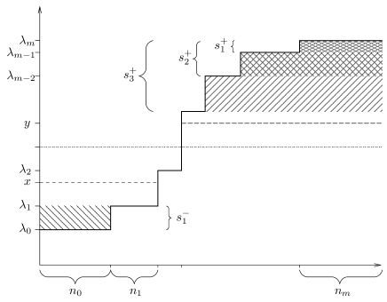
Figure 1: Visualization of the definition of $x$, $y$, and $s_{r}^{\pm}$, together with the eigenvalues $\lambda_{l}$ and multiplicities $n_{l}$ as defined in section IV.2. In this example, we have $b^{-}=1$ and $b^{+}=3$.

In the following, we give an efficient algorithm for calculating the constants $x,y,b^{-}$, and $b^{+}$, which is very similar to the one calculating $S_{0}^{\varepsilon}(\rho_{E})$ in the previous section. Let

$$s_{r}^{+} := \sum\limits_{i=1}^{r}n_{m-i+1}(\lambda_{m-i+1}-\lambda_{m-r}),$$ (28)

$$s_{r}^{-} := \sum\limits_{i=1}^{r}n_{i-1}(\lambda_{r}-\lambda_{i-1}),$$ (29)

for $0\leq r\leq m=n+1$. Then the number of the largest (smallest) different eigenvalues, that can be lowered to $y$ (raised to $x$) is given by

$$b^{\pm}:=\max\{r:s_{r}^{\pm}\leq\varepsilon\}.$$ (30)

With these definitions we find that

$$x = \lambda_{b^{-}}+\frac{\varepsilon-s_{b^{-}}}{\sum_{i=0}^{b^{-}}n_{i}},$$ (31)

$$y = \lambda_{m-b^{+}}-\frac{\varepsilon-s_{b^{+}}}{\sum_{i=0}^{b^{+}}n_{m-i}}.$$ (32)

Having calculated the eigenvalues $\mu_{i}$, the entropy is finally given by

$$S_{2}^{\varepsilon}(\rho_{XE})=-\log_{2}\left(\sum_{i=0}^{b^{-}}n_{i}x^{2}+\sum_{i=b^{-}+1}^{b^{+}-1}n_{i}\lambda_{i}^{2}+\right.\hskip 14.22636pt$$

$$\hskip 142.26378pt\left.\sum_{i=b^{+}}^{m}n_{i}y^{2}\right).$$ (33)

IV.3 Calculation of $H_{0}^{\varepsilon}(\mathbf{X}|\mathbf{Y})$

Recall the definition of the conditional $\varepsilon$-smooth Renyi entropy of order zero,

$$H_{0}^{\varepsilon}(\mathbf{X}|\mathbf{Y}):=\min\limits_{\mathbbm{A}:P(\mathbbm{A})\geq 1-\varepsilon}\left(\max\limits_{\mathbf{y}}\log_{2}|\mathcal{P}_{\mathbbm{A}\mathbf{y}}|\right),$$ (34)

where we have introduced $\mathcal{P}_{\mathbbm{A}\mathbf{y}}:=\{\mathbf{x}:P_{\mathbf{X}\mathbbm{A}|\mathbf{Y}=\mathbf{y}}(\mathbf{x})>0\}$. First note that $H_{0}^{\varepsilon}(\mathbf{X}|\mathbf{Y})$ depends only on the number of elements in the set $\mathcal{P}_{\mathbbm{A}\mathbf{y}}$, i.e. on the number of non-zero entries in the probability distribution $P_{\mathbf{X}\mathbbm{A}|\mathbf{Y}=\mathbf{y}}$. Since in our case all values of $P_{\mathbf{X}|\mathbf{Y}=\mathbf{y}}$ are non-zero for all $\mathbf{y}$ (except for the case of perfect correlations, i.e. $\beta_{0}=1$), the maximization over $\mathbf{y}$ can be omitted. Thus the only restriction on the number of non-zero probabilities comes from $\mathbbm{A}$. The minimization over all these events occurring with probability larger or equal to $1-\varepsilon$ can be tackled in the following way: All relevant events $\mathbbm{A}$ need to be of the form $[\mathbf{X}=\mathbf{x}_{1}]\vee\dots\vee[\mathbf{X}=\mathbf{x}_{k}]$, with $\sum_{i=1}^{k}P_{\mathbf{X}}(\mathbf{x}_{i})\geq 1-\varepsilon$. Since we are looking for the smallest set $\mathcal{P}_{\mathbbm{A}\mathbf{y}}$ ($\mathbf{y}$ being arbitrary), we are interested in those events which are most restrictive, i.e. which have $k$ as small as possible. This means we need to find the smallest number $k$ such that the sum of the $k$ largest probabilities in $P_{\mathbf{X}|\mathbf{Y}=\mathbf{y}}$ is greater or equal to $1-\varepsilon$. To this end we look at the probability distribution (14) and find the following probabilities $p_{l}$ and occurrences $n_{l}$, when we condition on a certain value $\mathbf{y}$:

$$p_{l} := \beta_{0}^{l}\beta_{1}^{n-l}$$ (35)

$$n_{l} := \genfrac{(}{)}{0.0pt}{}{n}{l}(d-1)^{n-l}$$ (36)

In analogy to the calculation of $S_{0}^{\varepsilon}(\rho_{E})$, define

$$s_{r}:=\sum\limits_{i=1}^{r}n_{n-i+1}p_{n-i+1},$$ (37)

with $0\leq r\leq n+1$, to be the sum of the $r$ largest different probabilities $p_{l}$. Then the smallest number $b$ such that the sum of the largest $b$ different probabilities is greater or equal than $1-\varepsilon$ is given by

$$b:=\min\{r:s_{r}\geq 1-\varepsilon\}.$$ (38)

With these definitions we find

$$k=\sum\limits_{i=1}^{b}n_{n-i+1}-\left\lfloor\frac{s_{b}-(1-\varepsilon)}{p_{n-b+1}}\right\rfloor.$$ (39)

Finally, we arrive at

$$H_{0}^{\varepsilon}(\mathbf{X}|\mathbf{Y})=\log_{2}k.$$ (40)

V Results

In the previous section, we calculated the entropies involved in the formula for the achievable key length (8). Each entropy is given as a simple function that can be evaluated numerically in a very efficient way with only $\mathcal{O}(n)$ running time. Note that all results are exact (up to machine precision), since no approximations are needed at all. Still, the parameter $n$ (the number of signals) is crucial in the implementation and we are limited to values of the order $10^{4}$ in this quantity. However, this is not a conceptual limitation: using more powerful computers, it is feasible to push this limit further, but we do not believe that this approach would yield surprising results, in view of the results presented in this section.

Figure 2: Key rate versus signal number $n$ for three different values of the security parameter (from top to bottom: $\varepsilon=0.5,0.2,0.01$) for a fixed error rate in the sifted key $1-\beta_{0}=0.02$. The dashed line is a lower bound of the asymptotic value $\lim_{\varepsilon\rightarrow 0}\lim_{n\rightarrow\infty}\ell/n=0.758059$ found in ren05:sec_proof_pa .

The scenario that we are investigating is described by the following parameters: The number $n$ of (quantum) signals sent from Alice to Bob which are kept during the sifting step, the error rate in the sifted key $1-\beta_{0}$ (see Eq. (10)), the security parameter $\varepsilon$, and the dimensionality $d$ of the quantum systems sent from Alice to Bob. For better accessibility, we plot the secret key rate $r$, which is defined as $r=\ell/n$, rather than the key length $\ell$.

Figure 2 shows a plot of the obtainable key rate $r$, as a function of the number $n$ of signals that were measured in the same basis by Alice and Bob. In this example we keep the error rate fixed at $1-\beta_{0}=0.02$ and show plots for different security parameters $\varepsilon$. The error rate is chosen such that we are looking at the regime where the key rate is large and where a simple pre-processing does not seem to play any role ren05:sec_proof_pa . For comparison, we also plot a lower bound on the secret key which holds for any eavesdropping attack, but is only exact in the limiting case $n\rightarrow\infty$; this result was recently derived by Renner et. al ren05:sec_proof_pa . Our key rates approach the asymptotic value $r=0.758059$ as $n$ grows. From the plot, we recover the result found in ren05:sec_proof_pa that in the limit $n\rightarrow\infty$, the dependence on the security parameter $\varepsilon$ becomes negligible, as the three curves for different $\varepsilon$ approach each other. Note that for a small number of signals the secret key rate shows a considerable deviation from the asymptotic value. For a value of $n=10^{4}$, however, the key rate for even a small $\varepsilon=0.01$ reaches already over 83% of the asymptotic value. To give a comparison with experimental implementations, e.g. the number of signals $n$ (after sifting, but before classical post-processing) in the experiment described in pop04:exp_ent_photons is of the order of $10^{5}$.

A prominent feature of our results are the “oscillations” of the achievable key rate, the amplitude of which decreases as $n$ increases. Analytically, the oscillations arise from the structure of $\ell$ given in Eq. (8), being the difference of the three monotonic functions $S_{2}^{\varepsilon^{\prime}}$, $S_{0}^{\varepsilon^{\prime}}$, and $H_{0}^{\varepsilon^{\prime}}$ where the last two are smoothened versions (see Fig. 3) of a non-continuous function. In the limit $n\rightarrow\infty$, the non-continuities disappear, leading to a monotonic key rate. Up to now, we can give no physical explanation for the non-monotonicity, besides the fact that our formula is just an achievable key rate and thus only a lower bound on the optimal key rate. Moreover, we disregarded the classical pre-processing step in our analysis, and thus the key rate might also increase in some cases. Note that up to now, no one-way pre-processing protocols except for the addition of noise ren05:sec_proof_pa have been studied. It was found that the addition of noise has no effect on the key rate if the correlations between Alice and Bob are almost perfect (as in Fig. 2), but the rate can be increased in the region where $0.88\lesssim\beta_{0}\lesssim 0.92$.

Figure 3: Plot of the three entropies in Eq. (8) constituting the secret key length $\ell$ up to an additive term $2\log_{2}(1/\varepsilon)$. In this example we have $1-\beta_{0}=0.02$ and $\varepsilon=0.5$.

The dependence of the secret key rate on the error rate $1-\beta_{0}$ is visualized in Fig. 4: The secret key rate is only non-negative for error rates smaller than $\approx 0.11$ and gets larger as the error rates $1-\beta_{0}$ is decreased. The key rate for finite $n$ is always smaller than the asymptotic value (unless $1-\beta_{0}=0$), and it increases as $\varepsilon$ increases, i.e. as the required security decreases.

Since our formulas are valid not only for qubits, but also for higher-dimensional systems, we can study the influence of the dimensionality on the obtainable key rate. To be able to compare the efficiency of encoding the information in $d=2,3,4$ dimensions, we introduce the quantity $\tilde{n}:=n^{\prime}d=n(d+1)d$ which quantifies the total resources needed in the protocol: We have already mentioned that the number of signals before ($n^{\prime}$) and after the sifting ($n$) are related by $n=n^{\prime}/(d+1)$, where $d+1$ is the number of different encodings used (we consider the “tomographic protocol”). The factor $d$ accounts for the dimension of the single quantum system. We compute the “effective key rate ” $\ell/\tilde{n}$, i.e. the key length, measured in bits, divided by the “total dimensionality” of the Hilbert space of all signals of the raw key (before the sifting). In this way we have quantified the rate with respect to the number of initial resources needed to create the key. Recall that $1-\beta_{0}=(d-1)\beta_{1}$ is the error rate (in the limit $n\rightarrow\infty$) in the sifted key, which is called quantum bit error rate (QBER) in the case of dimension $d=2$. This quantity gives the fraction of errors per $d$it in the sifted key, which makes it difficult to compare different dimensions, unless one can make reasonable statements about how the error rate $1-\beta_{0}$ scales with $d$, i.e. how the eavesdropper treats different dimensions. Keeping this problem in mind, we see in Fig. 5 the dependence of the effective key rate $\ell/\tilde{n}$ on the error rate $1-\beta_{0}$, for a fixed $\tilde{n}=20000$ and security parameter $\varepsilon=0.1$. We can read off the maximal tolerable error rate for which a secret key can still be extracted and fortify the result found in bru02:optimal_eve , namely that the robustness of a QKD protocol increases as the dimension $d$ of the quantum systems increases. This result also holds if sifting is disregarded, i.e. if we keep $dn$ fixed and look at $\ell/(dn)$. On the other hand, if Alice and Bob are highly correlated ($\beta_{0}\rightarrow 1$), we find the reverse dependence on the dimension: A qubit system yields the highest effective key rate and this rate decreases as the dimension $d$ increases.

Figure 4: Key rate $r$ plotted versus the error rate in the sifted key, $1-\beta_{0}$, for a fixed number of signals $n=20,000$. The three solid lines correspond to different security parameters (from top to bottom: $\varepsilon=0.5,0.2,0.01$). The dashed line is again the asymptotic value $\lim_{\varepsilon\rightarrow 0}\lim_{n\rightarrow\infty}l/n$.

VI Conclusions

We have developed a method for the explicit calculation of the secret key rate in quantum key distribution with a finite number of signals $n$, under the assumption that the eavesdropper only conducts symmetric collective attacks, i.e. the state shared by Alice and Bob after the quantum part of the protocol (cf. section II) has the form $\rho_{AB}^{\otimes n}=[(\beta_{0}-\beta_{1}){{|\phi_{d}^{+}\rangle}{\langle\phi_{d}^{+}|}}+\beta_{1}\mathbbm{1}/d]^{\otimes n}$. At this step, Alice and Bob have to measure this state in the computational basis to obtain the classical bit strings that are the starting point of the classical post-processing. This means that any protocol in which Alice and Bob can ensure that they share such a state and which uses privacy amplification is covered by our analysis. In reality, obtaining knowledge about $\rho_{AB}^{\otimes n}$ is a hard task, but we believe that our analysis of the idealized case helps in solving the challenge of a finite key analysis of a more general scenario.

We have shown that the secret key rate obtainable by our protocol strongly depends on the number of quantum signals sent. Our results suggest that for signal numbers larger than $n\sim 10^{4}$, the asymptotic value for the key rate found by ren05:sec_proof_pa is a good approximation. However, for smaller values of $n$, we find a significantly lower value. This is remarkable

Figure 5: Effective key rate for dimension $d=2$ (solid line), $d=3$ (dashed line), $d=4$ (dotted line), and $d=5$ (chain dotted line) for a fixed $\tilde{n}=20000$ and $\varepsilon=0.1$, plotted versus the error rate in the sifted key $1-\beta_{0}$.

in particular because we restricted our analysis to a symmetric eavesdropping strategy, thereby weakening Eve’s power and potentially increasing the obtainable key rate. In contrast, the result found in ren05:sec_proof_pa covers all eavesdropping attacks and thus the asymptotic value of $r$ is already based on pessimistic assumptions. Therefore, our results suggest that for scenarios with only a few number of signals, significant deviations of the key rate from the asymptotic value are to be expected.

A popular task in the analysis of quantum key distribution is the characterization of the threshold QBER, which is the maximal quantum bit error rate, for which the protocol still yields a non-vanishing key rate. However, even a high threshold QBER does not guarantee a feasible protocol, as the key rate might be arbitrarily close to zero or increase very slowly with decreasing QBER. Our results on the other hand quantitatively characterize the secret key rate with respect to all parameters of the protocol. In particular, we have shown that for $d$-dimensional generalizations of the six-state protocol, larger dimensions give a higher robustness, i.e. more noise is tolerable, but smaller dimensions yield a higher key rate if the the correlations between Alice and Bob are already high.

VII Acknowledgements

We would like to thank Barbara Kraus, Norbert Lütkenhaus, and in particular Renato Renner for valuable discussions. This work was supported by the European Commission (Integrated Project SECOQC).

References

- (1) C. H. Bennett and G. Brassard, in Proceedings of the IEEE International Conference on Computers, Systems, and Signal Processing, Bangalora, India (IEEE, New York, 1985), pp. 175–179.
- (2) C. Bennett, G. Brassard, and N. Mermin, Phys. Rev. Lett. 68, 557 (1992).
- (3) M. Curty, M. Lewenstein, and N. Lütkenhaus, Phys. Rev. Lett. 92, 217903 (2004).
- (4) M. Christandl, R. Renner, and A. Ekert, quant-ph/0402131.
- (5) R. Renner, N. Gisin, and B. Kraus, Phys. Rev. A 72, 012332 (2005).
- (6) U. M. Maurer, IEEE Transactions on Information Theory 39, 733 (1993).
- (7) D. Bruß, Phys. Rev. Lett. 81, 3018 (1998).
- (8) H. Bechmann-Pasquinucci and N. Gisin, Phys. Rev. A 59, 4238 (1998).
- (9) C. Bennett, Phys. Rev. Lett. 68, 3121 (1992).
- (10) A. Ekert, Phys. Rev. Lett. 67, 661 (1991).
- (11) V. Scarani, A. Acín, G. Ribordy, and N. Gisin, Phys. Rev. Lett. 92, 057901 (2004).
- (12) I. Devetak and A. Winter, Phys. Rev. A 68, 042301 (2003).
- (13) R. Renner and R. Koenig, in Second Theory of Cryptography Conference, TCC 2005, Vol. 3378 of LNCS, edited by J. Kilian (Springer, New York, 2005), pp. 407–425, also available at http://arxiv.org/abs/quant-ph/0403133.
- (14) M. Ben-Or et al., in Second Theory of Cryptography Conference, TCC 2005, Vol. 3378 of LNCS, edited by J. Kilian (Springer, New York, 2005), pp. 386–406, also available at http://arxiv.org/abs/quant-ph/0409078.
- (15) R. Renner and S. Wolf, Lecture Notes in Computer Science 3788, 199 (2005).
- (16) A. Rényi, in Proceedings of the 4th Berkeley Symposium on Mathematics, Statistics and Probability (University of California Press, Berkeley, 1960), pp. 547–561.
- (17) D. Bruß et al., Phys. Rev. Lett. 91, 097901 (2003).
- (18) Y. C. Liang et al., Phys. Rev. A 68, 22324 (2003).
- (19) M. Fannes, Commun. Math. Phys. 31, 291 (1972).
- (20) A. Poppe et al., Opt. Express 12, 3865 (2004).
- (21) D. Brußand C. Macchiavello, Phys. Rev. Lett. 88, 127901 (2002).