A semiclassical trace formula for the canonical partition function of one dimensional systems

Abstract

We present a semiclassical trace formula for the canonical partition function of arbitrary one-dimensional systems. The approximation is obtained via the stationary exponent method applied to the phase-space integration of the density operator in the coherent state representation. The formalism is valid in the low temperature limit, presenting accurate results in this regime. As illustrations we consider a quartic Hamiltonian that cannot be split into kinetic and potential parts, and a system with two local minima. Applications to spin systems are also presented.

I Introduction

The quantum partition function ${\cal Z}$ is the basic physical quantity from which all ensemble averages are derived in the canonical formalism salinas ; garrod ; mandl . It is given by the trace of the density operator ${\cal Z}={\rm Tr}\,[\hat{\rho}]$, that can be expressed either as a discrete sum in the microstate energies ${\cal Z}=\sum_{n}e^{-\beta E_{n}}$ or as a continuum integral, ${\cal Z}=1/h\int{\rm d}q\,{\rm d}p\,\rho$, where $\rho$ is some representation of the density operator in phase-space, like the Wigner function wigner or the coherent state average of $\hat{\rho}$. In classical mechanics the density is simply $\rho_{class}=e^{-\beta{\cal H}}$, where ${\cal H}$ is the classical Hamiltonian.

Because of the difficulties in the exact evaluation of ${\cal Z}$, a variety of formal developments have appeared in the literature to include quantum effects in statistical mechanics, without exactly solving the Schrodinger equation. Semiclassical methods, in particular, have attracted a lot o attention feynman ; miller3 ; joras1 ; joras2 ; miller1 ; miller2 . From a more basic point of view, it is well-known that classical statistical mechanics is, in most of cases, unable to reproduce the experimental behavior for $T\rightarrow 0$. A paradigmatic example is the failure at low temperatures of Dulong-Petit law for the specific heat of solids, or more generally, the failure of classical systems in obeying the third law of thermodynamics salinas ; garrod ; mandl . Roughly speaking, this is due to quantum discreteness that becomes relevant in this regime. Given this strong discrepancy between classical and quantum statistical mechanics for $T\rightarrow 0$, it is reasonable to ask what happens in a semiclassical formulation, since it should be somewhere in between the two theories. Therefore, it is desirable to obtain an explicit semiclassical expression for the canonical partition function, from which thermodynamic quantities such as internal energy and entropy can be derived in a closed analytical form in terms of classical ingredients.

A straight, but not particularly effective, procedure in this direction is to replace the exact quantum levels by semiclassical ones in the discrete summation. For 1-D systems, expressions for the energy levels in the WKB approximation are relatively easy to obtain, but the corresponding partition function is inaccurate at low temperatures. More elaborated examples are the Wigner-Kirkwood method, which consists of an expansion of the density matrix in powers of $\hslash\beta=\hslash/k_{B}T$ kirk ; approximate path integral representations feynman ; and phase-space sampling with semiclassical quasi-probability distributions miller3 ; joras1 ; joras2 . All these methods use classical ingredients to represent the density operator, but the procedure presented in miller3 is perhaps the most direct, in the sense that it simply replaces the classical Boltzmann weight by a semiclassical one. In this paper we shall consider a similar method. The procedure is based on the recognition that the evolution operator in quantum mechanics and the Boltzmann operator in statistical physics are formally similar. Explicitly we have the correspondence $e^{-i\hat{{\cal H}}t/\hslash}\rightarrow e^{-\beta\hat{{\cal H}}}$ for $t\rightarrow-i\tau$, with $\tau\equiv\hslash\beta$ (the so-called Wick rotation). The density operator $\hat{\rho}$ is obtained when such a rotation is applied to the diagonal quantum propagator and the partition function is written as a phase-space (or configuration space miller1 ; miller2 ) integral that can be calculated numerically. The ensemble averages are, consequently, also expressed in the form of integrations (see equations (2.16) to (2.18) in miller3 ). This method, in spite of its usefulness in numerical calculations, does not allow for a detailed analysis of the functional dependence of thermodynamic potentials, and other related physical quantities of interest, with the temperature. In this work we show that, in the low temperature limit, the phase space integrals appearing in the semiclassical expressions can actually be performed analytically. The resulting representation of the partition function in terms of classical quantities is similar to a trace formula, involving only equilibrium points and periodic orbits. In order to obtain the semiclassical partition function we shall use the coherent state representation. This choice enables the formalism to be applied in more general situations involving internal degrees of freedom such as spins.

We believe that such a direct semiclassical formula should be of use in theoretical studies and also in numerical applications. Besides, some traditional methods like the Wigner-Kirkwood expansion converge very slowly for small $T$, justifying the particular interest in this region of temperatures. As we shall see, however, the semiclassical calculation of ${\rm Tr}[\hat{\rho}]$ naturally leads to the complicated problem of summing over all periodic orbits of a related classical system. This is a common difficulty in practical applications of semiclassical trace formulas. Fortunatelly, due to the effects of the Wick rotation in the classical equations of motion, we shall see that this problem is not present in some important situations, e. g., one-dimensional potentials with a single minimum.

The paper is organized as follows: in section II we review the concepts of Wick rotation, coherent states and semiclassical propagator. Next we derive the semiclassical formula for the partition function and give explicit expressions for potentials with a single well and multiple wells. In section IV we apply these formulas for three specific systems and compare our results with exact quantum and classical calculations and with other approximations. In section V we outline the extension of the formalism to spin systems. Finally, section VI is devoted to some concluding remarks.

II Preliminary Definitions

The partition function can be written in terms of the quantum density of particles in the coherent state representation as

$${\cal Z}=\int\frac{{\rm d}q\,{\rm d}p}{2\pi\hslash}\,\langle z|\,e^{-\beta\hat{\cal H}}\,|z\rangle=\int\frac{{\rm d}q\,{\rm d}p}{2\pi\hslash}\,\rho(q,p,\beta)\;.$$ (1)

Our procedure to calculate the semiclassical limit of ${\cal Z}$ consists of two main steps: first we perform a Wick rotation in the quantum propagator $\langle z|\,e^{-i\hat{{\cal H}}t/\hslash}\,|z\rangle$. Next we replace the propagator by its semiclassical expression and calculate the integral over $q$ and $p$ explicitly by the saddle point method to obtain ${\cal Z}_{sc}$. In the following subsections we review the basic ingredients of this approach: the Wick rotation, the coherent state representation and the semiclassical propagator. In the next section we calculate ${\cal Z}_{sc}$.

II.1 Wick rotation and classical dynamics

Semiclassical formulas contain classical quantities, such as actions and their derivatives, thus our first step is to understand the effect of the rotation $t\longrightarrow-i\tau$ on these classical ingredients. We start with Newton’s second law. Consider the pair of transformations

$$t=-i\tau\;,\;\;V(q)=-\overline{V}(q)\;,$$ (2)

leading to

$$\frac{{\rm d}^{2}q}{{\rm d}t^{2}}=-\frac{{\rm d}V}{{\rm d}q}\;\longrightarrow\;\ddot{q}=\frac{{\rm d}V}{{\rm d}q}\;\longrightarrow\;\ddot{q}=-\frac{{\rm d}\overline{V}}{{\rm d}q}\;,$$ (3)

where dot means derivative with respect to $\tau$. We see that in order to get back the usual form of the equation after the Wick rotation we have set $V=-\overline{V}$, which means that the classical dynamics with complex time is formally equivalent to real time dynamics with the reversed potential $\overline{V}$ feynman ; miller1 . The effect on the classical action is as follows ($m=1$)

$$S=\int_{0}^{t}{\rm d}t^{\prime}{\cal L}=\int_{0}^{t}{\rm d}t^{\prime}\left[\frac{1}{2}\left(\frac{{\rm d}q}{{\rm d}t}\right)^{2}-V\right]\rightarrow i\int_{0}^{\hslash\beta}{\rm d}\tau^{\prime}\left(\frac{1}{2}\dot{q}^{2}-\overline{V}\right)=i\int_{0}^{\hslash\beta}{\rm d}\tau^{\prime}\,\overline{{\cal L}}=i\,\overline{S}\;,$$ (4)

where it is understood that $\overline{\cal L}$ and $\overline{S}$ in the right-hand side are evaluated for a final time $\hslash\beta$ and with the reversed potential $\overline{V}$. There is, however, a more general approach, that we may call ‘canonical Wick rotation’, which is constructed in phase-space and does not rely on the existence of the function $V(q)$. Starting from Hamilton’s equations and making

$$t=-i\tau\;,\;\;{\cal H}=iH$$ (5)

we obtain

$$\frac{{\rm d}q}{{\rm d}t}=\frac{\partial{\cal H}}{\partial p}\;,\;\;\frac{{\rm d}p}{{\rm d}t}=-\frac{\partial{\cal H}}{\partial q}\;\;\rightarrow\;\;\dot{q}=-i\frac{\partial{\cal H}}{\partial p}\;,\;\;\dot{p}=i\frac{\partial{\cal H}}{\partial q}\;\;\rightarrow\;\;\dot{q}=\frac{\partial H}{\partial p}\;,\;\;\dot{p}=-\frac{\partial H}{\partial q}\;,$$ (6)

which preserve the original form of the canonical equations. If the Hamiltonian can be written in ‘Euclidean’ form ($p^{2}/2+V$) the operations (2) and (5) produce the same overall result. However, for more general Hamiltonians, for example with force fields not derivable from a potential or involving spin degrees of freedom, only the last pair of transformations is applicable. The classical action is invariant under these transformations,

$$S=\int_{0}^{t}{\rm d}t^{\prime}\left[p\left(\frac{{\rm d}q}{{\rm d}t}\right)-{\cal H}\right]\rightarrow\int_{0}^{\hslash\beta}{\rm d}\tau^{\prime}\left(p\dot{q}-H\right)=S\;.$$ (7)

In deriving our semiclassical partition function we shall employ the canonical Wick rotation because of its generality. As illustrations we apply the transformation (5) to a non-Euclidean Hamiltonian and the transformation (2) to a system with a well defined potential in section IV.

II.2 Coherent state representation

Here we briefly describe some properties of the coherent state (or Bargman) representation of quantum mechanics. Canonical coherent states $\{|z\rangle\}$ can be expressed as an infinite sum of harmonic oscillator number states $\{|n\rangle\}$:

$$|z\rangle=e^{-|z|^{2}/2}\sum_{n=0}^{\infty}\frac{z^{n}}{\sqrt{n!}}\,|n\rangle\;,\;\;\mbox{where}\;\;z=\frac{1}{\sqrt{2}}\left(\frac{q}{b}+i\,\frac{bp}{\hbar}\right)\;.$$ (8)

The real numbers $q$ and $p$ are the expectation values of the corresponding quantum operators $\hat{q}$ and $\hat{p}$ in the state $|z\rangle$, while the parameter $b$ is proportional to the uncertainty in position, $b=\sqrt{2}\,\Delta q$, and is related to the frequency of the associated harmonic potential by $b^{2}=\hslash/m\omega$. The resolution of unity can be written in terms of the set $\{|z\rangle\}$ as

$$\hat{I}=\int\frac{{\rm d}\,q{\rm d}p}{2\pi\hslash}\;|z\rangle\langle z|\equiv\int\frac{{\rm d}\,z^{*}{\rm d}z}{2\pi i}\;|z\rangle\langle z|\;.$$ (9)

In the coherent state representation the density of particles in phase-space reads

$$\rho(q,p,\beta)=\langle z|e^{-\beta\hat{{\cal H}}}|z\rangle\;,$$ (10)

whose corresponding quantity under the inverse transformation $\tau=it$ is the diagonal form of the coherent state propagator $K(q,p,t)=\langle z|e^{-i\hat{{\cal H}}t/\hslash}|z\rangle$.

We finish this subsection by defining the canonically conjugated variables $u(t)=[q(t)/b+i\,bp(t)/\hbar]/\sqrt{2}$ and $v(t)=[q(t)/b-i\,bp(t)/\hbar]/\sqrt{2}$ in terms of which Hamilton’s equations read

$$\frac{{\rm d}v}{{\rm d}t}=\frac{i}{\hslash}\frac{\partial{\cal H}}{\partial u}\;,\;\;\frac{{\rm d}u}{{\rm d}t}=-\frac{i}{\hslash}\frac{\partial{\cal H}}{\partial v}\;.$$ (11)

These variables are particularly convenient to write down the semiclassical limit of the coherent state propagator.

II.3 Semiclassical coherent state propagator

The set of coherent states forms a non-orthogonal over-complete basis, since each state in the set can be written as a linear combination of the others. This over-completeness implies the existence of several forms of the path integral formulation for the propagator, all equivalent quantum mechanically, but each leading to a slightly different semiclassical limit. Klauder and Skagerstam Klau85 proposed two basic forms for the coherent state path integral. The semiclassical limit of these propagators were considered in marcus where it was shown that both propagators can be written in terms of classical complex trajectories, each governed by a different classical representation of the Hamiltonian operator $\hat{{\cal H}}$: the P representation in one case and the Q representation in other. The phase appearing in these semiclassical formulas turns is not just the action of the corresponding complex classical trajectory, but it also contains a ‘correction term’ that comes with different signs in each formula. In marcus it was also suggested that a semiclassical representation involving directly the Weyl representation of $\hat{{\cal H}}$, or the classical Hamiltonian ${\cal H}$, could probably be constructed, and a formula for this representation was conjectured. This conjecture, along with the corresponding quantum mechanical path integral representation, has been recently proved coelho using the translation and reflection operators studied in ozorio . In this paper we shall adopt this later semiclassical expression, since it is the simplest (although not always the most accurate Pol03 ) of the three known formulas. This semiclassical expression for the propagator connecting an initial state $|z^{\prime}\rangle$ to a final state $|z^{\prime\prime}\rangle$ is given by

$$\langle z^{\prime\prime}|e^{-\frac{i}{\hslash}\hat{\cal H}t}|z^{\prime}\rangle_{sc}=\sqrt{\frac{1}{M_{vv}}}\;\exp\left\{\frac{i}{\hbar}\Phi(v^{\prime\prime},u^{\prime},t)-\frac{1}{2}(|u^{\prime}|^{2}+|v^{\prime\prime}|^{2})\right\},$$ (12)

where there is an implicit sum over the, usually complex, trajectories satisfying Hamilton’s equations (11) with boundary conditions $u^{\prime}\equiv u(0)=z^{\prime}$, $v^{\prime\prime}\equiv v(t)=z^{\prime\prime*}$. The Hamiltonian entering in formula (12) is the function ${\cal H}$ describing the corresponding classical system, and the function appearing in the exponent is the complex action given by

$$\Phi(v^{\prime\prime},u^{\prime},t)=\int_{0}^{t}\left[\frac{i\hbar}{2}\left(v\frac{{\rm d}u}{{\rm d}t}-u\frac{{\rm d}v}{{\rm d}t}\right)-{\cal H}\right]{\rm d}t^{\prime}-\frac{i\hbar}{2}\left[u^{\prime}v^{\prime}+v^{\prime\prime}u^{\prime\prime}\right]\;,$$ (13)

where we have set $u^{\prime\prime}\equiv u(t)$ and $v^{\prime}\equiv v(0)$. Note that, due to the complex character of the classical orbits, in general, we have $v^{\prime}\neq z^{\prime*}$ and $u^{\prime\prime}\neq z^{\prime\prime}$. Finally, the pre-factor in formula (12) is written in terms of the tangent matrix, whose elements are given by the following relation

$$\begin{pmatrix}\delta u^{\prime\prime}\\ \\ \delta v^{\prime\prime}\end{pmatrix}\equiv\begin{pmatrix}M_{uu}&M_{uv}\\ \\ M_{vu}&M_{vv}\end{pmatrix}\begin{pmatrix}\delta u^{\prime}\\ \\ \delta v^{\prime}\end{pmatrix}\;,$$ (14)

where $(\delta u^{\prime}$, $\delta v^{\prime})$ denote small initial deviations from the classical orbit and $(\delta u^{\prime\prime}$, $\delta v^{\prime\prime})$ the corresponding deviations after a propagation time $t$. It is simple to show that $\det[M]=1$ and that the following relations are valid

$$\frac{i\hslash}{M_{vv}}=-\partial^{2}\Phi/\partial u^{\prime}\partial v^{\prime\prime}\;,\;\;\frac{1}{M_{uv}}=\frac{\partial^{2}\Phi/\partial u^{\prime}\partial v^{\prime\prime}}{\partial^{2}\Phi/\partial{v^{\prime\prime}}^{2}}\;,\;\;\frac{1}{M_{vu}}=-\frac{\partial^{2}\Phi/\partial u^{\prime}\partial v^{\prime\prime}}{\partial^{2}\Phi/\partial{u^{\prime}}^{2}}\;.$$ (15)

III The semiclassical canonical partition function

We proceed to make the transformations $t=-i\tau$ and ${\cal H}=iH$ in Eq.(12) to get the semiclassical density of particles in phase-space. Since the complex action and, consequently, the tangent matrix elements remain invariant, the semiclassical density of particles at a given temperature is

$$\rho_{sc}=\langle z^{\prime}|e^{-\beta\hat{\cal H}}|z^{\prime}\rangle_{sc}=\sqrt{\frac{1}{M_{vv}}}\;\exp\left\{\frac{i}{\hbar}\Phi(v^{\prime\prime},u^{\prime},\tau)-z^{\prime*}z^{\prime}\right\}\;.$$ (16)

We remark that Hamilton’s equations (11) become

$$\dot{v}=\frac{i}{\hslash}\frac{\partial H}{\partial u}\;,\;\;\dot{u}=-\frac{i}{\hslash}\frac{\partial H}{\partial v}\;,$$ (17)

with the boundary conditions (for the diagonal propagator)

$$u(0)=u^{\prime}=z^{\prime}\;,\;\;v(\tau)=v^{\prime\prime}=v(\hslash\beta)=z^{\prime*}\;.$$ (18)

The semiclassical partition function is given by

$${\cal Z}_{sc}=\int\frac{du^{\prime}\,dv^{\prime\prime}}{2\pi i}\sqrt{\frac{1}{M_{vv}}}\;\exp\left\{\frac{i}{\hbar}\Phi(v^{\prime\prime},u^{\prime},\tau)_{v^{\prime\prime}=z^{\prime*},u^{\prime}=z^{\prime}}\;-z^{\prime*}z^{\prime}\right\}\;.$$ (19)

In order to evaluate this integral by stationary exponent approximation we shall assume the low temperature limit $\beta>>1$. The stationarity conditions are

$$\frac{i}{\hslash}\frac{\partial\Phi}{\partial u^{\prime}}-z^{\prime*}=v^{\prime}-z^{\prime*}=0\;,\;\;\frac{i}{\hslash}\frac{\partial\Phi}{\partial v^{\prime\prime}}-z^{\prime}=u^{\prime\prime}-z^{\prime}=0\;$$ (20)

where we used the relations $\partial\Phi/\partial u^{\prime}=-i\hbar v^{\prime}$ and $\partial\Phi/\partial v^{\prime\prime}=-i\hbar u^{\prime\prime}$ marcus . We get

$$v^{\prime}=z^{\prime*}\;,\;\;u^{\prime\prime}=z^{\prime}\;.$$ (21)

Therefore, the trajectories must satisfy the four conditions (18) and (21). It can be shown that these restrictions demand the contributing orbits to be real and periodic. Next we expand the exponent in (19) around the stationary trajectories, labeled with the subscript ‘$0$’, up to second order and evaluate the pre-factor on the contributing solutions. We obtain

$$\begin{array}[]{ll}{\cal Z}_{sc}&=\displaystyle{\left(\frac{e^{\frac{i}{\hslash}\Phi-u^{\prime}v^{\prime\prime}}}{\sqrt{M_{vv}}}\right)_{0}\int\frac{{\rm d}(\Delta u^{\prime})\,{\rm d}(\Delta v^{\prime\prime})}{2\pi i}}\\ \\ &\times\exp{\left\{\frac{i}{2\hslash}\left(\frac{\partial^{2}\Phi}{\partial u^{\prime 2}}\right)_{0}\Delta u^{\prime 2}+\frac{i}{2\hslash}\left(\frac{\partial^{2}\Phi}{\partial v^{\prime\prime 2}}\right)_{0}\Delta v^{\prime\prime 2}+\left(\frac{i}{\hslash}\frac{\partial^{2}\Phi}{\partial u^{\prime}\partial v^{\prime\prime}}-1\right)_{0}\Delta u^{\prime}\Delta v^{\prime\prime}\right\}}\;,\end{array}$$ (22)

where $\Delta u^{\prime}=u^{\prime}-u^{\prime}_{0}$ and $\Delta v^{\prime\prime}=v^{\prime\prime}-v^{\prime\prime}_{0}$. The Gaussian integration gives

$${\cal Z}_{sc}=\left(\frac{e^{\frac{i}{\hslash}\Phi-u^{\prime}v^{\prime\prime}}}{\sqrt{M_{vv}}}\right)_{0}\left[\left(\frac{i}{\hslash}\frac{\partial^{2}\Phi}{\partial u^{\prime}\partial v^{\prime\prime}}-1\right)^{2}+\frac{1}{\hslash^{2}}\frac{\partial^{2}\Phi}{\partial u^{\prime 2}}\frac{\partial^{2}\Phi}{\partial v^{\prime\prime 2}}\right]_{0}^{-1/2}\;.$$ (23)

From relations (15) we obtain the following compact expression for the semiclassical partition function

$${\cal Z}_{sc}=\sum_{j}\frac{e^{\frac{i}{\hslash}\Phi_{0}^{(j)}-{u^{\prime}}^{(j)}_{0}{v^{\prime\prime}}^{(j)}_{0}}}{\sqrt{{\rm Tr}[M^{(j)}_{0}]-2}}\;,$$ (24)

where the sum runs over the real periodic trajectories with period $\hbar\beta$ and Tr$[M]=M_{uu}+M_{vv}$. Note that, since the contributing trajectories are periodic, the second term in the right-hand side of expression (13) is exactly $-i\hslash u^{\prime}v^{\prime\prime}$, so we can write the exponent in equation (24) as

$$\frac{i}{\hslash}\int_{0}^{\tau}\left[\frac{i\hbar}{2}\left(v\dot{u}-u\dot{v}\right)-{\cal H}\right]{\rm d}\tau^{\prime}=\frac{i}{\hslash}\int_{0}^{\tau}(p\dot{q}-{\cal H}){\rm d}\tau^{\prime}-\frac{i}{2\hslash}pq|_{0}^{\tau}=\frac{i}{\hslash}S\;$$ (25)

where we have used the periodicity in the last equality. Finally, we can write the expression for the semiclassical partition function as

$${\cal Z}_{sc}={\rm Tr}[\hat{\rho}_{sc}]=\sum_{j}Z_{sc}^{(j)}=\sum_{j}\frac{e^{\frac{i}{\hslash}S_{0}^{(j)}}}{\sqrt{{\rm Tr}[M^{(j)}_{0}]-2}}\;.$$ (26)

We remark that, as is usual in stationary phase evaluations, there may exist divergent contributions corresponding to spurious stationary orbits. These orbits must not be taken into account in the semiclassical formula since their inclusion through the deformation of the original integration contours in (19) could not be justified by Cauchy’s Integral Theorem. Note that the expected divergence in the infinite temperature limit occurs for $\tau\rightarrow 0$, when $M$ becomes the identity matrix and Tr$[M^{(j)}_{0}]\rightarrow 2$. Finally, we recall that, had we used transformation (2) instead of (5) the above formula would have $-\overline{S}/\hslash$ as the argument of the exponential. This alternative form is used in the next subsections.

III.1 Single Well Potentials

Now let us assume that there is a potential function $V$ which has a single minimum (corresponding to a maximum of $\overline{V}$). Due to the inversion in concavity, there are no periodic trajectories, except for the trivial orbit that, without loss of generality, we place at $u=v=0$ (or $q=p=0$). So, in this important case, the summation in (26) reduces to a single term calculated on the trivial orbit:

$${\cal Z}_{sc}=\frac{e^{-\frac{1}{\hslash}\overline{S}_{0}}}{\sqrt{{\rm Tr}[M_{0}]-2}}\;.$$ (27)

Formula (27) can be evaluated more explicitly. We have the following relations for the time evolution of small perturbations:

$$\delta\dot{q}=\delta p\;,\;\;\delta\dot{p}=-\frac{\partial^{2}\overline{V}}{\partial q^{2}}\delta q\;.$$ (28)

For a non-trivial trajectory the coefficient $\partial^{2}\overline{V}/\partial q^{2}\equiv\overline{V}^{\prime\prime}$ is a time dependent function, since it must be evaluated on the trajectory $q(\tau)$, but for the trivial orbit it is simply a constant calculated at the maximum of $\overline{V}$, and the above equations can be readily integrated. The result is ${\rm Tr}[M_{0}]=2\cos(\sqrt{\overline{V}^{\prime\prime}}\;\tau)=2\cosh(\sqrt{V^{\prime\prime}}\;\tau)$, where $V^{\prime\prime}>0$. This leads to the following semiclassical partition function

$${\cal Z}_{sc}=\frac{e^{-\beta V(0)}}{2\sinh\left(\frac{1}{2}\hslash\sqrt{V^{\prime\prime}}\beta\right)}\;.$$ (29)

The above expression is simply the partition function for the harmonic oscillator that best fits $V$ at $q=0$. This result turns out to be too poor and the conclusion is that a higher order approximation is needed in this case. In section IV we illustrate such a higher order expansion for a specific example. In contrast, we shall show that the second order semiclassical partition function given by (26) already gives non-trivial results in the case of potentials with multiple minima.

III.2 Multiple Well Potentials

Let us assume that the potential $V$ has $N$ minima, located at $q_{\sigma}$, with $\sigma=1,2,\dots,N$, and $N-1$ local maxima. In this case there are non-trivial periodic orbits between two successive maxima of $\overline{V}$. In addition each equilibrium point corresponds to a trivial orbit that, in principle, should contribute to the evaluation of ${\cal Z}_{sc}$. However, the $N-1$ stable equilibrium points of $\overline{V}$ give rise to terms proportional to $1/\sin\left(\frac{\hslash}{2}\sqrt{\overline{V}^{\prime\prime}}\beta\right)$, $\overline{V}^{\prime\prime}>0$, which have an oscillatory and divergent behavior for $\beta\rightarrow\infty$, and correspond to the spurious saddle points we have mentioned. Discarding these contributions we get

$${\cal Z}_{sc}=\sum_{\sigma=1}^{N}\frac{e^{-\beta V(q_{\sigma})}}{2\sinh\left(\frac{1}{2}\hslash\sqrt{V^{\prime\prime}|_{\sigma}}\beta\right)}+{\sum_{\mu}}^{\prime}\frac{e^{-\frac{1}{\hslash}\overline{S}_{0}^{(\mu)}}}{\sqrt{{\rm Tr}[M^{(\mu)}_{0}]-2}}\;,$$ (30)

where we have split the sum in the trivial unstable equilibria (with respect to $\overline{V}$) and the non-trivial periodic orbits (denoted by the primed sum). We call the first term the harmonic contribution and the second term the tunneling contribution, since the $\mu$-orbits connect successive minima in the original potential. The calculation of the tunneling terms requires a careful procedure. For a fixed temperature $T$ we must seek, in each well of $\overline{V}$, orbits with period $\tau=\hslash/k_{B}T$ and sum their contributions. Note also that these orbits should, in principle, contribute to the partition function at temperatures $T/2$, $T/3$,…, $T/n$, corresponding to the propagation times $2\tau$, $3\tau$,…, $n\tau$. However, these multiple traversal period orbits have larger and larger actions for increasing values of $n$, causing their contribution to fall off exponentially.

III.3 Connection with thermodynamics

The connection between the canonical ensemble in statistical mechanics and thermodynamics can be made through relation ${\cal Z}=\exp(-\beta f)$, where $f$ is the Helmholtz free energy per particle, whose semiclassical expression reads $f_{sc}=-k_{B}T\ln({\cal Z}_{sc})$. The internal energy can also be easily expressed in terms of classical quantities. Using the general formula (26) we obtain

$$u_{sc}=-\frac{\partial}{\partial\beta}\ln{\cal Z}_{sc}=\frac{1}{{\cal Z}_{sc}}\sum_{j}Z_{sc}^{(j)}\left\{{\cal H}_{0}^{(j)}+\frac{1}{2}\frac{\partial}{\partial\beta}\ln({\rm Tr}[M_{0}^{(j)}]-2)\right\}\;,$$ (31)

where we have used $\partial S/\partial\tau=-H=i{\cal H}$. Once we get the Helmholtz and internal energies we can determine the semiclassical expression for the entropy through relation $s=(u-f)/T=k_{B}\beta(u-f)$. In the next section we give an example of a system that classically violates the third law, and show that, on the contrary, the semiclassical entropy does satisfy the condition $s\rightarrow 0$ for $T\rightarrow 0$. Higher order derivatives of thermodynamical interest can also be obtained analytically, e. g., the specific heat $\partial u_{sc}/\partial T$:

$$c_{sc}=-k_{B}\beta^{2}u_{sc}^{2}+\frac{k_{B}\beta^{2}}{{\cal Z}_{sc}}\sum_{j}Z_{sc}^{(j)}\left[\left\{{\cal H}_{0}^{(j)}+\frac{1}{2}\frac{\partial}{\partial\beta}\ln({\rm Tr}[M_{0}^{(j)}]-2)\right\}^{2}-\frac{1}{2}\frac{\partial^{2}}{\partial\beta^{2}}\ln({\rm Tr}[M_{0}^{(j)}]-2)\right]\;.$$ (32)

In the next section we shall apply our formalism to simple examples and compare the results with the pure classical and quantum ones.

IV Applications

IV.1 The simple harmonic Hamiltonian

We first illustrate our semiclassical procedure with the simple harmonic oscillator. The Hamiltonian is

$${\cal H}=\frac{1}{2}p^{2}+\frac{1}{2}\omega^{2}q^{2}=\hslash\omega uv\;\Rightarrow\;H=-i\hslash\omega uv\;.$$ (33)

The solutions of the equations of motion (17) are $u(\tau^{\prime})=u^{\prime}\,e^{-\omega\tau^{\prime}}$, $v(\tau^{\prime})=v^{\prime\prime}\,e^{\omega(\tau^{\prime}-\tau)}$, with $u(0)=z^{\prime}$ and $v(\tau)=z^{\prime*}$. From these relations we can write $u^{\prime\prime}=u^{\prime}\,e^{-\omega\tau}$ and $v^{\prime\prime}=v^{\prime}\,e^{\omega\tau}$, or $\delta u^{\prime\prime}=\,e^{-\omega\tau}\delta u^{\prime}$ and $\delta v^{\prime\prime}=\,e^{\omega\tau}\delta v^{\prime}$. Therefore

$$M_{uu}=\,e^{-\omega\tau}\qquad M_{vv}=\,e^{\omega\tau}\;.$$ (34)

The only periodic trajectory is $u=v=0$, for which the complex action vanish. Gathering the ingredients together we get the exact quantum result for the partition function

$${\cal Z}_{sc}=\frac{1}{\sqrt{e^{\hslash\omega\beta}+e^{-\hslash\omega\beta}-2}}=\frac{1}{2\sinh\left(\frac{\hslash\omega\beta}{2}\right)}\;.$$ (35)

This expression leads to the well-known results for an ensemble of non-interacting harmonic oscillators. In particular, we get for $c_{sc}$ the Einstein expression for the specific heat of a crystalline solid ($c_{sc}=c_{einstein}$).

IV.2 The quartic non-Euclidean Hamiltonian: quadratic approximation

We now consider a more challenging system described by the Hamiltonian

$${\cal H}=\frac{1}{\hslash\omega}\left(\frac{1}{2}p^{2}+\frac{1}{2}\omega^{2}q^{2}+\lambda\right)^{2}=\hslash\omega(uv+\alpha)^{2}\;,$$ (36)

with $\alpha=\lambda/\hslash\omega$. With the Wick rotation we get

$$H=-i\hslash\omega(uv+\alpha)^{2}.$$ (37)

Note that this Hamiltonian may be seen as a sum of a harmonic term (proportional to $\alpha$) and an anharmonic quartic term (independent of $\alpha$). Since $\alpha\sim\hslash^{-1}$, while $uv\sim\hslash^{0}$, in the semiclassical limit ($\alpha>>1$) the quartic term must be seen as a perturbation added to the harmonic Hamiltonian. Note also that the ${\cal H}$ can not be written as $p^{2}/2+V(q)$. The equations of motion are

$$\dot{v}=2\omega(uv+\alpha)v\;,\hskip 14.45377pt\mbox{and}\hskip 14.45377pt\dot{u}=-2\omega(uv+\alpha)u\;.$$ (38)

Since $(uv+\alpha)=\sqrt{{\cal H}/\hslash\omega}$ is a constant of the motion, the classical solution satisfying the boundary conditions is

$$u(\tau^{\prime})=u^{\prime}\,e^{-\Omega\tau^{\prime}},\;\;\;v(\tau^{\prime})=v^{\prime\prime}\,e^{\Omega(\tau^{\prime}-\tau)}\;\Rightarrow\;u^{\prime\prime}=u^{\prime}\,e^{-\Omega\tau},\;\;\;v^{\prime\prime}=v^{\prime}\,e^{\Omega\tau}\;,$$ (39)

where $\Omega=2\omega(u^{\prime}v^{\prime}+\alpha)$ and $\tau=\hslash\beta$. We note that the only periodic orbit is the trivial one, although the system does not involve a potential. The above solution is very similar to that of the harmonic Hamiltonian but, in the present case, the frequency $\Omega$ is energy dependent. The connection between initial and final variations in a given trajectory can be obtained from

$$\delta u^{\prime\prime}=\,e^{-\Omega\tau}\delta u^{\prime}-\tau e^{-\Omega\tau}\delta\Omega\;,\;\;\delta v^{\prime\prime}=\,e^{\Omega\tau}\delta v^{\prime}+\tau e^{\Omega\tau}\delta\Omega\;,$$ (40)

where $\delta\Omega=2\omega(u^{\prime}\delta v^{\prime}+v^{\prime}\delta u^{\prime})$. Therefore the relevant tangent matrix elements are

$$M_{uu}=(1-2\omega\tau u^{\prime}v^{\prime})\,e^{-\Omega\tau}\;,$$ (41)

and

$$M_{vv}=(1+2\omega\tau u^{\prime}v^{\prime})\,e^{\Omega\tau}\;.$$ (42)

On the trivial trajectory $u=v=0$ we obtain simply

$$M_{uu}=e^{-2\alpha\hslash\omega\beta},\quad M_{vv}=e^{2\alpha\hslash\omega\beta},\quad\frac{i}{\hslash}S_{0}=-\alpha^{2}\hslash\omega\beta\;,$$ (43)

where we have set $\Omega=2\omega\alpha$. This leads to the semiclassical result

$${\cal Z}_{sc}=\frac{e^{-\alpha^{2}\hslash\omega\beta}}{2\sinh(\alpha\hslash\omega\beta)}\;,$$ (44)

from which one can write

$$f_{sc}=\alpha^{2}\hslash\omega+\frac{1}{\beta}\ln[2\sinh(\alpha\hslash\omega\beta)]\;,$$ (45)

and

$$u_{sc}=\alpha^{2}\hslash\omega+\hslash\omega\alpha\coth(\alpha\hslash\omega\beta)\;.$$ (46)

Not surprisingly, these expressions correspond to the exact quantum result for the harmonic part of the Hamiltonian (36). In the next subsection we develop a more accurate approximation. The exact quantum partition function is given by ${\cal Z}=\sum_{n}e^{-\beta E_{n}}$, where $\{E_{n}\}$ are the (non-degenerate) eigenvalues of the quantum Hamiltonian $\hat{\cal H}=\hslash\omega(\hat{a}^{\dagger}\hat{a}+\alpha)^{2}$. Thus

$${\cal Z}=\sum_{n}e^{-\hslash\omega\beta(n+\alpha+1/2)^{2}}\;.$$ (47)

The classical function is given by

$${\cal Z}_{class}=\int\frac{{\rm d}\,q{\rm d}p}{2\pi\hslash}\,e^{-\beta{\cal H}}=\frac{\sqrt{\pi}}{2\,\sqrt{\hslash\omega\beta}}\left[1-{\rm Erf}\left(\sqrt{\hslash\omega\beta}\,\alpha\right)\right]\;,$$ (48)

where Erf denotes the error function.

IV.3 The quartic non-Euclidean Hamiltonian: higher order approximation

Higher order corrections to the semiclassical partition function can also be obtained from (19). We illustrate the method for the Hamiltonian (36). Let us rewrite integral (19) as

$${\cal Z}_{sc}=\int\frac{du^{\prime}\,dv^{\prime\prime}}{2\pi i}A\;\exp\left\{\frac{i}{\hbar}\Phi(v^{\prime\prime},u^{\prime},\tau)_{v^{\prime\prime}=z^{\prime*},u^{\prime}=z^{\prime}}\;-z^{\prime*}z^{\prime}\right\}\;,$$ (49)

where $A=1/\sqrt{M_{vv}}$. Our procedure now is to expand the argument of the exponential up to fourth order around the saddle points, and the pre-factor up to second order (for more details see appendix B of marcus ). We get

$$A\approx A_{0}+A_{(u)}\Delta u^{\prime}+A_{(v)}\Delta v^{\prime\prime}+\frac{1}{2}A_{(uu)}\Delta{u^{\prime}}^{2}+\frac{1}{2}A_{(vv)}\Delta{v^{\prime\prime}}^{2}+A_{(uv)}\Delta u^{\prime}\Delta{v^{\prime\prime}}\;,$$ (50)

and

$$\begin{array}[]{ll}\frac{i}{\hbar}\Phi-z^{\prime*}z^{\prime}&\approx\frac{i}{\hslash}\Phi_{0}-u^{\prime}_{0}v^{\prime\prime}_{0}+\frac{i}{2\hslash}\Phi_{(uu)}\Delta u^{\prime 2}+\frac{i}{2\hslash}\Phi_{(vv)}\Delta v^{\prime\prime 2}+\left(\frac{i}{\hslash}\Phi_{(uv)}-1\right)\Delta u^{\prime}\Delta v^{\prime\prime}\\ &+\frac{i}{6\hslash}\left[\Phi_{(uuu)}\Delta{u^{\prime}}^{3}+3\,\Phi_{(uuv)}\Delta{u^{\prime}}^{2}\Delta{v^{\prime\prime}}+3\,\Phi_{(uvv)}\Delta{u^{\prime}}\Delta{v^{\prime\prime}}^{2}+\Phi_{(vvv)}\Delta{v^{\prime\prime}}^{3}\right]\\ &+\frac{i}{24\hslash}\left[\Phi_{(uuuu)}\Delta{u^{\prime}}^{4}+4\,\Phi_{(uuuv)}\Delta{u^{\prime}}^{3}\Delta{v^{\prime\prime}}+6\,\Phi_{(uuvv)}\Delta{u^{\prime}}^{2}\Delta{v^{\prime\prime}}^{2}\right.\\ &\left.+4\,\Phi_{(uvvv)}\Delta{u^{\prime}}\Delta{v^{\prime\prime}}^{3}+\Phi_{(vvvv)}\Delta{v^{\prime\prime}}^{4}\right]\;,\end{array}$$

where $A_{(u)}=(\partial A/\partial u^{\prime})_{0}$ and so on. For the Hamiltonian (36) we find that the only non-vanishing terms are the ones proportional to $A_{(uv)}$, $\Phi_{(uv)}$, and $\Phi_{(uuvv)}$ besides the zeroth order terms (see appendix). Therefore the partition function integral reads

$$\begin{array}[]{ll}\tilde{\cal Z}_{sc}&=e^{\frac{i}{\hslash}\Phi_{0}}\int\frac{{\rm d}(\Delta u^{\prime})\,{\rm d}(\Delta v^{\prime\prime})}{2\pi i}\left(A_{0}+A_{(uv)}\Delta u^{\prime}\Delta{v^{\prime\prime}}\right)\;\times\\ &\qquad\qquad\exp{\left\{\left(\frac{i}{\hslash}\Phi_{(uv)}-1\right)\Delta u^{\prime}\Delta v^{\prime\prime}+\frac{i}{4\hslash}\,\Phi_{(uuvv)}\Delta{u^{\prime}}^{2}\Delta{v^{\prime\prime}}^{2}\right\}}\\ \\ &\approx e^{-\omega\alpha^{2}\hslash\beta}\int\frac{{\rm d}(\Delta u^{\prime})\,{\rm d}(\Delta v^{\prime\prime})}{2\pi i}\left(A_{0}+A_{(uv)}\Delta u^{\prime}\Delta{v^{\prime\prime}}\right)\;\times\\ &\qquad\qquad\left(1+\frac{i}{4\hslash}\,\Phi_{(uuvv)}\Delta{u^{\prime}}^{2}\Delta{v^{\prime\prime}}^{2}\right)\,\exp{\left\{\left(\frac{i}{\hslash}\Phi_{(uv)}-1\right)\Delta u^{\prime}\Delta v^{\prime\prime}\right\}}\;,\end{array}$$ (51)

where we have assumed that the fourth order contribution in the exponent is small if compared to the second order term, and the tilde indicates the higher order approximation. The next step is to diagonalize the quadratic form in the argument of the exponential. This can be done with the variables $W$ and $K$ given by

$$\Delta u^{\prime}=\frac{1}{\sqrt{2\,\gamma}}(K-iW)\;,\;\;\Delta v^{\prime\prime}=-\frac{1}{\sqrt{2\,\gamma}}(K+iW)\;,$$ (52)

where $2\,\gamma\equiv(i\Phi_{(uv)}/\hslash-1)$. Integral (51) becomes

$$\tilde{\cal Z}_{sc}=\frac{e^{-\omega\alpha^{2}\hslash\beta}}{i\,\gamma}\int\frac{{\rm d}W\,{\rm d}K}{2\pi i}\left[A_{0}-\frac{A_{(uv)}}{2\gamma}(W^{2}+K^{2})+\frac{iA_{0}\Phi_{(uuvv)}}{16\,\hslash\gamma^{2}}(W^{2}+K^{2})^{2}\right]\,e^{-W^{2}-K^{2}}\;,$$ (53)

where we have excluded terms of order higher than four. The resulting partition function is

$$\tilde{\cal Z}_{sc}={\cal Z}_{sc}\left(1-\frac{A_{(uv)}}{2\gamma A_{0}}-\frac{\Phi_{(uuvv)}}{i8\hslash\gamma^{2}}\right)\;,$$ (54)

where ${\cal Z}_{sc}$ is given by expression (44). We have find that (see appendix)

$$A_{0}=e^{-\alpha\hslash\omega\beta}\;,\;\;A_{(uv)}=-2\hslash\omega\beta\,e^{-3\,\alpha\hslash\omega\beta}\;,\;\;\Phi_{(uuvv)}=4i\,\hslash^{2}\omega\beta\,e^{-4\,\alpha\hslash\omega\beta}\;,$$ (55)

and, therefore,

$$\tilde{\cal Z}_{sc}=\frac{e^{-\alpha^{2}\hslash\omega\beta}}{2\sinh(\alpha\hslash\omega\beta)}\left(1-\frac{\hslash\omega\beta}{2}\left[\sinh(\alpha\hslash\omega\beta)\right]^{-2}\right)\;.$$ (56)

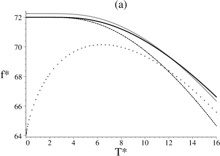
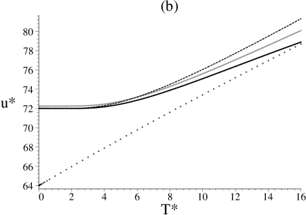
Figure 1: Scaled Helmholtz free energy (a) and scaled internal energy (b): higher order semiclassical (black), quantum (gray), classical (crosses), and quadratic semiclassical (dashed line).

In figure 1 we compare the scaled thermodynamic potentials $f^{*}=f/\hslash\omega$ and $u^{*}=u/\hslash\omega$ as functions of the reduced temperature $T^{*}=k_{B}T/\hslash\omega$, with $\alpha=8.0$, for the four cases: higher order semiclassical (black), quantum (gray), classical (crosses), and quadratic semiclassical (dashed line). As expected the classical results tend to the exact quantum ones for high temperatures, while they completely fail to describe the physical behavior at $T\rightarrow 0$. In contrast, the semiclassical approximations are very precise in the low temperature limit. In particular we note that the semiclassical entropy satisfies the third law of thermodynamics while the classical function does not. This is shown in figure 2, where the scaled entropy $s^{*}=s/k_{B}$ is plotted as a function of $T^{*}$.

IV.4 Two-Well Potential

Here we address a system with a quartic potential function $V=A\,q^{4}-B\,q^{2}+C$, with $A,B>0$. If we denote the height of the local maximum located at $q=0$ by $\Delta E$ and the distance between the two symmetric minima by $2a$, the potential is written as

$$V(q)=\Delta E\left[\left(\frac{q}{a}\right)^{4}-2\left(\frac{q}{a}\right)^{2}+1\right]\;,$$ (57)

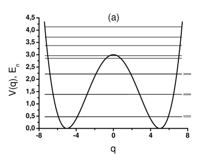
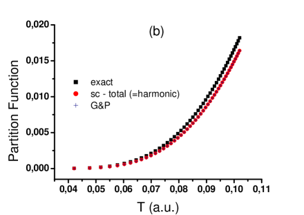
Figure 3: The deep double-well is shown together with the first eleven energy levels in (a). In (b) the exact, semiclassical, and G&P results are compared.

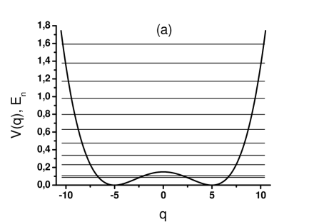
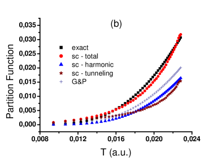
Figure 4: The shallow double-well is shown together with the first eleven energy levels in (a). In (b) the exact, total semiclassical, harmonic contribution, tunneling contribution, and G&P results are displayed.

such that $V(\pm a)=0$. In this case we apply equation (30) directly. The harmonic contribution is $2\times 1/[2\sinh(\hslash\sqrt{2\Delta E}\beta/a)]$, while the tunneling term must be determined numerically. There are two distinct regimes to be considered. If $\Delta E$ is large enough to encompass several energy levels, the harmonic contribution should be dominant over the tunneling one, since the two minima hardly ‘see’ each other. In this case the trajectories connecting the wells have large actions, giving exponentially small contributions to the semiclassical partition function. In contrast, when $\Delta E$ is comparable with the energy of the ground state, the tunneling term should give a relevant contribution. These statements are verified in the numerical computation of ${\cal Z}_{sc}$ for $\Delta E=3.0$ and $\Delta E=0.15$ with $a=5$ in both cases (we use arbitrary units for which $\hslash=1$ and $k_{B}=1$). In the first case (deep well) the ground state has an approximate energy of $0.5$, and there are eight levels (four doublets) with energy smaller than $\Delta E$, as shown in fig. 3(a). Figure 3(b) shows the quantum partition function and ${\cal Z}_{sc}$, where we have used only the harmonic term, since the tunneling contribution is about three orders of magnitude smaller. The approximation derived by Gildener and Patrascioiu GP (see also Har78 ) specifically for the potential (57) is also displayed. This approximation and the semiclassical one produce almost identical results in this case. In the case of the shallow well there are only two levels with energy below $\Delta E=0.15$ (see fig 4(a)). As expected the harmonic contribution is unable to give a good approximation to ${\cal Z}$ and the tunneling term must be considered. The overall semiclassical result is in very good agreement with the exact one, as can be verified from fig 4(b). In this case, the G$\&$P formula does not agree with the quantum result. In the computation of the tunneling term we have not considered multi-period trajectories, since we have found that the corresponding contributions are vanishingly small.

V Spin Systems

As discussed in the beginning of section II.c, the coherent state propagator can be described by a variety of semiclassical expressions. For simplicity we chose the one involving the classical Hamiltonian ${\cal H}$. For spin systems there is no direct classical Hamiltonian and we have to use a different representation. Our starting point is the spin coherent state, defined by $|w\rangle=(1+w^{*}w)^{-s}\exp\{w\hat{S}_{+}/\hslash\}|s,-s\rangle$, where $\hslash s$ is the total spin and $w$ is a complex number. The Q-representation of the Hamiltonian operator is defined as ${\cal H}\equiv\langle w|\hat{\cal H}|w\rangle$. This function appears naturally in the first form of path integral suggested by Klauder and Skagerstan Klau85 , whose semiclassical limit requires the addition of an extra term in (13) marcus , the so-called Solari-Kochetov phase solari ; kochetov :

$${\cal I}_{SK}=\frac{1}{4}\int_{0}^{t}\left[\frac{\partial}{\partial w^{*}}\left(\frac{(1+w^{*}w)^{2}}{2s}\frac{\partial{\cal H}}{\partial w}\right)+\frac{\partial}{\partial w}\left(\frac{(1+w^{*}w)^{2}}{2s}\frac{\partial{\cal H}}{\partial w^{*}}\right)\right]{\rm d}t^{\prime}\;.$$ (58)

Furthermore, since $w$ and $w^{*}$ are not canonically conjugated, it is convenient to define new canoncial variables by marcus2

$$Q=i\sqrt{\frac{s}{1+w^{*}w}}\,(w^{*}-w)\;,\;\;P=\sqrt{\frac{s}{1+w^{*}w}}\,(w^{*}+w)\;.$$ (59)

This transformation is the classical analogue of the Holtein-Primakoff bosonization procedure hp . In these variables, the equations satisfied by the stationary phase trajectories that contribute to the semiclassical propagator are the usual Hamilton’s equation of motion

$$\frac{{\rm d}Q}{{\rm d}t}=\frac{\partial{\cal H}}{\partial P}\;,\;\;\frac{{\rm d}P}{{\rm d}t}=-\frac{\partial{\cal H}}{\partial Q}.$$ (60)

We remark that the Solari-Kochetov term does not change the stationary exponent condition since it already involves second derivatives of the Hamiltonian. With this procedure the formalism we have developed can be readily applied to spin systems. The semiclassical partition function reads

$${\cal Z}_{sc}=\sum_{j}\frac{e^{\frac{i}{\hslash}(S_{0}^{(j)}+{\cal I}_{SK}^{(j)})}}{\sqrt{{\rm Tr}[M^{(j)}_{0}]-2}}\;,\;\;\mbox{or}\;\;{\cal Z}_{sc}=\sum_{j}\frac{e^{-\frac{1}{\hslash}(\overline{S}_{0}^{(j)}+\overline{\cal I}_{SK}^{(j)})}}{\sqrt{{\rm Tr}[M^{(j)}_{0}]-2}}\;,$$ (61)

for transformations (5) and (2), respectively.

As a simple example we consider a spin in a uniform magnetic field. The Hamiltonian operator is $\hat{\cal H}=\omega\hat{S}_{z}$, leading to the exact partition function

$${\cal Z}=e^{\hslash\omega\beta s}\sum_{n=0}^{2s}e^{-\hslash\omega\beta n}=\frac{e^{\hslash\omega\beta(s+1/2)}-e^{-\hslash\omega\beta(s+1/2)}}{e^{\hslash\omega\beta/2}-e^{-\hslash\omega\beta/2}}\;.$$ (62)

From the definition of spin coherent states we obtain

$${\cal H}=-\hslash\omega s\left(\frac{1-w^{*}w}{1-w^{*}w}\right)=\hslash\omega\left(\frac{P^{2}}{2}+\frac{Q^{2}}{2}\right)-\hslash\omega s\;,$$ (63)

from which one sees that the only contributing orbit is the trivial one. This yields $iS/\hslash=\hslash\omega\beta s$ and $i{\cal I}_{SK}/\hslash=\hslash\omega\beta/2$. The corresponding semiclassical partition function is

$${\cal Z}_{sc}=\frac{e^{\hslash\omega\beta(s+1/2)}}{e^{\hslash\omega\beta/2}-e^{-\hslash\omega\beta/2}}\;,$$ (64)

which differs from the exact result by a factor that is exponentially small in the low temperature and large spin limits. At first glance it might be expected that the semiclassical result should be exact, since the effective Hamiltonian is quadratic. However, it is important to note that the classical problem we are dealing with is not completely equivalent to that of a harmonic oscillator. In the present case, the phase-space is compact since ${\cal H}\leq\hslash\omega s$ ( see Eq. (63)). The two problems are strictly equivalent only if $s\rightarrow\infty$, when the semiclassical result is exact.

VI Concluding Remarks

We have obtained a semiclassical trace formula for the canonical partition function in the low temperature limit that does not require sampling and numerical integration in phase-space. The examples presented in sections III and IV show that, in spite of the failure of the classical partition function in describing thermal effects at low temperatures, the appropriate combination of classical ingredients appearing in the semiclassical formula is indeed capable of giving very accurate results in this limit. The quantum corrections come precisely in the way we combine the classical functions. The two and three-dimensional extensions of the formalism are straightforward in the case of single minimum potentials.

In the case of multiple minima, the calculation of the non-trivial periodic orbits is more involved due to the higher dimensionality. However, contrary to the situation in usual trace formulas, only very long orbits should contribute in the low temperature regime. In particular, heteroclinic orbits connecting the top of the inverted wells should be of great importance. Calculations for two-dimensional potentials are currently under way. Other potentially interesting perspectives are also open, such as the inclusion of spin-orbit interactions, whose semiclassical propagator has been recently derived piza .

Appendix A Expansion coefficients

In this appendix we indicate how to obtain the equalities (55). The first expression is immediate

$$A_{0}=\sqrt{\frac{1}{M_{vv}}}=e^{-\omega\alpha\hslash\beta}\;,$$ (65)

where we have used the second relation in (43). Now let us calculate $A_{(u)}$. We have

$$A_{(u)}=\left(\frac{\partial A}{\partial u^{\prime}}\right)_{0}=-\left(\frac{1}{2\,M_{vv}^{3/2}}\frac{\partial M_{vv}}{\partial u^{\prime}}\right)_{0}\;.$$ (66)

From equation (42) we have $M_{vv}=(1+2\omega\tau u^{\prime}v^{\prime})\,e^{\Omega\tau}$, which in terms of the independent variables $u^{\prime}$ and $v^{\prime\prime}$ becomes $M_{vv}=(e^{\Omega\tau}+2\omega\tau u^{\prime}v^{\prime\prime})$. Therefore

$$\frac{\partial M_{vv}}{\partial u^{\prime}}=2\omega\tau v^{\prime\prime}+\tau\frac{\partial\Omega}{\partial u^{\prime}}\,e^{\Omega\tau}\;.$$ (67)

One can implicitly determine the derivative of $\Omega$ starting from $\Omega=2\omega(u^{\prime}v^{\prime}+\alpha)=2\omega(u^{\prime}v^{\prime\prime}\,e^{-\Omega\tau}+\alpha)$. The result is

$$\frac{\partial\Omega}{\partial u^{\prime}}=\frac{2\omega v^{\prime\prime}\,e^{-\Omega\tau}}{1+2\omega\tau u^{\prime}v^{\prime\prime}\,e^{-\Omega\tau}}\;\Rightarrow\;\left(\frac{\partial\Omega}{\partial u^{\prime}}\right)_{0}=0\;.$$ (68)

Consequently we have $\left(\frac{\partial M_{vv}}{\partial u^{\prime}}\right)_{0}=0$ and $A_{(u)}=0$. A similar calculation shows that $A_{(v)}=0$. For $A_{(uv)}$ we get

$$A_{(uv)}=-\frac{1}{2}\left(\frac{1}{M_{vv}^{3/2}}\frac{\partial^{2}M_{vv}}{\partial u^{\prime}\partial v^{\prime\prime}}-\frac{3}{2M_{vv}^{5/2}}\frac{\partial M_{vv}}{\partial u^{\prime}}\frac{\partial M_{vv}}{\partial v^{\prime\prime}}\right)_{0}=-\frac{1}{2}\left(\frac{1}{M_{vv}^{3/2}}\frac{\partial^{2}M_{vv}}{\partial u^{\prime}\partial v^{\prime\prime}}\right)_{0}\;,$$ (69)

with

$$\left(\frac{\partial^{2}M_{vv}}{\partial u^{\prime}\partial v^{\prime\prime}}\right)_{0}=\tau\left(\frac{\partial^{2}\Omega}{\partial u^{\prime}\partial v^{\prime\prime}}\right)_{0}\,e^{2\omega\alpha\tau}+2\omega\tau\;.$$ (70)

From equation (68) we can show that

$$\left(\frac{\partial^{2}\Omega}{\partial u^{\prime}\partial v^{\prime\prime}}\right)_{0}=2\omega\,e^{-2\omega\alpha\tau}\;\Rightarrow\;\left(\frac{\partial^{2}M_{vv}}{\partial u^{\prime}\partial v^{\prime\prime}}\right)_{0}=4\omega\tau\;,$$ (71)

which leads to $A_{(uv)}=-2\omega\tau\,e^{-3\omega\alpha\tau}$. Using the same strategy one can prove that $A_{(uu)}=A_{(vv)}=0$, that all third order derivatives of $\Phi$ vanish at the trivial orbit, and that the only non-vanishing fourth order derivative is

$$\Phi_{(uuvv)}=\left(\frac{i\hslash}{M_{vv}^{2}}\frac{\partial^{2}M_{vv}}{\partial u^{\prime}\partial v^{\prime\prime}}\right)_{0}=4i\hslash\ \omega\tau\,e^{-4\omega\alpha\tau}\;.$$ (72)

Figure 2: Scaled entropy: higher order semiclassical (black), quantum (gray), classical (crosses), and quadratic semiclassical (dashed line). The third law of thermodynamics is satisfied by the semiclassical curves.

References

- (1) S. R. A. Salinas, 2001, Introduction to Statistical Physics (New York: Springer).
- (2) C. Garrod, 1995, Statistical Mechanics and Thermodynamics (New York: Oxford University Press).
- (3) F. Mandl, 1988, Statistical Physics (Chichester: John Wiley).
- (4) M. Hillery, R. F. O‘Connel, M. O. Scully, and E. P. Wigner, Phys. Rep. 106 (1984) 121.
- (5) R. P. Feynman and H. Kleinert, Phys. Rev. A34, 5080 (1986).
- (6) R. M. Stratt and W. H. Miller, J. Chem. Phys. 67, 5894 (1977).
- (7) C. A. A. de Carvalho, R. M. Cavalcanti, E. S. Fraga, and S. E. Joras, Phys. Rev E 61, 6392 (2000).
- (8) C. A. A. de Carvalho, R. M. Cavalcanti, E. S. Fraga, and S. E. Joras, Phys. Rev E 66, 056112 (2002).
- (9) W. H. Miller, J. Chem. Phys. 55, 3146 (1971).
- (10) W. H. Miller, J. Chem. Phys. 58, 1664 (1973).
- (11) J. G. Kirkwood, Phys. Rev. 44, 31 (1933).
- (12) J. R. Klauder and B. S. Skagerstam, 1985, Coherent States, Applications in Physics and Mathematical Physics (Singapore: World Scientific).
- (13) M. Baranger, M.A.M. de Aguiar, F. Keck H.J. Korsch and B. Schellaas, J. Phys. A: Math. Gen. 34, 7227 (2001).
- (14) L.C. dos Santos and M.A.M. de Aguiar, in preparation.
- (15) A. M. Ozorio de Almeida, Phys. Rep. 295, 265 (1998).
- (16) E. Pollak and J. Shao, J. Phys. Chem. A 107, 7112 (2003).
- (17) E. Gildener and A. Patrascioiu, Phys. Rev. D 16, 423 (1977).
- (18) B. J. Harrington, Phys. Rev. D 18, 2982 (1978).
- (19) H. G. Solari, J. Math. Phys. 28, 1097 (1987).
- (20) E. A. Kochetov, J. Math. Phys. 36, 4667 (1995).
- (21) M. A. M. de Aguiar, K.Furuya, C. H. Lewenkopf, and M. C. Nemes, Ann. Phys. 216, 291 (1992).
- (22) T. Holstein and H. Primakoff, Phys. Rev. 58, 1098 (1949).
- (23) A.D. Ribeiro, M.A.M. de Aguiar and A.F.R. de Toledo Piza, J. Phys. A: Math. Gen. 39, 3085 (2006).