Coherent single-photon generation and trapping with practical cavity QED systems

Abstract

We study analytically the dynamics of cavity QED nodes in a practical quantum network. Given a single 3-level $\Lambda$-type atom or quantum dot coupled to a micro-cavity, we derive several necessary and sufficient criteria for the coherent trapping and generation of a single photon pulse with a given waveform to be realizable. We prove that these processes can be performed with practical hardware — such as cavity QED systems which are operating deep in the weak coupling regime — given a set of restrictions on the single-photon pulse envelope. We systematically study the effects of spontaneous emission and spurious cavity decay on the transfer efficiency, including the case where more than one excited state participates in the dynamics. This work should open the way to very efficient optimizations of the operation of quantum networks.

Photons, the elementary constituents of light, are fast and robust carriers of quantum information. Recently, techniques have been found to reversibly produce or trap photons one by one in matter. This inter-conversion capability potentially allows quantum information processing using the best of two worlds: the fast and reliable transport of quantum information via photons, and its storage and processing in matter where interactions between qubits can be made strong. Optical cavities with the ability to concentrate the electro-magnetic field in small regions of space provide a natural interface for photonic and matter qubits. They constitute a key element of quantum networksCirac et al. (1997) in which cavity “nodes” communicate coherently via photonic channelsEnk et al. (1998). The theory of photon absorption and trapping was partially worked out in Yao et al. (2005), extending the initial solution given in Cirac et al. (1997). This approach relies on a carefully designed classical “control” pulse driving a 3-level quantum system in a $\Lambda$ configuration, and numerically shows that (contrary to widely accepted belief) the photon transfer can sometimes be realized in a non-adiabatic (i.e., rapid) way. Until then, both theoryKuhn et al. (1999) and experimentsHennrich et al. (2000); Kuhn et al. (2002); McKeever et al. (2004); Brattke et al. (2001); Keller et al. (2004) aiming at coherent photon emission from a driven cavity-QED system were based on an adiabatic technique called Stimulated Raman Adiabatic Passage (STIRAP), requiring a slowly varying control pulse. Another widely accepted requirement for coherent photon transfer is the one of strong coupling between the cavity and the atomic system. This assumption was also challenged numerically in Ref. Kiraz et al. (2004), where it was shown that (adiabatic) coherent photon generation with high efficiency and indistinguishability was possible in the weak coupling regime. However, there remain a number of open questions regarding this technique: Exactly what kind of single photons can be generated and/or trapped? How fast can their envelopes vary? How far detuned from the cavity resonance can they be, and what Raman detunings can be tolerated in connected cavity nodes? How weak a coupling between cavity and atom can be tolerated, and at what expense in performance? Finally, how sensitive is the transfer technique to characteristics of non-ideal systems with spontaneous emission, spurious cavity decay, or where several excited states contribute to the dynamics?

In this paper, we derive analytical formulas that answer all of these questions, and provide a solid basis for the optimization of quantum networks. When losses are neglected, we show that a single criterion — given by Eq. (1) below — determines the existence condition for a control pulse achieving coherent photon transfer in a 3-level cavity-QED system. This criterion tells us which complex envelope functions $\alpha(t)$ of a single photon pulse are eligible for generation and/or trapping when the characteristics of the cavity-QED system are known. Interestingly, this criterion can be satisfied in the non-adiabatic or in the weak-coupling regime, in the presence of photon-cavity detuning, and for arbitrary Raman detuning $\Delta$ (see Fig. 1), suggesting that quantum networks could be operated even with highly deficient and heterogeneous nodes. When losses are included, we find another criterion for the existence of a control pulse that leaves the node and the waveguide unentangled after transfer, and we provide an analytical expression for the transfer efficiency. We show that very efficient transfer can be realized in the weak coupling regime provided the Purcell factor is sufficiently high, regardless of whether strong coupling is precluded by a low cavity $Q$ (as in solid-state systems) or by a large spontaneous emission rate (as in trapped ions and atoms) when compared to the vacuum Rabi frequency. We generalize the loss analysis to the case where other excited states participate in the dynamics of the transfer.

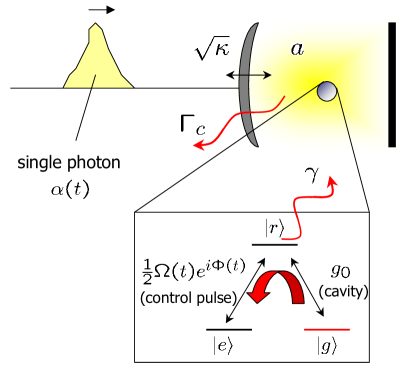
Figure 1: Illustration of a node, a 3-level $\Lambda$ system in a single mode cavity. The red arrow represents the photon trapping process, where a photon from the waveguide is absorbed by the node and induces the flip $\left|{g}\right\rangle\rightarrow\left|{e}\right\rangle$, if the correct control pulse $\Omega(t)$ is applied to the $e-r$ transition. The loss mechanisms are represented by the red wavy arrows.

Consider the system shown in Fig. 1, a 3-level $\Lambda$ atom with ground states $\left|{g}\right\rangle$ and $\left|{e}\right\rangle$ and excited state $\left|{r}\right\rangle$ encapsulated within a single-mode cavity. The cavity vacuum field and coherent control field couple levels $g-r$ and $e-r$ respectively, with Rabi frequency $g_{0}$ and $\frac{1}{2}\Omega(t)$, and common (Raman) detuning $\Delta$. The cavity mode with frequency $\omega_{c}$ leaks into a single waveguide mode, with a rate $\kappa$. The first important result of the paper is the following: in the absence of loss, given an incident single photon pulse with complex amplitude $\alpha(t)e^{-i\omega_{c}t}$ satisfying at all times the criterion

$$\int_{-\infty}^{t}|\alpha(s)|^{2}ds-\frac{|\alpha(t)|^{2}}{\kappa}-\frac{1}{\kappa g_{0}^{2}}|\dot{\alpha}(t)-\frac{\kappa}{2}\alpha(t)|^{2}>0,$$ (1)

there exists a unique control pulse $\Omega(t)=|\Omega(t)|e^{i\Phi(t)}$ that achieves deterministic trapping of the photon, driving the system from initial state $\left|{g}\right\rangle$ to final state $\left|{e}\right\rangle$. Before going into the details of the proof, we study the restrictions imposed by (1). First, note that it is independent of the Raman detuning $\Delta$, so that changing $\Delta$ need not cause any failure as long as the control pulse is changed accordingly. In practice, the intensity and chirp of the control pulse need to increase with $\Delta$, setting experimental limitations on the amount of detuning. Criterion (1) is easier to satisfy if $g_{0}$ is large, and if the photon pulse is slow. In most cases of interest the bandwidth of the photon pulse should be always smaller than both $\kappa$ and $g_{0}^{2}/\kappa$ — bearing in mind that these are estimates that can be violated for short time durations. In the strong coupling regime, this means that the maximum bandwidth of the photon pulse is $\kappa$, irrespective of the cavity coupling. In the weak coupling regime, photon transfer can still occur with efficiencies approaching unity if the photon is slowly varying enough, with a bandwidth not greater than $g_{0}^{2}\kappa$. Finally, we note that the scheme can accommodate a photon-cavity detuning on the order of $g_{0}$; larger detunings would increase the negative contribution of $\dot{\alpha}(t)$ to (1), making the criterion difficult to satisfy in practice.

The second important set of results concern the transfer efficiency in the presence of spontaneous emission from level $\left|{r}\right\rangle$ (with rate $\gamma$) and spurious cavity losses (with rate $\Gamma_{c}$). These dissipative processes are not time-reversal symmetric, so that the photon generation problem has to be handled differently from the photon trapping problem. In both cases, we find a control pulse that achieves the best transfer efficiency possible while leaving the waveguide and the cavity QED node in a separable (unentangled) final state. Technically, such a pulse may not give the absolute highest efficiency for the transfer, but has the key feature that it will minimize the propagation of errors in the network. In the trapping case, the control pulse satisfying the disentanglement condition exists for a certain class of envelope function $\alpha$ obeying a criterion similar to (1), but taking into account the modification of coherent dynamics introduced by $\gamma$ and $\Gamma_{c}$. We will show that the transfer efficiency is given by

$$\eta_{\text{trap}}=\left(1-\frac{\Gamma_{c}}{\kappa}\right)\left(1-\frac{\gamma(\kappa-\Gamma_{c})}{4g_{0}^{2}}\right)-\frac{\gamma}{\kappa g_{0}^{2}}\int|\dot{\alpha}|^{2}$$ (2)

Whether the transfer succeeds or not, the photon has been perfectly removed from the waveguide. In the photon generation case, the eligible photon waveforms are also determined by a modified criterion, and the transfer efficiency is:

$$\eta_{\text{gen}}=\left[\left(1+\frac{\Gamma_{c}}{\kappa}\right)\left(1+\frac{\gamma(\kappa+\Gamma_{c})}{4g_{0}^{2}}\right)+\frac{\gamma}{\kappa g_{0}^{2}}\int|\dot{\alpha}|^{2}\right]^{-1}$$ (3)

These relations indicate that efficient transfer in the presence of losses is possible if the cavity-waveguide interface is well designed ($\Gamma_{c}\ll\kappa$) and if the quantity $4g_{0}^{2}/\kappa\gamma$ (equal to the Purcell factor in the weak coupling regime) is significantly greater than one.

We now prove the above claims and exhibit the corresponding control pulses. We make the simplifying assumptions that there is no additional dephasing of the $e-r$ and $g-r$ transition beyond $\gamma/2$, and we assume that level $\left|{r}\right\rangle$ decays mostly in $\left|{g}\right\rangle$ or outside of the system. Under these conditions it is possible to treat the state of the node as a pure state, defined as

$$\Psi(t)=g(t)\left|{g,1}\right\rangle+r(t)\left|{r,0}\right\rangle+e(t)\left|{e,0}\right\rangle,$$ (4)

where the notation $\left|{X,n}\right\rangle$ stands for the node in level $X$ with $n$ photons in the cavity. Note that $||\Psi(t)||^{2}$ is the probability of finding the excitation in the node (either in the cavity or in the atom) at time $t$. If these conditions do not hold, the state of the system becomes mixed and a density matrix approach is required. In the quantum jump picture Dalibard et al. (1992), the system undergoes a coherent evolution described by $\Psi(t)$, but at each time step it has some probability of collapsing to state $\left|{e,0}\right\rangle$ (due to decay to level $e$) or of undergoing the change $r(t)\rightarrow-r(t)$ (due to dephasing). In this case equations (2) and (3) provide a lower bound for the average fidelity of the transfer.

Using the standard cavity input-output relations Walls and Milburn (1994) and the critical assumption that no more than one photon can be present in the leakage mode of the cavity, we can show that in the rotating wave approximation, the evolution of the waveguide state and of $\Psi(t)$ are given by:

$$\alpha_{out} = \sqrt{\kappa}g-\alpha_{in}$$ (5)

$$\dot{g} = -ig_{0}^{\ast}\,r-\frac{\kappa+\Gamma_{c}}{2}g+\sqrt{\kappa}\alpha_{in}$$ (6)

$$\dot{r} = -(\frac{\gamma}{2}+i\Delta)r-ig_{0}\,g-i\frac{\Omega}{2}\,e$$ (7)

$$\dot{e} = -i\frac{\Omega^{\ast}}{2}\,r$$ (8)

To study the trapping of a photon $\alpha(t)$, we set $\alpha_{in}=\alpha$ and impose the condition $\alpha_{out}=0$. We find that

$$\frac{\Omega}{2}=\frac{i}{e}\left[\dot{r}+\left(\frac{\gamma}{2}+i\Delta\right)r+ig_{0}g\right],$$ (9)

where the necessary and sufficient condition for the existence of $\Omega(t)$ is that $|e|>0$ on all finite time intervals Laudenbach (2000). In the above expression, $g=\alpha/\sqrt{\kappa}$, $r=i(\dot{g}-\frac{\kappa-\Gamma_{c}}{2}g)/g_{0}^{\ast}$, and $e$ is given by

$$|e|^{2} = \left(1-\frac{\Gamma_{c}}{\kappa}\right)\left(1-\frac{\gamma(\kappa-\Gamma_{c})}{4g_{0}^{2}}\right)\int^{t}|\alpha|^{2}-\frac{\gamma}{\kappa g_{0}^{2}}\int^{t}|\dot{\alpha}|^{2}$$ (10)

$$-\frac{|\alpha|^{2}}{\kappa}\left[1-\frac{\gamma(\kappa-\Gamma_{c})}{2g_{0}^{2}}\right]-\frac{|\dot{\alpha}-\frac{(\kappa-\Gamma_{c})}{2}\alpha|^{2}}{\kappa g_{0}^{2}}$$

$$\dot{\Phi}_{e} = \frac{|r|^{2}(\dot{\Phi}_{r}+\Delta)-|g|^{2}\dot{\Phi}_{g}}{|e|^{2}}.$$ (11)

When the right hand side of Eq. (10) is strictly positive at all times, the control pulse exists, and the transfer efficiency is given by $|e|^{2}(t\rightarrow\infty)=\eta_{\text{trap}}$. When trapping occurs, the quantum mechanical amplitude $-\alpha(t)$ associated with the photon being reflected by the front mirror of the cavity exactly cancels the amplitude $\sqrt{\kappa}g(t)$ of the photon being absorbed in the node and re-emitted from it. This destructive interference can be viewed as an impedance-matching requirement between the incoming waveguide and the receiving node that has to be insured by a carefully designed control pulse. Note that for $\Gamma_{c}>\kappa$, we can never find a control pulse that leaves the node and the waveguide unentangled, irrespective of the photon waveform.

In the case of photon generation, we assume that $\alpha_{in}=0$ and we impose $\alpha_{out}=\sqrt{\eta}\,\alpha$, where $\alpha$ is the desired photon envelope normalized to 1, and $\eta$, the generation efficiency, will have to be found self-consistently. The proper control pulse is still given by (9) in this case, but with $g=\sqrt{\eta\alpha/\kappa}$, $r=i(\dot{g}+\frac{\kappa+\Gamma_{c}}{2}g)/g_{0}^{\ast}$, and

$$\frac{1-|e|^{2}}{\eta} = \left(1+\frac{\Gamma_{c}}{\kappa}\right)\left(1+\frac{\gamma(\kappa+\Gamma_{c})}{4g_{0}^{2}}\right)\int^{t}|\alpha|^{2}+\frac{\gamma}{\kappa g_{0}^{2}}\int^{t}|\dot{\alpha}|^{2}$$ (12)

$$+\frac{|\alpha|^{2}}{\kappa}\left[1+\frac{\gamma(\kappa+\Gamma_{c})}{2g_{0}^{2}}\right]+\frac{|\dot{\alpha}+\frac{(\kappa+\Gamma_{c})}{2}\alpha|^{2}}{\kappa g_{0}^{2}}$$

$$\dot{\Phi}_{e} = \frac{|r|^{2}(\dot{\Phi}_{r}+\Delta)-|g|^{2}\dot{\Phi}_{g}}{|e|^{2}}.$$ (13)

The node will be disentangled from the waveguide if and only if $e(t\rightarrow\infty)=0$, that is $\eta=\eta_{\text{gen}}$. The corresponding control pulse then exists if and only if the right hand side of eq. (12) stays strictly positive at all times.

It is worth noting that in the case of zero Raman detuning and when the photon pulse itself has no chirp (i.e. when $\alpha(t)$ can be taken real), then $\Phi(t)$ can be taken constant: no chirp is needed on the control pulse, a potentially desired feature for experiments. If in addition the photon pulse is slow (adiabatic regime) and the cavity coupling is assumed strong, as in many photon generation experiments Hennrich et al. (2000); Kuhn et al. (2002); McKeever et al. (2004); Brattke et al. (2001); Keller et al. (2004), we can obtain a particularly simple relation between control and photon pulse:

$$\left|\frac{\Omega(t)}{2}\right|^{2}\sim\frac{g_{0}^{2}|\alpha(t)|^{2}}{\int_{-\infty}^{t}|\alpha(s)|^{2}\,ds},$$ (14)

with the dual relation

$$|\alpha(t)|^{2}=\frac{\kappa}{g_{0}^{2}}\left|\frac{\Omega(t)}{2}\right|^{2}\,e^{\frac{\kappa}{2g_{0}^{2}}\int_{t}^{+\infty}\,|\frac{\Omega(s)}{2}|^{2}\,ds}.$$ (15)

These expressions explain the experimental observations that a photon emitted with the STIRAP technique will “follow” the control pulse with some retardance due to the finite value of $\kappa$.

We now study the effect of having $N$ excited levels $\left|{r_{k}}\right\rangle$ contributing to the transfer dynamics. We denote as $g_{k}$ and $\Omega_{k}$ respectively the couplings of level $\left|{r_{k}}\right\rangle$ to level $\left|{g}\right\rangle$ and level $\left|{e}\right\rangle$, and we denote as $\Delta_{k}$ and $\gamma_{k}$ the corresponding Raman detuning and spontaneous decay rate from level $r_{k}$. For simplicity, we gather the quantities $r_{k}(t)$, $g_{k}$ and $\Omega_{k}(t)$ into size $N$ vectors $R(t)$, $G$ and $\Omega(t)\,V$, with $V$ a vector of unit length. We also define a complex detuning matrix $\Delta=\text{diag}(\Delta_{k}-i\gamma_{k})$. Using the notation $y\equiv\dot{g}+(\kappa+\Gamma_{c})g/2-\sqrt{\kappa}\alpha_{in}$, the evolution of the system is given by

$$y(t) = -iG^{\dagger}\cdot R(t)$$ (16)

$$\dot{R}(t) = -i\Delta\cdot R(t)-ig(t)\,G-i\frac{\Omega(t)}{2}e(t)V$$ (17)

$$\dot{e}(t) = -i\frac{\Omega^{\ast}(t)}{2}V^{\dagger}\cdot R(t)$$ (18)

The condition for proper trapping is that $y(t)=\dot{g}-(\kappa-\Gamma_{c})g/2$. To find the correct control pulse, we split the vector space into the dimension 1 subspace subtended by vector $V$ and its orthogonal, with corresponding notation $\|$ and $\bot$. With these notations, the above set of equations can be rewritten as :

$$y = -iG_{\|}^{\ast}R_{\|}-iG_{\bot}^{\dagger}\cdot R_{\bot}$$ (19)

$$\dot{R}_{\|} = -i\Delta_{\|}^{\|}R_{\|}-i\Delta_{\bot}^{\|}\cdot R_{\bot}(t)-ig\,G_{\|}-i\frac{\Omega}{2}e$$ (20)

$$\dot{R}_{\bot} = -i\Delta_{\|}^{\bot}R_{\|}-i\Delta_{\bot}^{\bot}\cdot R_{\bot}-ig\,G_{\bot}$$ (21)

$$\dot{e} = -i\frac{\Omega^{\ast}}{2}R_{\|}$$ (22)

When it exists, the correct control pulse envelope function is given by

$$\frac{\Omega}{2}=\frac{i}{e}\left(\dot{R}_{\|}+i\Delta_{\|}^{\|}R_{\|}+i\Delta_{\bot}^{\|}\cdot R_{\bot}+ig\,G_{\|}\right),$$ (23)

where the components of $R$ are given by

$$R_{\|} = \frac{i}{G_{\|}^{\ast}}\left(y+iG_{\bot}^{\dagger}R_{\bot}\right)$$ (24)

$$R_{\bot} = -ie^{-iMt}\int^{t}e^{iMs}\left(G_{\bot}g(s)+i\frac{\Delta_{\|}^{\bot}}{G_{\|}^{\ast}}y(s)\right)$$ (25)

$$M = \Delta_{\bot}^{\bot}-\frac{\Delta_{\|}^{\bot}G_{\bot}^{\dagger}}{G_{\|}^{\ast}}$$ (26)

and the amplitude $e$ is given by

$$|e|^{2} = (1-\frac{\Gamma_{c}}{\kappa})\int^{t}|\alpha|^{2}+2Im(\int^{t}R^{\dagger}\Delta R)$$ (27)

$$-\frac{|\alpha|^{2}}{\kappa}-R^{\dagger}R$$

$$\dot{\Phi}_{e} = \frac{|R_{\|}|^{2}\left[Re(\Delta_{\|}^{\|})+\dot{\Phi}_{R_{\|}}\right]+Re\left[(\Delta_{\bot}^{\|}R_{\bot}+gG_{\|})R_{\|}^{\ast}\right]}{|e|^{2}}$$ (28)

where again the expression for $|e|^{2}$ has to be strictly positive for all times. If $M$ has a purely real eigenvalue, the control pulse must be turned on for an infinite amount of time to prevent re-emission of the photon in the waveguide. Even then, a fraction of the population will be trapped in a “dark” state in the excited states manifold. In general this situation will not happen due to the spontaneous decay. The additional levels will only further reduce the trapping efficiency to a value of

$$\eta_{\text{trap}}^{(N)}=1-\frac{\Gamma_{c}}{\kappa}+2\int R^{\dagger}\,\text{Im}(\Delta)\,R.$$ (29)

The same formula hold for photon generation provided we use $y(t)=\dot{g}+(\kappa+\Gamma_{c})g/2$ and $g=\sqrt{\eta_{\text{gen}}^{(N)}/\kappa}\,\alpha$, with

$$\eta_{\text{gen}}^{(N)}=\left[1+\frac{\Gamma_{c}}{\kappa}+2\int R^{\dagger}\,\text{Im}(\Delta)\,R\right]^{-1}.$$ (30)

Note that the extra absorption caused by the added excited levels increases when $\alpha$ has large Fourier components at frequencies corresponding to the real part of the eigenvalues of $M$. It could be avoided by a clever design the photon envelope.

To summarize, we have derived a series of analytical formulas that clearly delimit the range of operation of cavity QED nodes for quantum networks. With these formulas in hand, we are able to prove that nodes can operate even deeply in the weak coupling regime, at the expense of slowing down the information transfer. Nodes can be operated with an arbitrary atom-cavity detuning $\Delta$ as long as we have the experimental ability to generate a compensating chirp in the control pulses. A significant amount of detuning between cavity photon and cavity resonance can also be tolerated when the vacuum Rabi frequency $g_{0}$ is large. This ability will be key to the operation of heterogeneous cavity QED networks, and suggests that nodes featuring the highest coupling $g_{0}$ will be central to the defect-tolerant operation of the network. For non-ideal systems, we derived an analytical expression of the transfer efficiencies was derived. Spontaneous emission from the excited state causes loss by an amount that is inversely proportional to the Purcell factor (which can be high even in the weak coupling regime). Spurious cavity decay starts to cause prohibitive losses when it becomes comparable to the cavity-waveguide coupling rate. When several excited levels participate in the node dynamics, additional losses occur as some energy becomes irremediably trapped in (and radiated from) a sub-manifold that is not accessible to the control pulse.

The authors acknowledge Charles Santori for his scrupulous examination of the manuscript. This work was supported in part by JST SORST, MURI Grant No. ARMY, DAAD19-03-1-0199 and NTT-BRL.

References

- Cirac et al. (1997) J. Cirac, P. Zoller, H. Kimble, and H. Mabuchi, Phys. Rev. Lett. 78, 3221 (1997).
- Enk et al. (1998) S. V. Enk, J. Cirac, and P. Zoller, Science 279, 205 (1998).
- Yao et al. (2005) W. Yao, R.-B. Liu, and L. Sham, Phys. Rev. Lett. 92, 30504 (2005).
- Kuhn et al. (1999) A. Kuhn, M. Hennrich, T. Bondo, and G. Rempe, Appl. Phys. B 69, 373 (1999).
- Hennrich et al. (2000) M. Hennrich, T. Legero, A. Kuhn, and G. Rempe, Phys. Rev. Lett. 85, 4872 (2000).
- Kuhn et al. (2002) A. Kuhn, M. Hennrich, and G. Rempe, Phys. Rev. Lett. 89, 67901 (2002).
- McKeever et al. (2004) J. McKeever, A. Boca, A. D. Boozer, R. Miller, J. R. Buck, A. Kuzmich, and H. J. Kimble, Science 303, 1992 (2004).
- Brattke et al. (2001) S. Brattke, B. Varcoe, and H. Walther, Science 86, 3534 (2001).
- Keller et al. (2004) M. Keller, B. Lange, K. Hayasaka, W. Lange, and H. Walther, Nature 431, 1075 (2004).
- Kiraz et al. (2004) A. Kiraz, M. Atat re, and A. Imamoglu, Phys. Rev. A 69, 032305 (2004).
- Dalibard et al. (1992) J. Dalibard, Y. Castin, and K. Mølmer, Phys. Rev. Lett. 68, 580 (1992).
- Walls and Milburn (1994) D. Walls and G. Milburn, Quantum Optics (Springer-Verlag, Berlin, 1994).
- Laudenbach (2000) F. Laudenbach, Calcul differentiel et integral (Editions de l’Ecole Polytechnique, 2000).