Effective Hamiltonian approach to adiabatic approximation in open systems

Abstract

The adiabatic approximation in open systems is formulated through the effective Hamiltonian approach. By introducing an ancilla, we embed the open system dynamics into a non-Hermitian quantum dynamics of a composite system, the adiabatic evolution of the open system is then defined as the adiabatic dynamics of the composite system. Validity and invalidity conditions for this approximation are established and discussed. A High-order adiabatic approximation for open systems is introduced. As an example, the adiabatic condition for an open spin-$\frac{1}{2}$ particle in time-dependent magnetic fields is analyzed.

I introduction

As one of the oldest theorems in quantum mechanics, the adiabatic theoremborn28 tells us that if a state is an instantaneous eigenstate of a sufficiently slowly varying Hamiltonian $H(t)$ at one time, then it will remain close to that eigenstate up to a phase factor at later times, while its eigenvalue evolves continuously. The adiabatic theorem underlies the adiabatic approximation scheme, and has potential applications in several areas of physics such as the Landau-Zener transition in molecular physicslandau32 , quantum field theorygell-mann51 and geometric phaseberry84 . Recently, there has been a growing interest in the adiabatic approximation in the context of quantum information, for example, geometric quantum computationzanardi99 ; pachos00 ; jones00 ; duan01 and the new quantum algorithmsfarhi00 ; farhi01 based on the adiabatic approximation.

The concept of adiabaticity has been put forward sarandy05 and applied to quantum informationsarandy105 by Sarandy and Lidar in open systems. In their approach, the open system is described by a master equation $i\dot{\rho}(t)={\cal L}(t)\rho(t)$ $=[H(t),\rho(t)]+L(t)\rho(t)$, and the adiabatic approximation is characterized by independently evolving Jordan blocks, into which the dynamical superoperator ${\cal L}(t)$ can be decomposed. This extension for the adiabaticity in open systems is in a systematic manner, though it is challenging to calculate the superoperator and determine the Jordan decomposition in practice, especially for complicated disturbances $L(t)\rho(t)$. The other extension for the adiabaticity has been presented by Thunström, Åberg and Sjöqvist for weakly open systemsthunstrom05 . In this approach, the eigenspace of the system Hamiltonian are primary instead of instantaneous Jordan blocks. Thus the adiabatic approximation is irrespective of the form of $L(t)\rho(t)$. The main difference between the two approaches is that Sarandy et al. focus on the eigenspace of the entire superoperator ${\cal L}(t)$, while Thunström et al. emphasize the decoupling among the eigenspaces of the system Hamiltonian $H(t)$.

In this paper, we present a new approach to the adiabatic approximation in open systems by introducing an ancilla to couple to the quantum system. An effective Hamiltonian which governs the dynamics of the composite system (quantum system plus ancilla) is derived from the master equation. We then define the adiabatic limit of the open system as the regime in which the composite system evolves adiabatically. The validity and invalidity conditions for this approximation are also given and discussed. An extension to high-order adiabatic approximation is presented. As an example, the adiabatic evolution of a dissipative spin-$\frac{1}{2}$ particle driven by time-dependent magnetic fields is analyzed.

The structure of this paper is organized as follows. In Sec. II we embed the open system dynamics into a non-Hermitian quantum dynamics by introducing an ancilla. The adiabatic approximation is defined, and the validity condition is given in Sec. III. In Sec. IV, we present an example to get more insight on the adiabatic evolution in open systems and discuss the validity condition. Finally we present our conclusions in Sec.V.

II Effective Hamiltonian description for open systems

We begin with the master equation for the density matrix $\rho(t)$gardiner00 ,

$$i\frac{\partial}{\partial t}\rho(t) = [H(t),\rho(t)]-\frac{i}{2}\sum_{k}\{L_{k}^{\dagger}(t)L_{k}(t)\rho(t)$$ (1)

$$+ \rho(t)L_{k}^{\dagger}(t)L_{k}(t)-2L_{k}(t)\rho(t)L_{k}^{\dagger}(t)\}$$

$$= [H(t),\rho(t)]+L(t)\rho(t)$$

$$\equiv {\cal L}(t)\rho(t),$$

where $H(t)$ is a Hermitian Hamiltonian and $L(t)\rho(t)$ describes system-environment couplings and the resulting irreversibility of decoherence, $L_{k}(t)$ may be time-dependent operators describing the system-environment interaction. This master equation is of the Lindblad form, and thus it guarantees the conservation of $\mbox{Tr}\rho(t)$ and the positivity of probabilities. Our aim in this Section is to solve Eq.(1) by introducing an ancilla coupling to the system. This approach was first proposed inyi01 and called effective Hamiltonian approach. The idea of this approach is as the following. The density matrix $\rho(t)$ of the open system can be mapped onto a pure state by introducing an ancilla. The dynamics of the open system is then described by a Schrödinger-like equation with an effective Hamiltonian that can be derived from the master equation. In this way the solution of the master equation can be obtained in terms of the evolution of the composite system by converting the pure state back to the density matrix. To proceed, we assume that the dimension of the system Hamiltonian $H(t)$ is independent of time $t$, so that we may write $H(t)=\sum_{n}^{N}E_{n}(t)|E_{n}(t)\rangle\langle E_{n}(t)|,$ where $N$ is a constant representing the dimension of the system. The ancilla labelled by $A$ is introduced as same as the open system in the sense that its Hilbert space spanned by $\{|e_{m}(0)\rangle\}$ has dimension $N$ and remains unchanged in the dynamics. Thus $\{|E_{n}(0)\rangle\otimes|e_{m}(0)\rangle\}$ may be taken as an orthonormal and complete basis for the composite system. A pure state for the composite system in the $N^{2}$-dimension Hilbert space may be constructed as

$$|\Psi_{\rho}\rangle=\sum_{m,n=1}^{N}\rho_{mn}(t)|E_{m}(0)\rangle|e_{n}(0)\rangle,$$ (2)

where $\rho_{mn}(t)$ are density matrix elements of the open system in the basis $\{|E_{m}(0)\rangle\}$, i.e., $\rho_{mn}(t)=\langle E_{m}(0)|\rho(t)|E_{n}(0)\rangle.$ Clearly, $\langle\Psi_{\rho}(t)|\Psi_{\rho}(t)\rangle={\mbox{T}r}(\rho^{2}(t))\leq 1$, so this pure bipartite state is generally not normalized except that the initial state of the open system is pure and the evolution is unitary. With these definitions, we now try to find an effective Hamiltonian ${\cal H}_{T}(t)$, such that the bipartite pure state $|\Psi_{\rho}(t)\rangle$ satisfies the following Schrödinger-like equation

$$i\frac{\partial}{\partial t}|\Psi_{\rho}(t)\rangle={\cal H}_{T}(t)|\Psi_{\rho}(t)\rangle.$$ (3)

To simplify the derivation, we write the master equation Eq.(1) as

$$i\frac{\partial}{\partial t}\rho(t)={\cal H}(t)\rho(t)-\rho(t){\cal H}^{\dagger}(t)+i\sum_{k}L_{k}(t)\rho(t)L_{k}^{\dagger}(t),$$ (4)

with ${\cal H}(t)=H(t)-i/2\sum_{k}L_{k}^{\dagger}(t)L_{k}(t).$ Substituting equation Eq.(2) together with Eq.(4) into Eq.(3), one finds,

$$i\frac{\partial}{\partial t}|\Psi_{\rho}(t)\rangle = \sum_{m,n,p}\langle E_{m}(0)|{\cal H}(t)|E_{p}(0)\rangle\langle E_{p}(0)|\rho(t)|E_{n}(0)\rangle|E_{m}(0)\rangle|e_{n}(0)\rangle$$ (5)

$$- \langle E_{m}(0)|\rho(t)|E_{p}(0)\rangle\langle E_{p}(0)|{\cal H}^{\dagger}(t)|E_{n}(0)\rangle|E_{m}(0)\rangle|e_{n}(0)\rangle$$

$$+ i\sum_{k}\sum_{m,n,p,q}\langle E_{m}(0)|L_{k}(t)|E_{p}(0)\rangle\langle E_{p}(0)|\rho(t)|E_{q}(0)\rangle\langle E_{q}(0)|L_{k}^{\dagger}(t)|E_{n}(0)\rangle|E_{m}(0)\rangle|e_{n}(0)\rangle$$

$$= \sum_{n}\left[{\cal H}(t)\rho(t)|E_{n}(0)\rangle|e_{n}(0)\rangle-{\cal H}^{A}(t)\rho(t)|E_{n}(0)\rangle|e_{n}(0)\rangle\right]+i\sum_{k,n}L_{k}^{A}(t)L_{k}(t)\rho(t)|E_{n}(0)\rangle|e_{n}(0)\rangle$$

$$\equiv {\cal H}_{T}(t)|\Psi_{\rho}(t)\rangle,$$

where ${\cal H}_{T}(t)$ is defined by

$${\cal H}_{T}(t)={\cal H}(t)-{\cal H}^{A}(t)+i\sum_{k}L_{k}^{A}(t)L_{k}(t),$$ (6)

and referred as the effective Hamiltonian. Operators ${\cal H}(t)$ and $L_{k}(t)$ are for the open system, which take the same form as in Eq.(4), while ${\cal H}^{A}(t)$ and $L_{k}^{A}(t)$ are operators for the ancilla and defined by

$$\langle e_{m}(0)|\hat{O}^{A}|e_{n}(0)\rangle=\langle E_{n}(0)|\hat{O}^{\dagger}|E_{m}(0)\rangle,$$ (7)

with $\hat{O}={\cal H}(t),$ or $L_{k}(t).$ The first two terms in the effective Hamiltonian ${\cal H}_{T}(t)$ describe the free evolution of the open system and the ancilla, respectively, while the third term characterizes couplings between the system and the ancilla. The other works aiming at setting the passage from pure to mixed states in an unitary evolution scheme can be found in Ref.shadwick01 ; reznick96 ; rau02 , but they proceed differently. In Ref.shadwick01 the authors have applied the technique of operator splitting to deal with weakly dissipative systems. The unitary integrator for the Hamiltonian evolution and the conventional integrator for the dissipation were combined to evolve the open system. Based on the wave operator $\hat{\rho}$ defined by the density matrix $\rho$, $\rho=\hat{\rho}\hat{\rho}^{\dagger}$, the unconventional quantum mechanical formalism was proposed in Ref.reznick96 to study the dynamics of open systems. This scheme allows a generalized unitary evolution between pure and mixed states, and sheds new light on the connection between symmetries and conservations laws. Another workrau02 deals with open systems by embedding elements of the density matrix in a higher-dimensional Liouville-Bloch equation. The dissipation and dephasing in the open system were included in the non-Hermitian superoperator. Compared with these schemes, our effective Hamiltonian approach has the advantage that it is easy to calculate, and as will be shown in the next section, the extension for adiabaticity from closed systems to open systems is straightforward.

III The adiabatic approximation in open systems

In this section, we introduce an adiabatic approximation for open systems. Conditions for this approximation are also derived and discussed. We will restrict our discussions to systems where the effective Hamiltonian ${\cal H}_{T}(t)$ is diagonalizable with nondegenerate eigenvalues. For further details we refer the reader to Ref.sokolov06 , where a general discussion on non-Hermitian quantum mechanics is presented.

Let us first define the right and left instantaneous eigenstates of ${\cal H}_{T}(t)$ by

$${\cal H}_{T}(t)|R_{m}(t)\rangle=\lambda_{m}(t)|R_{m}(t)\rangle,$$

$$\langle L_{m}(t)|{\cal H}_{T}(t)=\langle L_{m}(t)|\lambda_{m}(t).$$ (8)

It is easy to show from Eq.(8) that $\langle L_{m}(t)|R_{n}(t)\rangle=\delta_{mn}$ for $\lambda_{m}\neq\lambda_{n}$. Now we are ready to define the adiabatic evolution for open systems, which is directly follow-up from that for closed systems. An open system govern by the master equation Eq.(1) is said to undergo adiabatic evolution if the composite system govern by the effective Hamiltonian ${\cal H}_{T}(t)$ evolves adiabatically. In other words, if the effective Hamiltonian is changed sufficiently slowly, then the composite system in a given non-degenerate eigenstate of the initial effective Hamiltonian ${\cal H}_{T}(0)$ evolves into the corresponding eigenstate of the instantaneous Hamiltonian ${\cal H}_{T}(t)$, without making any population transitions. This leads to the definition of adiabatic evolution in the open system which is the corresponding adiabatic dynamics in the composite system. This definition is a straightforward extension of the idea of adiabatic evolution for open systems, and it will be shown below that the condition for this to occur backs to the conventional adiabatic evolution when the system is a closed system. Let us now derive the validity conditions for open system adiabatic evolution. To this end, we expand $|\Psi_{\rho}(t)\rangle$ for an time $t$ in the instantaneous right eigenstates of ${\cal H}_{T}(t)$ as

$$|\Psi_{\rho}(t)\rangle=\sum_{m}c_{m}(t)e^{-i\int_{0}^{t}\lambda_{m}(\tau)d\tau}|R_{m}(t)\rangle.$$ (9)

Substituting $|\Psi_{\rho}(t)\rangle$ in into the Schrödinger-like equation Eq.(3), one obtains

$$\dot{c}_{m}(t)+\langle L_{m}(t)|\dot{R}_{m}(t)\rangle c_{m}(t)=c_{off}(t),$$ (10)

where

$$c_{off}(t)=-\sum_{n\neq m}c_{n}(t)\langle L_{m}(t)|\dot{R}_{n}(t)\rangle e^{-i\int_{0}^{t}(\lambda_{n}(\tau)-\lambda_{m}(\tau))d\tau}.$$ (11)

Formal integration of Eq.(10) yields,

$$c_{m}(t) = c_{m}(0)-\int_{0}^{t}\langle L_{m}(\tau)|\dot{R}_{m}(\tau)\rangle c_{m}(\tau)d\tau$$ (12)

$$+ \int_{0}^{t}c_{off}(\tau)d\tau.$$

In accordance with the definition of adiabaticity in open systems, the adiabatic regime is obtained when $C_{off}(t)=\int_{0}^{t}c_{off}(\tau)d\tau$ is negligible. This condition ensures that the mixing of coefficients $c_{m}(t)$ corresponding to distinct eigenvalues $\lambda_{m}(t)$ is absent, which in turn guarantees that the change in ${\cal H}_{T}(t)$ is sufficient slow. The latter claim can be shown by rewriting the adiabatic condition $C_{off}(t)\rightarrow 0$ as

$$\Gamma_{mn}(t) = \left|\frac{\langle L_{n}(t)|\partial{\cal H}_{T}(t)/\partial t|R_{m}(t)\rangle}{(\lambda_{m}(t)-\lambda_{n}(t))^{2}}\right|$$ (13)

$$= \left|\frac{\langle L_{n}(t)|\dot{R}_{m}(t)\rangle}{\lambda_{m}(t)-\lambda_{n}(t)}\right|\ll 1.$$

In terms of the density matrix $\rho(t)$, $\langle L_{n}(t)|\dot{R}_{m}(t)\rangle$ can be expressed as $\langle L_{n}(t)|\dot{R}_{m}(t)\rangle={\mbox{T}r}(\rho_{n}(t)\dot{\rho}_{m}(t)),$ where the elements of $\rho_{m}(t)$ are defined as $[\rho_{m}(t)]_{\alpha\beta}=$ $\langle e_{\beta}(0)|\langle E_{\alpha}(0)|R_{m}(t)\rangle$, i.e., $\rho_{m}(t)$ is the density matrix corresponding to the $m$-th right eigenstate of the effective Hamiltonian. Then the adiabatic condition in this case becomes $|{\mbox{T}r}(\rho_{n}(t)\dot{\rho}_{m}(t))|\ll|\lambda_{m}(t)-\lambda_{n}(t)|.$ This relation implies that the transition rate from one path $\rho_{n}(t)$ to the other path $\rho_{m}(t)$ is negligible in the adiabatic evolution.

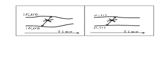
Figure 1: In closed systems, the transition rate among distinct instantaneous eigenstates $\{|E_{m}(t)\rangle\}$of a varying Hamiltonian is zero in adiabatic evolution(left), whereas it is zero among distinct density matrices $\{\rho_{m}(t)\}$ in open systems (right). The distinct density matrices $\rho_{m}(t)$ can be obtained by mapping the instantaneous eigenstates of the effective Hamiltonian back to the open system.

From the other aspect, the adiabatic evolution for open systems indicates that $|\langle L_{m}(t)|\Psi_{\rho}(t)\rangle|$ remains constant in the dynamics for any $m$(degenerate levels are excluded). This results in ${\mbox{T}r}(\rho_{m}(t)\rho(t))=$ constant, showing again that transition rate among distinct paths $\rho_{m}(t)$ is zero in the adiabatic dynamics. A comparison of the adiabatic evolution in closed systems with that in open systems was sketched in figure 1. For a closed system, $L(t)\rho(t)=0$, yielding ${\cal H}_{T}(t)=H(t)-H^{A}(t)$, where $H(t)$ is the system Hamiltonian given in Eq.(1), $H^{A}(t)$ is the counterpart of $H(t)$ for the ancilla. Note that $H^{A}(t)$ takes the same form as $H(t)$, except that it operates on the ancilla. Then the adiabatic condition in this case backs to

$$\left|\frac{\langle E_{m}(t)|\dot{E}_{n}(t)\rangle}{E_{m}(t)-E_{n}(t)}\right|\ll 1.$$ (14)

This is the well known adiabatic condition for closed systemmarzlin04 . In other words, the adiabatic condition defined here for open systems back to the adiabatic condition for closed systems when $L(t)\rho(t)=0,$ showing the consistency of the definition for open systems.

The definition of adiabatic evolution can be easily generalized to high-order adiabatic approximation. To this end, we take the instantaneous eigenspace of the system Hamiltonian $H(t)$ as the primary Hilbert space. As will be shown, this choice has the advantage that the formalism would return straightforwardly to Thunström’s results for weakly open systems. Defining

$$U(t)=\sum_{n}^{N}|E_{n}(0)\rangle\langle E_{n}(t)|,$$ (15)

and

$$\tilde{\rho}(t)=U(t)\rho(t)U^{\dagger}(t),$$ (16)

one gets a master equation for $\tilde{\rho}(t)$ from Eq.(1)thunstrom05 ,

$$i\frac{\partial}{\partial t}\tilde{\rho}(t) = [\tilde{H}(t),\tilde{\rho}(t)]+[Z(t),\tilde{\rho}(t)]$$ (17)

$$- \frac{i}{2}\sum_{k}\{\tilde{L}_{k}^{\dagger}(t)\tilde{L}_{k}(t)\tilde{\rho}(t)+\tilde{\rho}(t)\tilde{L}_{k}^{\dagger}(t)\tilde{L}_{k}(t)$$

$$- 2\tilde{L}_{k}(t)\tilde{\rho}(t)\tilde{L}_{k}^{\dagger}(t)\},$$

where

$$\tilde{H}(t)=\sum_{n}E_{n}(t)|E_{n}(0)\rangle\langle E_{n}(0)|,$$

$$Z(t)=i\dot{U}(t)U^{\dagger}(t),\ \ \tilde{L}_{k}(t)=U(t)L_{k}(t)U^{\dagger}(t).$$

The effective Hamiltonian corresponding to this master equation can be derived by the same procedure and given by

$$\tilde{{\cal H}}_{T}(t)=\tilde{{\cal H}}(t)-\tilde{{\cal H}}^{A}(t)+i\sum_{k}\tilde{L}_{k}^{A}(t)\tilde{L}_{k}(t),$$ (18)

where $\tilde{{\cal H}}(t)=\tilde{H}(t)+Z(t)-\frac{i}{2}\sum_{k}\tilde{L}_{k}^{\dagger}(t)\tilde{L}_{k}(t).$ The high-order adiabatic evolution is then defined as the adiabatic evolution of the composite system with the effective Hamiltonian $\tilde{{\cal H}}_{T}(t)$. The reason of referring the adiabatic approximation with $\tilde{{\cal H}}_{T}(t)$ as the hight-order adiabatic approximation is that $Z(t)$ contains off-diagonal terms $\sum_{m,n}|E_{m}(0)\rangle\langle E_{m}(t)|\dot{E}_{n}(t)\rangle\langle E_{n}(0)|$, $m\neq n$. In the adiabatic approximation defined with ${\cal H}_{T}(t),$ these terms have been ignored when the open system approaches to a closed system. However, they could not be ignored in the latter definition. In fact, the adiabatic approximation defined with $\tilde{{\cal H}}_{T}(t)$ is for $\tilde{\rho}(t)$ in the master equation (17), which is different from $\rho(t)$ in Eq.(1), and this definition is of consistency with the high-order approximation in closed systems. This point can be found by the same analysis presented above for the definition with ${\cal H}_{T}(t)$.

IV example: the adiabatic evolution of an open spin-$\frac{1}{2}$ particle in time-dependent magnetic fields

In this section, we present an example to get more insight of the adiabatic evolution in open systems. The example consists of a dissipative spin-$\frac{1}{2}$ particle driven by a time-dependent magnetic field. The master equation govern the dynamics of such a system can be written as

$$\dot{\rho}=-i[H(t),\rho]+\frac{\kappa}{2}\{2\sigma_{-}\rho\sigma_{+}-\rho\sigma_{+}\sigma_{-}-\sigma_{+}\sigma_{-}\rho\},$$ (19)

where $H(t)=\mu\vec{B}(t)\cdot\vec{\sigma}$ denotes the system Hamiltonian, $\kappa$ stands for the spontaneous emission rate. $\sigma_{i},i=z,+,-$ are Pauli matrices, and $\sigma_{z}=|e\rangle\langle e|-|g\rangle\langle g|$ ($|e\rangle$, denotes the state of spin-up, and $|g\rangle$ spin-down). Suppose $\vec{B}(t)=B_{0}(\sin\theta\cos\phi,\sin\theta\sin\phi,\cos\theta),$ the effective Hamiltonian corresponding to $\rho(t)$ reads,

$${\cal H}_{T}(t)={\cal H}(t)-{\cal H}^{A}(t)+i\kappa\sigma_{-}\tau_{-},$$ (20)

where ${\cal H}(t)=H(t)-\frac{i}{2}|e\rangle\langle e|,$ ${\cal H}^{A}(t)=H^{A}(t)+\frac{i}{2}|e\rangle_{A}\langle e|,$ and $\tau_{-}=|g\rangle_{A}\langle e|$ represents the Pauli matrix of the ancilla. In a subspace spanned by $\{|gg\rangle,|ge\rangle,|eg\rangle,|ee\rangle\}$, the effective Hamiltonian can be written as (in units of $\mu B_{0}$),

$${\cal H}_{T}(t)=\left(\matrix{0&-\sin\theta e^{-i\phi}&\sin\theta e^{i\phi}&i\gamma\cr-\sin\theta e^{i\phi}&-2\cos\theta-0.5i\gamma&0&\sin\theta e^{i\phi}\cr\sin\theta e^{-i\phi}&0&2\cos\theta-0.5i\gamma&-\sin\theta e^{-i\phi}\cr 0&\sin\theta e^{-i\phi}&-\sin\theta e^{i\phi}&-i\gamma}\right),$$ (21)

where $\gamma=\kappa/\mu B_{0}$, and the first(second) letter in the basis $|ab\rangle(a,b=e,g)$ stands for states of the system(ancilla). The eigenvalues $\lambda_{j}$ (in units of $\mu B_{0}$) of ${\cal H}_{T}(t)$ are given by

$$\lambda_{1} = 0,$$

$$(\lambda_{j} + 0.5i\gamma)^{3}+0.5i\gamma(\lambda_{j}+0.5i\gamma)^{2}-4(\lambda_{j}+0.5i\gamma)$$ (22)

$$= 2i\gamma^{2}\cos^{2}\theta,\ \ (j=2,3,4),$$

and the corresponding right eigenstates

$$|R_{j}\rangle=\frac{1}{\sqrt{M_{j}}}\left(\matrix{a_{j}\cr b_{j}\cr c_{j}\cr d_{j}}\right),$$ (23)

as well as the left eigenstates

$$\langle L_{j}|=\frac{1}{\sqrt{M_{j}}}\left(\matrix{A_{j},&B_{j},&C_{j},&D_{j}}\right).$$ (24)

Here

$$M_{j} = A_{j}a_{j}+B_{j}b_{j}+C_{j}c_{j}+D_{j}d_{j},$$

$$a_{1} = 1+\frac{4\cos^{2}\theta+0.25\gamma^{2}}{\sin^{2}\theta},$$

$$b_{1} = -\frac{2\cos\theta-0.5\gamma ie^{i\phi}}{\sin\theta},$$

$$c_{1} = -\frac{2\cos\theta+0.5\gamma ie^{-i\phi}}{\sin\theta},$$

$$d_{1} = 1;$$

$$A_{1} = D_{1}=1,B_{1}=C_{1}=0.$$

$$\mbox{For}\ \ j = 2,3,4,$$

$$a_{j} = -(2\cos\theta+0.5i\gamma+\lambda_{j}),$$

$$b_{j} = 2\sin\theta e^{i\phi},$$

$$c_{j} = \frac{2\sin\theta(2\cos\theta+0.5i\gamma+\lambda_{j})e^{-i\phi}}{2\cos\theta-0.5i\gamma-\lambda_{j}},$$

$$d_{j} = -a_{j},$$

$$A_{j} = -(2\cos\theta-0.5i\gamma+\lambda_{j}),$$

$$D_{j} = \frac{i\gamma-\lambda_{j}}{i\gamma+\lambda_{j}}A_{j},$$

$$B_{j} = \frac{\sin\theta e^{-i\phi}(D_{j}-A_{j})}{2\cos\theta+0.5i\gamma+\lambda_{j}},$$

$$C_{j} = \frac{\sin\theta e^{i\phi}(D_{j}-A_{j})}{2\cos\theta-0.5i\gamma-\lambda_{j}},$$

To simplify the discussion, we assume that $\phi=\omega t$ with a constant $\omega$, and $\theta$ remains unchanged in the dynamics. With this assumption, it is readily to show that all eigenvalues of ${\cal H}_{T}(t)$ are time-independent, so $M_{j}$ are constant. To show the dependence of the adiabatic condition on the spontaneous emission rate $\gamma$ and $\omega$, we define the following function with $max$ taken over all $m$ and $n$note2 ,

$$\Gamma(\gamma,\omega)=max\left\{\left|\frac{\langle L_{n}(t)|\dot{R}_{m}(t)\rangle}{\lambda_{m}-\lambda_{n}}\right|\right\},\ \ m,n=1,2,3,4,$$ (27)

which characterizes the violation of the adiabatic evolution.

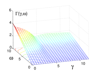
Figure 2: (Color online)An illustration of $\Gamma=\Gamma(\gamma,\omega)$ as a function of $\omega$ and $\gamma$. $\omega$ was chosen in units of $\mu B_{0}$, and this plot is for $\theta=\frac{1}{4}\pi$.

The numerical results of $\Gamma(\gamma,\omega)$ versus $\gamma$ and $\omega$ were illustrated in figure 1. The rotating frequency $\omega$ of the driven field was plotted in units of $\mu B_{0}$, where $B_{0}$ is the modulus of the driving field. Figure 1 shows us that $\Gamma(\gamma,\omega)$ depends on $\omega$ linearly with a fixed $\gamma$, while $\Gamma(\gamma,\omega)$ decreases with $\gamma$ increasing. This can be understood as the following. Without the driving field $\vec{B}(t)$, the dependance of $|R_{m}(t)\rangle$ on $\gamma$ behaves like $e^{-\gamma t}$, while $\lambda_{m}$ depends on $\gamma$ linearly. Therefore, $\Gamma(\gamma,\omega)$ decays with $\gamma$ increasing and tends to zero when $\gamma\rightarrow\infty.$

V summary and discussion

We have presented an adiabatic approximation scheme for open systems. In contrast with the conventional adiabatic approximation, the adiabatic approximation for open systems have been defined as the adiabatic dynamics of a composite system, which consists of the system and an ancilla. Our effective-Hamiltonian based definition of adiabaticity retains the conventional adiabatic approximation in the ideal case of closed systems, hence it is of consistency. The definition of adiabaticity in open systems has been extended to a high-order adiabatic approximation, which was defined in accordance with an master equation for the rotated density matrix. The validity and invalidity condition of adiabticity has been derived and discussed. The violation of adiabatic evolution has been demonstrated by an field-driven dissipative spin-$\frac{1}{2}$ particle. The other applications and demonstrations such as geometric phase in open systems and the effect of decoherence on quantum adiabatic computing will be addressed elsewhere.

This work was supported by EYTP of M.O.E, NSF of China (10305002 and 60578014), and the NUS Research Grant No. R-144-000-071-305.

References

- (1) M. Born and V. Fock, Z. Phys. 51, 165 (1928).
- (2) L. D. Landau, Zeitschrift 2, 46 (1932); C. Zener, Proc. R. Soc. London Ser. A 137, 696 (1932).
- (3) M. Gell-Mann and F. Low, Phys. Rev. 84, 350 (1951).
- (4) M. V. Berry, Proc. R. Soc. London A 392, 45(1984).
- (5) P. Zanardi and M. Rasetti, Phys. Lett. A 264, 94 (1999).
- (6) J. A. Jones, V. Vedral, A. Ekert, and G. Castagnoli, Nature (London) 403, 869 (2000).
- (7) J. Pachos and S. Chountasis, Phys. Rev. A 62, 052318 (2000).
- (8) L.-M. Duan, J. I. Cirac, and P. Zoller, Science 292, 1695 (2001).
- (9) E. Farhi, J. Goldstone, S. Gutmann, and M. Sipser, e-print quant-ph/0001106.
- (10) E. Farhi, J. Goldstone, S. Gutmann, J. Lapan, A. Lundgren, and D. Preda, Science 292, 472 (2001).
- (11) M. S. Sarandy and D. A. Lidar, Phys. Rev. A 71, 012331(2005).
- (12) M. S. Sarandy and D. A. Lidar, Phys. Rev. Lett. 95, 250503(2005).
- (13) P. Thunström, J. Åberg, and E. Sjöqvist, Phys. Rev. A 72, 022328(2005).
- (14) C. W. Gardinar and P. Zoller, Quantum noise (Springer, Berlin, 2000).
- (15) X. X. Yi and S. X. Yu, J. Opt. B: Quantum Semiclass. 3, 372(2001).
- (16) B. A. Shadwick and W. F. Buell, J. Phys. A 34, 4771(2001).
- (17) B. Reznick, Phys. Rev. Lett. 76, 1192(1996).
- (18) A. R. P. Rau and R. A. Wendell, Phys. Rev. Lett. 89, 220405(2002).
- (19) A. V. Sokolov, A. A. Andrianov, and F. Cannata, e-print: quant-ph/0602207.
- (20) For recent progresses in this direction, please read, K. P. Marzlin, B. C. Sanders, Phys. Rev. Lett. 93, 160408(2004); D. M. Tong et al., Phys. Rev. Lett. 95 110407(2005). As shown, this condition may not be sufficient for some special systems, however, it is powerful in most cases. So does Eq.(13).
- (21) Degenerate levels are excluded.