Localization and its consequences
for quantum walk algorithms and quantum communication

Abstract

The exponential speed-up of quantum walks on certain graphs, relative to classical particles diffusing on the same graph, is a striking observation. It has suggested the possibility of new fast quantum algorithms. We point out here that quantum mechanics can also lead, through the phenomenon of localization, to exponential suppression of motion on these graphs (even in the absence of decoherence). In fact, for physical embodiments of graphs, this will be the generic behaviour. It also has implications for proposals for using spin networks, including spin chains, as quantum communication channels.

The starting point for the field of quantum computation is the realization that quantum algorithms may perform tasks more efficiently than known classical algorithms for the same problem Feynman . The first example of a complexity separation was discovered by Deutsch and Jozsa DeutschJozsa92 . Perhaps the most celebrated example is Shor’s factoring algorithm Shor94 , which is exponentially more efficient than any known classical algorithm.

A third class of quantum algorithms stem from random walks, which have proved a fruitful tool for finding classical algorithms ClassicalRandomWalkAlgorithms1 . And this has led to investigations of whether quantum random walks might offer additional benefit for producing fast algorithms. The first realization was that quantum random walks in one dimension propagate at a rate that is linear in time, compared to the square-root rate for classical random walks SquareRootSpeedUp . This already suggests that quantum walks may offer possibilities for at least polynomial speed-up of algorithms. Thus the subsequent discovery of quantum walks that are exponentially faster than classical walks is particularly striking and suggestive ChildsFarhi ; ExponentialSpeedUp ; Kempe05 .

The clear message is that quantum effects can enhance computation. In this paper we point out that the opposite is also possible and that quantum effects can cause exponential suppression of computations.

Our focus is on certain continuous time walks (in contrast to the discrete time “coined” walks mostly used in algorithmic applications) which, when carried out on ideally perfect quantum graphs, have exponentially faster propagation than a classical random walk on the same graph. We will apply well-established ideas from the theory of localization Anderson to these quantum walks to show that when the graphs have imperfections, as they surely will in any real physical implementation, the propagation of quantum information is suppressed exponentially in the amount of imperfection.

Our conclusion is that quantum walks on physical graphs are not likely to be useful for algorithmic purposes. It is worth stressing at this point, however, that applications of quantum walks in quantum algorithms are thought of as being simulated walks in the memory of a quantum computer – as is indeed always the case in the classical applications where the underlying graphs are typically exponentially large and hence would require exponential resources to realize physically.

Figure 1: The Graph ${\cal G}_{4}$ ChildsFarhi .

We describe in detail a particular example of propagation on a graph which, in the absence of imperfections, has the property that quantum evolution is exponentially faster than classical evolution; the effect of localization is particularly stark here. Later we point out the implications for quantum information processing tasks on other networks.

The particular case we will consider is the graph ${\cal G}_{n}$, first studied in ChildsFarhi . It consists of two joined branching trees with $2n+1$ vertical columns of nodes; ${\cal G}_{4}$ is illustrated in Figure 1. The question of interest is how rapidly a particle starting at the left-most node reaches the right-most node. Let us first describe the idea behind the exponential separation between classical diffusion and quantum motion on this graph (when the graph is perfect). Our treatment follows that in ChildsFarhi ; Kempe closely.

The model of classical diffusion is that the particle is equally likely to move from the node where it finds itself to any of the nodes to which it is linked. Explicitly we may take the motion to arise from the Markov transition matrix

$$M_{i,j}=\left\{\begin{array}[]{cl}-\gamma&\ i\neq j\mbox{ if nodes }i\mbox{ and }j\mbox{ connected}\\ 0&\ i\neq j\mbox{ if nodes }i\mbox{ and }j\mbox{ not connected}\\ d_{i}\gamma&\ i=j\end{array}\right.$$ (4)

where $\gamma$ is the constant jumping rate between two connecting vertices, and $d_{i}$ is the number of edges incident to the vertex $i$. The probability of being at node $i$ at time $t$ is governed by

$$\frac{dp_{i}(t)}{dt}=-\sum_{j}M_{i,j}p_{j}(t).$$ (5)

A classical particle finding itself in the middle of the graph (not at the left- or right-most node or one of the nodes precisely in the centre) is twice as likely to move towards the centre as away from it. Thus a classical particle starting at the left-most node will diffuse rapidly to the centre of the graph but then it will diffuse exponentially slowly from the centre of the graph to the rightmost node.

We now analyze the quantum walk on ${\cal G}_{n}$ ChildsFarhi starting in the state corresponding to the left-most node and evolving with the Hamiltonian given by

$$\left\langle a|H|b\right\rangle=M_{a,b},$$ (6)

where $\left|b\right\rangle$ represents the state of a particle at node $b$.

The key observation is that although there are exponentially many nodes, and a Hilbert space of exponential dimension, in fact the system only evolves in a $(2n+1)$-dimensional subspace. This subspace is spanned by states $|\tilde{j}\rangle$ (where $0\leq j\leq 2n$), the uniform superposition over all vertices in column $j$, that is,

$$|\tilde{j}\rangle=2^{-\min[j,2n-j]/2}\sum_{a\in\ {\rm column}\ {j}}|a\rangle.$$ (7)

In this basis, the non-zero matrix elements of $H$ are

$$\langle\tilde{j}|H|\tilde{j}\pm 1\rangle = -\sqrt{2}\gamma$$

$$\langle\tilde{j}|H|\tilde{j}\rangle = \left\{\begin{array}[]{ll}2\gamma&{j}=0,n,2n\\ 3\gamma&{\rm otherwise,}\\ \end{array}\right.$$ (10)

which is depicted in Figure 2 as a quantum random walk on a line with $2n+1$ vertices.

Figure 2: The elements of the Hamiltonian $H/{\gamma}$ for ${\cal G}_{4}$ when reduced to a walk on a line ChildsFarhi .

In particular it is seen that (away from the left-most or right-most vertices) the quantum particle has equal amplitude to move to the left as to the right, and in particular it is not exponentially suppressed from moving right once it has reached the centre. (Observe that the central node, coming from the centre of the graph ${\cal G}_{n}$, has a special status, but that will us not concern here.)

We now turn to the main point of this paper. If we were to try and build this graph physically and get a quantum particle to evolve on it, it would be virtually impossible to do so perfectly. In particular, for example, the distances between the nodes will inevitably vary slightly from edge to edge. Our main observation will be that the theory of Anderson localization Anderson implies that this variability will lead to suppression of the quantum evolution so that in fact a quantum particle starting at the left of the graph can only travel a distance to the right proportional to an inverse power of the degree of variability. The probability of arriving at a point beyond this “localization length” is exponentially small in the distance from the starting point. Thus if the right-most node is further away than the localization length, the particle is effectively prevented from reaching it. We emphasize that localization is very much a quantum (or more strictly a wave) phenomenon; it does not affect classical particles diffusing. Indeed, Anderson localization is often characterized as the quantum suppression of classical diffusion. We feel it is striking that this is a case where quantum effects are suppressing rather than enhancing possibilities for information processing.

The imperfections in the quantum evolution we consider are within the graph itself; namely the Hamiltonian varies a little from node to node. But the evolution is unitary. In particular, we are not concerned with any interaction of the quantum system with the environment, in other words we assume that there is no decoherence DecoherenceInGraphs . In fact we will consider a rather weak model of imperfection for our graph. In the original $(2^{n+1}+2^{n}-2)$-node graph, one expects that the interaction connecting each pair of nodes will vary slightly from edge to edge. This breaking of the symmetry of the original system would have a substantial effect on the system, namely that the evolution would now no longer proceed simply through the states $\left|\tilde{j}\right\rangle$, but leak into the entire Hilbert space. Our model of the variability of the Hamiltonian is less severe than this: we assume that the evolution still proceeds through the states $\left|\tilde{j}\right\rangle$, but that this effective walk on the line is subject to a Hamiltonian that varies from node to node on the line. It is to be expected that the more general situation in which variability is allowed for all nodes/edges can only further suppress the quantum evolution. Thus our system is still considered to walk on a one-dimensional graph, but now our Hamiltonian is

$$H_{\epsilon}=H+\sum_{j}\epsilon_{j}\left|j\right\rangle\!\left\langle j\right|,$$ (11)

where $H$ is the Hamiltonian (Localization and its consequences for quantum walk algorithms and quantum communication). The variability is introduced via the parameters $\epsilon_{j}$. In the first instance the parameters $\epsilon_{j}$ will be taken independently from a Cauchy distribution with parameter $\delta$: the density is

$$P\left(\epsilon\right)=\frac{1}{\pi}\frac{\delta}{\epsilon^{2}+\delta^{2}}.$$ (12)

A particular reason for doing this is that the Cauchy distribution is most amenable to analytic treatment. Later we will point out that taking the $\epsilon_{j}$ to be chosen from other distributions makes no qualitative difference to the conclusions (although it does lead to some interesting quantitative differences). It will also be clear that we could encode variability in the Hamiltonian in various other ways than (11); for example the off-diagonal terms could have random components. Many studies in the localization literature DerridaGardner84 ; Slevin88 show that these possibilities do not make a qualitative change to our conclusion.

All our conclusions are encapsulated in Figure 3. The first plot shows the flow of intensity with time for motion along left half of the columns of ${\cal G}_{n}$ ($0<j<n$) according to the Hamiltonian (Localization and its consequences for quantum walk algorithms and quantum communication) - the perfect case. The signal clearly travels smoothly (and indeed at constant speed) along the chain. The remaining two plots show what happens when the Hamiltonian is now (11) with the $\epsilon_{j}$ taken from the Cauchy distribution with increasing amounts of variability, $\delta$. In all cases, we numerically computed the probability $\left|\left\langle{\tilde{j}}|\psi\left(t\right)\right\rangle\right|^{2}$ of a particle being in the state $\left|{\tilde{j}}\right\rangle$ for seven times $t$, where $\left|\psi\left(t\right)\right\rangle=\exp\left(-itH/\hbar\right)\left|\tilde{0}\right\rangle$, $\gamma=1$, $\hbar=1$, and $n=1000$.

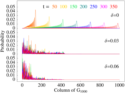
Figure 3: (Colour online) Propagation within the left side of ${\cal G}_{1000}$ at times $t$ according to; (top) the perfect Hamiltonian eq. (6), and the disordered Hamiltonian eq. (11) with (middle) disorder $\delta=0.03$, and (bottom) disorder $\delta=0.06$.

When $\delta$ is non-zero, the quantum wave packet travels a certain distance along the graph, but is then seen to stop. The distance that the packet gets to is reduced as $\delta$ increases (in fact, as we shall see the distance is inversely proportional to $\delta$).

This behaviour is a classic example of Anderson localization Anderson . It arises since the eigenstates, $\left|E_{\alpha}\right\rangle$, of the Hamiltonian (11) are exponentially localized in space, rather than being extended into space as in the case (6). The modulus of the amplitude of each eigenstate is bounded by an exponential function

$$\left|\left\langle E_{\alpha}|{\tilde{j}}\right\rangle\right|<N_{\alpha}e^{-\left|{\tilde{j}}^{0}_{\alpha}-{\tilde{j}}\right|/{l_{\alpha}}},$$ (13)

where $l_{\alpha}$ is the localization length and $N_{\alpha}$ is a normalization constant. It is simple to see why this behaviour of the eigenstates causes the time evolution witnessed in Figure 3. The state of the system at time $t$ may be written as

$$\left|\psi(t)\right\rangle=\sum_{\alpha}\psi_{\alpha}e^{-itE_{\alpha}/\hbar}\left|E_{\alpha}\right\rangle,$$ (14)

where $\psi_{\alpha}=\langle{E_{\alpha}}\left|\psi(0)\right\rangle$ are the amplitudes of the initial state and $E_{\alpha}$ are the energy levels. Now consider a quantum state initially concentrated at some point. This initial state will only have substantial amplitude in energy eigenstates which are localized in regions close to that initial point. As the state evolves with time, the phase of these amplitudes can change, but not the modulus of the amplitudes. Thus for all time the state is expanded in terms of states which have small amplitude far from the initial point.

For the particular model of Hamiltonian variability (11), we can explicitly describe the behaviour of the localization length of eigenstates as $\delta$ varies, treating as negligible the influence of the anomalous end and centre points of the graph. Namely, it has then been shown LloydThouless that

$$\cosh{\frac{1}{l_{\alpha}}}=\frac{\sqrt{\left(\!\sqrt{8}\gamma\!+\!\hat{E}_{\alpha}\right)^{2}\!\!+\!\delta^{2}}\!+\!\sqrt{\left(\!\sqrt{8}\gamma\!-\!\hat{E}_{\alpha}\right)^{2}\!\!+\!\delta^{2}}}{\sqrt{32}\gamma},$$ (15)

where $\hat{E}_{\alpha}=E_{\alpha}-3\gamma$. It is not difficult to check that the largest localization length occurs for $E_{\alpha}=3\gamma$, and for small $\delta$ (i.e. $\delta\ll\sqrt{8}\gamma$) it becomes $l_{\rm max}\sim\sqrt{8}\gamma/\delta$. Since the Hamiltonian has a random component, it will almost surely not have an eigenvalue equal to $3\gamma$; but the localization length for $E_{\alpha}=3\gamma$ is an upper bound for the localization length of any eigenstate. And hence this gives an estimate of the furthest distance a signal starting at a given point will get to. The plots in Figure 3 bear this out.

This then is the main conclusion of our investigation. A particularly quantum effect, Anderson localization, causes a particle undergoing a quantum walk in the graph to be effectively stopped from propagating from left to right. More precisely, consider a fixed value of the degree of variability $\delta$, and a series of graphs ${\cal G}_{n}$ with $n$ increasing. Once the length of the graph $n$ is greater than about the maximum localization length $\sqrt{8}\gamma/\delta$, the probability of the particle reaching the right-most node, having started at the left-most node is exponentially small in $n$.

This is reminiscent of the behaviour of the classical random walk on the same graph. However it is fundamental that the exponents arise from quite different sources. In particular we note that in the original problem of motion on the graph ${\cal G}_{n}$, a classical particle diffusing from left to right travels rapidly from the left most node to the centre, and the exponential time it takes to get from left to right arises from the fact that it is difficult to get from the centre of the graph to the right-most node. In the case of a quantum particle on an imperfect graph, localization means that it can be exponentially difficult even to get from the left-most node to the centre of the graph.

It is important to point out that localization is not a consequence of our choice of Cauchy distributed disorder. It is a generic property of disordered systems, in one dimension, occurring for any distribution. For other choices (e.g Gaussian or uniform on an interval), the qualitative features are the same as for the Cauchy case, but the quantitative details may differ; in particular, if $P(\epsilon)$ has a second moment, the localization length typically scales like $\delta^{-2}$ as $\delta\rightarrow 0$, rather than $\delta^{-1}$ DerridaGardner84 .

The graph ${\cal G}_{n}$ is of particular interest because of its relationship to quantum algorithms and the exponential separation between between classical and quantum propagation. However our results also have implications for other quantum information processing tasks. For example, there has been considerable interest recently in using spin chains and other networks for propagation quantum information spinchains . The message of this paper is that localization will present a fundamental difficulty for these proposals even in the absence of external interactions with the system. (See also deChiara .)

To end this discussion, we emphasise two differences of the model considered here to noisy quantum computation. First, noise in quantum computers is usually modelled as sufficiently independent stochastic variations in the dynamics, in particular on a single memory qubit they vary with time; here, we have randomness in the description of the system itself, i.e. the Hamiltonian, but on the other hand the localization effect remains even if the particular random Hamiltonian is known. Second, we consider here free evolution of the quantum state on a spatially extended system; this means that any comparison with quantum computers should not be with the circuit model (for which also techniques for fault-tolerant computation exist fault-tolerant ), but rather with computation in a closed system, like quantum cellular automata qca . It is not known whether fault-tolerant techniques for universal quantum cellular automata in one dimension apply to the type of error considered in localization: fault-tolerant computing usually has to assume a degree of independence of errors, both spatially and in time, and although able to cope with certain correlations, the persistent “failure” of an interaction in always the same way throughout the evolution seems to present a new challenge.

Also, it should be pointed out that localization is known to occur for a single spin excitation moving in spin lattices, and it may be expected for small numbers of excitations; however, universal quantum computation happens in the regime of many excitations, where it is not known if localization presents an obstacle for information propagation.

We remark finally that the systems we have considered here are different to stroboscopic ($\delta$-kicked) models (e.g. those in BuerschaperBoness ) which are closely related to the kicked rotor, where localization occurs for quantum chaotic reasons Fishman82 , and its consequences have been extensively explored by Shepelyansky and co-workers (see for example Shepelyansky01 ).

- (1) R. P. Feynman, Int. J. Theor. Phys. 21 467 (1982).
- (2) D. Deutsch, and R. Jozsa, Proc. Roy. Soc. Lond. A 439, 553 (1992).
- (3) P. W. Shor, in Proc. 35th FOCS, IEEE Computer Society, Los Alamitos, CA, 124-134 (1994).
- (4) R. Motwani, and P. Raghavan, Randomized Algorithms, (Cambridge University Press, Cambridge, 1995)
- (5) D. Aharonov, et al., in Proc. 33rd STOC, New York, ACM, 50-59 (2001); A. Ambainis, et al., in Proc. 33rd STOC, New York, ACM, 60-69 (2001).
- (6) A. Childs, E. Farhi and S. Gutmann, Quantum Information Processing, 1, 35 (2002).
- (7) A. M. Childs, et al., in Proc. 35th STOC, 59-68 (2003).
- (8) J. Kempe, Prob. Theory and Rel. Fields, 133, 215 (2005).
- (9) P. W. Anderson, Phys. Rev. 109, 1492 (1958).
- (10) J. Kempe, Contemp. Phys. 44, 307 (2003).
- (11) D. Solenov and L. Fedichkin, Phys. Rev. A 43, 012313 (2006). T. Brun, H. Carteret and A. Ambainis, Phys. Rev. A 67, 032304 (2003). V. Kendon and B. Tregenna, Phys. Rev. A 67, 042315 (2003).
- (12) B. Derrida and E. Gardner, J. Phys. Paris 45, 1283-1295 (1984); L. Pastur and A. Figotin, Spectra of Random and Almost-Periodic Operators, (Berlin Heidelberg, Springer Verlag, 1992).
- (13) K. M. Slevin, J. B. Pendry, J. Phys. C. 21, 141 (1988).
- (14) P. Lloyd, J. Phys. C 2, 1717 (1969); D. J. Thouless, J. Phys. C 5, 77 (1972)
- (15) S. Bose, Phys. Rev. Lett. 91, 207901 (2003); T. J. Osborne and N. Linden, Phys. Rev. A. 69, 052315 (2004); M. Christandl, et. al., Phys. Rev. A 71, 032312 (2005).
- (16) G. De Chiara, D. Rossini, S. Montangero, R. Fazio, Phys. Rev. A 72, 012323 (2005).
- (17) P. W. Shor, in Proc. 37th FOCS, IEEE Computer Society, Los Alamitos, CA, 56-65 (1996); D. Aharonov and M. Ben-Or, in Proc. 29th STOC, 176-188 (1997); quant-ph/9906129 (1999).
- (18) B. Schumacher, R. F. Werner, quant-ph/0405174 (2004).
- (19) O. Buerschaper and K. Burnett, quant-ph/0406039 (2004); T. Boness, S. Bose and T. S. Monteiro, Phys. Rev. Lett. 96, 187201 (2006).
- (20) S. Fishman, D. R. Grempel, R. E. Prange, Phys. Rev. Lett. 49 509 (1982).
- (21) D. L. Shepelyansky, Physica Scripta, T90, 112 (2001).