A Bell pair in a generic random matrix environment

Abstract

Two non-interacting qubits are coupled to an environment. Both coupling and environment are represented by random matrix ensembles. The initial state of the pair is a Bell state, though we also consider arbitrary pure states. Decoherence of the pair is evaluated analytically in terms of purity; Monte Carlo calculations confirm these results and also yield the concurrence of the pair. Entanglement within the pair accelerates decoherence. Numerics display the relation between concurrence and purity known for Werner states, allowing us to give a formula for concurrence decay.

The evolution of entanglement within a pair of qubits or spin $1/2$ particles under the influence of an environment is paradigmatic for the stability of teleportation spe , and indeed for any quantum information process Nielsen and Chuang (2000). Concurrence provides a measure for the degree of entanglement within such a pair Hill and Wootters (1997). The main purpose of the present paper is to establish the generic behavior of the decay of entanglement, i.e. concurrence, of such a pair of qubits. We propose a random matrix model for the unitary evolution of a pair of qubits interacting with one or two environments, but not among themselves. The environment(s) as well as the couplings will be described by one of the classical ensembles of random matrices Cartan (1935). Research in ”quantum chaos” has revealed, that such ensembles describe a chaotic environment well Guhr et al. (1998); Muller et al. (2005) and relations to the Caldeira-Legget model have been established Lutz and Weidenmueller (1999). In the present article we shall concentrate on the Gaussian unitary ensemble (GUE), which describes time-reversal breaking dynamics, mainly because it provides the simplest analytics. The model we use is based on one developed in general for the evolution of decoherence Gorin and Seligman (2002) and applied to fidelity decay Gorin et al. (2004); the latter was successfully tested by experiment R. Schäfer et al. (2005a, b); Gorin et al. (2006). We shall also need information about the evolution of the entanglement of the pair with the environment i.e. of its decoherence. This we measure in terms of purity Zurek (1991) rather then von Neumann entropy, because the analytic structure of purity allows an analytic treatment in terms of a Born expansion. Using this expression we see that purity of an entangled state decays faster than purity of a product state, but we shall be able to go one step further. Numerically we show that the relation of purity to concurrence demonstrated for a specific dynamical model Pineda and Seligman (2006) is universal, in the sense that it holds for the random matrix model. This relation coincides with the one for a Werner state and thus is analytically known, allowing us to give a closed, though heuristic, expression for concurrence decay. Both quantities and thus their relation are acessable by quantum tomography in experiments with trapped ions or atoms, whereinteraction with a controled environment is feasable bla .

Concurrence of a density matrix $\rho$ representing the state of a pair of qubits, is defined as

$$C(\rho)=\max\{0,\lambda_{1}-\lambda_{2}-\lambda_{3}-\lambda_{4}\}$$ (1)

where $\lambda_{i}$ are the eigenvalues of the matrix $\sqrt{\rho(\sigma_{y}\otimes\sigma_{y})\rho^{*}(\sigma_{y}\otimes\sigma_{y})}$ in non-increasing order; $(^{*})$ denotes complex conjugation in the computational basis and $\sigma_{y}$ is a Pauli matrix. Purity is defined as

$$P(\rho)={\text{Tr}}\rho^{2}.$$ (2)

We study dynamics on a Hilbert space with the structure ${\mathcal{H}}\ =\ {\mathcal{H}}^{\textrm{q}}_{1}\otimes{\mathcal{H}}^{\textrm{e}}_{1}\otimes{\mathcal{H}}^{\textrm{q}}_{2}\otimes{\mathcal{H}}^{\textrm{e}}_{2}$, where ${\mathcal{H}}^{\textrm{q}}_{i}$ indicates (two dimensional) qubit spaces, while ${\mathcal{H}}^{\textrm{e}}_{i}$ will indicate $N$ dimensional environments.

We consider unitary dynamics on the entire space and obtain the non-unitary dynamics for the qubits by partial tracing over the environment(s). As we wish to consider the effect of the environment on the pair of qubits, we cannot allow any interaction within the pair, but we consider interactions with the environments, which may be fused to a single one. For convenience we also neglect any possible evolution for each qubit individually, which is not induced by the coupling to the environment. The latter is non-essential to our argument, but simplifies the analytic treatment. We thus use the Hamiltonian

$$H=H_{1}^{\textrm{e}}+H_{2}^{\textrm{e}}+\lambda_{1}V_{1}^{{\textrm{e}},{\textrm{q}}}+\lambda_{2}V_{2}^{{\textrm{e}},{\textrm{q}}}.$$ (3)

The first two terms correspond to dynamics of the environments. The third and fourth terms represent the coupling of each of the qubits to the corresponding environment. To obtain further simplification, we consider one of the qubits as a spectator, i.e. we assume that it has no coupling to an environment ($\lambda_{2}=0$). The corresponding environment becomes irrelevant and we obtain the simplified Hamiltonian

$$H_{\lambda}=H^{\textrm{e}}_{1}+\lambda V^{{\textrm{e}},{\textrm{q}}}_{1}.$$ (4)

Note that we do consider entanglement with the spectator. This yields the simplest Hamiltonian for which we can analyze the effect of an environment on a Bell pair. The environment Hamiltonian $H^{\textrm{e}}_{1}$ will be chosen from a classical ensemble Cartan (1935) of $N\times N$ matrices and the coupling, $V^{{\textrm{e}},{\textrm{q}}}_{1}$, from one of $2N\times 2N$ matrices. As usual, the GUE ensemble, which represents time-reversal invariance breaking dynamics, is easier to handle analytically than the Gaussian orthogonal one. Here we focus on the former, while treating the latter in a follow up paper. Evolution of both purity and concurrence of the pair of qubits can readily be simulated in a Monte Carlo calculation and due to the simple structure of purity, it is possible to compute analytically this quantity in linear response approximation. An exact calculation requires four-point functions, which despite of the power of super-symmetric techniques Guhr et al. (1998) are still not readily available.

To calculate the value of purity, we use the following averages and approximations. First we expand the evolution operator as a Born series; hence we require small $\lambda$ and/or short times. We average both $V_{1}^{{\textrm{e}},{\textrm{q}}}$ (which will be called $V$ from now on) and $H^{\textrm{e}}_{1}$ over the appropriate GUE ensemble. Finally we average the initial state and obtain Eq. (12). This is the very same scheme followed in Gorin et al. (2004) for fidelity decay, though details are more complicated Gorin and Seligman (2002) due to the partial traces.

We define the evolution operator $U_{\lambda}=\exp[-\imath H_{\lambda}t]$, such that the density matrix in Eqs. (1) and (2) is $\rho(t)={\text{Tr}}_{\text{env}}U_{\lambda}|\psi(0)\rangle\langle\psi(0)|U_{\lambda}^{\dagger}$, where $|\psi(0)\rangle$ is the initial state of the system. Since $U_{0}$ is a local operation in the environment it will not affect the value of $\rho$. Thus we can equally evolve with $U_{0}^{\dagger}U_{\lambda}$ instead of $U_{\lambda}$ alone. It is convenient to use $U_{0}^{\dagger}U_{\lambda}$ since for small $\lambda$ this operator will remain in some sense near to unity for longer times. We write the Born series to second order as

$$U_{0}^{\dagger}\,U_{\lambda}\approx\openone-\imath\lambda I(t)-\lambda^{2}J(t);$$ (5)

$$I(t)=\int_{0}^{t}\text{d}\tau\tilde{V}(\tau);\,J(t)=\int_{0}^{t}\text{d}\tau\int_{0}^{\tau}\text{d}\tau^{\prime}\tilde{V}(\tau)\tilde{V}(\tau^{\prime}).$$ (6)

Here $\tilde{V}(t)$ is the coupling operator in the interaction picture: $\tilde{V}(t)=U_{0}^{\dagger}VU_{0}$. Writing $|\psi(0)\rangle=\sum_{\mu=1}^{4N}x_{\mu}|\mu\rangle$, and using Eq. (5), purity reads as:

$$P(t)\approx 1-\lambda^{2}(\text{Re}A_{J}-A_{1}-A_{2}+\text{Re}A_{3});$$ (7)

$$A_{J} =4x_{\mu}x_{i^{\prime}jk}^{*}x_{i^{\prime}j^{\prime}k^{\prime}}x_{ij^{\prime}k^{\prime}}^{*}J_{ijk,\mu}(t),$$ (8a)

$$A_{1} =2x_{\mu}x_{\nu}^{*}x_{i^{\prime}j^{\prime}k^{\prime}}x_{ij^{\prime}k^{\prime}}^{*}I_{ijk,\mu}(t)I_{i^{\prime}jk,\nu}^{*}(t),$$ (8b)

$$A_{2} =2x_{\mu}x_{i^{\prime}jk}^{*}x_{i^{\prime}j^{\prime}k^{\prime}}x_{\nu}^{*}I_{ijk,\mu}(t)I_{ij^{\prime}k^{\prime},\nu}^{*}(t),$$ (8c)

$$A_{3} =2x_{\mu}x_{i^{\prime}jk}^{*}x_{\nu}x_{ij^{\prime}k^{\prime}}^{*}I_{ijk,\mu}(t)I_{i^{\prime}j^{\prime}k^{\prime},\nu}(t)$$ (8d)

(summation over repeated indices is assumed). Indices run as follows: Greek ones over the whole Hilbert space, the $i$’s over the environment, $j$’s over the first qubit and $k$’s over the spectator qubit. Note that we use the natural notation for the indices of vectors in a space which is a tensor product of several spaces.

We now average the perturbation $V$ over the GUE using $\left\langle V_{m,n}\right\rangle=0$ and $\left\langle V_{m,m^{\prime}}V_{n,n^{\prime}}\right\rangle=\delta_{m,n^{\prime}}\delta_{m^{\prime},n}$. Due to the unitary invariance of the GUE we choose the basis that diagonalizes $H^{\textrm{e}}_{1}$ yielding eigenvalues $E_{i}$. Then

$$\langle J(t)\rangle_{ijk,i^{\prime}j^{\prime}k^{\prime}}=2\delta_{ijk,i^{\prime}j^{\prime}k^{\prime}}\\ \times\int_{0}^{t}\text{d}\tau\int_{0}^{\tau}\text{d}\tau^{\prime}\sum_{i^{\prime\prime}}e^{\imath(\tau^{\prime}-\tau)(E_{i^{\prime\prime}}-E_{i})}.$$ (9)

The matrix elements of the tensors $I\otimes I$ and $I\otimes I^{*}$, averaged, yield

$$\langle I_{ijk,lmn}(t_{1})I_{i^{\prime}j^{\prime}k^{\prime},l^{\prime}m^{\prime}n^{\prime}}(t_{2})\rangle$$

$$\quad=-\langle I_{ijk,lmn}(t_{1})I_{l^{\prime}m^{\prime}k^{\prime},i^{\prime}j^{\prime}n^{\prime}}^{*}(-t_{2})\rangle$$

$$\quad=\delta_{ijk,l^{\prime}m^{\prime}n}\delta_{i^{\prime}j^{\prime}k^{\prime},lmn^{\prime}}\int_{0}^{t_{1}}\text{d}\tau\int_{0}^{t_{2}}\text{d}\tau^{\prime}e^{\imath(E_{i}-E_{l})(\tau-\tau^{\prime})}.$$

Next we average $H^{\textrm{e}}_{1}$ over the GUE using that $\langle\sum_{i,i^{\prime}}e^{\imath(E_{i}-E_{i^{\prime}})t}\rangle=N[1+\delta(t/\tau_{H})-b_{2}(t/\tau_{H})]$, where $b_{2}(t/\tau_{H})$ is the form factor of the GUE Guhr et al. (1998) and $\tau_{H}$ the Heisenberg time, set to $2\pi$ throughout this letter.

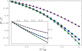
Figure 1: We show the evolution of purity for separable states (purple triangles), Bell states (green circles) and concurrence for Bell states (blue squares) in the crossover regime. The lines show theoretical predictions given by Eqs.(13) and (14). The environment has dimension $2^{10}$ and the perturbation strength is $\lambda=0.025$. In the inset we observe the Fermi golden rule regime for a larger perturbation $\lambda=0.1$.

The initial state is a product of pure states for the qubit pair and the environment. For the latter we use a random initial state $\sum_{i}x_{i}|i\rangle$, constructed in the large $N$ limit, using complex random numbers $x_{i}$ distributed according to a Gaussian centered around zero with width $1/\sqrt{N}$. For the pair of qubits we choose a completely general pure state. Since we still have the freedom to perform an arbitrary unitary local operation on each qubit, we pick a basis in which the initial state for the two qubits is

$$|\varphi_{\alpha}\rangle=\cos\alpha|00\rangle+\sin\alpha|11\rangle,\,\alpha\in[0,\pi/4].$$ (10)

The degree of entanglement is characterized by $\alpha$; in fact $C(|\varphi_{\alpha}\rangle\langle\varphi_{\alpha}|)=\sin 2\alpha$. Hence our initial state can be written as $|\psi(0)\rangle=\sum_{i}x_{i}|i\rangle|\varphi_{\alpha}\rangle$. Neglecting higher order terms in $1/N$, we obtain $\langle\langle A_{J}\rangle\rangle=2f(t)$ and $\langle\langle A_{2}\rangle\rangle=g_{\alpha}f(t)$ with

$$f(t)=\begin{cases}2t\tau_{h}+\frac{2t^{3}}{3\tau_{h}}&\text{if $0\leq t<\tau_{H}$}\\[5.69046pt] 2t^{2}+\frac{2\tau_{h}^{2}}{3}&\text{if $t\geq\tau_{H}$},\end{cases}$$ (11)

and $g_{\alpha}=\cos^{4}\alpha+\sin^{4}\alpha$. To leading order $\langle\langle A_{1}\rangle\rangle=\langle\langle A_{3}\rangle\rangle=0$. We obtain

$$P_{\textrm{LR}}(t)=1-\lambda^{2}(2-g_{\alpha})f(t).$$ (12)

From this result we see directly that purity decay will be faster the more entangled the initial state was. The validity of this approximation is limited to large values of purity, i.e. short times or weak coupling. This is valuable for applications to quantum information, but we are interested in the dynamical picture as a whole and thus would like to obtain an expression valid for a wide range of physical situations. As a way to achieve this for fidelity decay, exponentiation of the leading term of the linear response formula was proposed Prosen and Seligman (2002). A similar approximation is taken here, to obtain $P_{\textrm{ELR}}(t)$. In order to calculate the appropriate formula, we must satisfy $P_{\textrm{ELR}}(t)\approx P_{\textrm{LR}}(t)$ for small $t$, and consider correct asymptotics. These will be estimated as the purity after applying a totally depolarizing channel on one qubit to the 2 qubit state Eq. (10). The expected asymptotic value is $g_{\alpha}/2$, and the final expression is

$$P_{\textrm{ELR}}(t)=\frac{g_{\alpha}}{2}+\left(1-\frac{g_{\alpha}}{2}\right)e^{\frac{P_{\textrm{LR}}(t)-1}{1-g_{\alpha}/2}}.$$ (13)

This result is in excellent agreement with numerics as shown in Fig. 1, and displays the transition from exponential to Gaussian decay as Heisenberg time is reached.

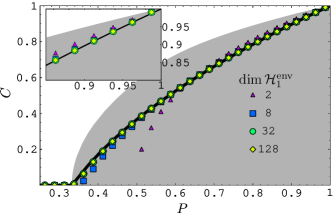
Figure 2: The relation between $C$ and $P$ for a fixed coupling ($\lambda=0.3$) and variable size of the environment. We average over 10 realizations of the Hamiltonian (4) and 15 initial conditions. The gray area indicates the region of physical states, and the line the concurrence-purity relation for Werner states. In the inset we observe short time deviations from this relation.

We thus have an approximate formula for the decay of purity of a Bell pair. What about concurrence? At this point we take up a result Pineda and Seligman (2006) for the behavior of a Bell pair coupled to a kicked spin chain Prosen (2002). For a wide range of situations the decay of a pure Bell state leads to purities and concurrences that closely follow those of a Werner state in a Concurrence-Purity (CP) diagram Pineda and Seligman (2006). To test model independence, and thus universality of this behavior we make the corresponding numerical simulations in the RMT model. We find that the Werner state CP relation is quite well fulfilled in the large $N$ limit, as can be seen in Fig. 2, where results for fixed coupling but different sizes of the RMT environment are shown. Studying other couplings allowed by the full Hamiltonian Eq. (3) leads to similar results even if we are in different purity decay regimes. A partial explanation for this behavior can be found in Ziman and Buzek (2005).

We thus have the second relevant result of this paper; namely the relation of purity to concurrence for a non-interacting Bell pair interacting with a chaotic environment follows generically the curve of a Werner state. The importance of this statement is underlined by the fact, that the actual state reached at any time is typically not a Werner state. This is tested, by considering the spectrum of the density matrix, which should display a triple degeneracy for a Werner state. In fact a typical spectrum at $P=0.51$ is $\{0.692,0.142,0.110,0.056\}$.

Having established the genericity of the Werner state relation we can now insert the expression (13) for purity into the latter and obtain the heuristic expression

$$C_{\textrm{ELR}}(t)=\max\left\{0,\frac{\sqrt{12P_{\textrm{ELR}}(t)-3}-1}{2}\right\}$$ (14)

for concurrence decay. In Fig. 3 we can see that this relation is well obeyed by Monte Carlo calculations. Here we obtain two different time regimes, an exponential one (Fermi golden rule) for strong perturbations and a Gaussian one for weak perturbation. The time scale which defines the crossover between the two regimes is the Heisenberg time of the environment. Since the exponential behavior can be obtained letting the Heisenberg time go to infinity, we retrieve results derived from a master equation approach F. Mintert et al. (2005).

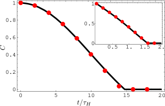
Figure 3: The average evolution of concurrence using and environment of dimension 128 and averaging over 10 Hamiltonians and 15 initial conditions is shown. The black curve corresponds to Eq. (14). We show both the Gaussian regime ($\delta=0.008$) and the Fermi golden rule regime in the inset ($\delta=0.07$).

We have thus obtained a satisfactory expression for concurrence decay, but we have to remember that we used an extremely simplified model. In some points the linear response treatment of the RMT model is slightly affected by these assumptions; we have made calculations where these approximations where lifted. In other words we have allowed both qubits to interact, either with independent environments or with the same one, see Eq. (3). The form of our result is essentially the same:

$$P_{\textrm{LR}}(t)=1-(2-g_{\alpha})[\lambda_{1}^{2}f_{1}(t)+\lambda_{2}^{2}f_{2}(t)],$$ (15)

where $f_{i}(t)$ is identical to $f(t)$ as in Eq. (11), but using the Heisenberg time of $H_{i}^{\textrm{e}}$. Other generalizations are possible. Local Hamiltonians for each qubit causing the degeneracy of the levels of the qubits to be lifted can be included. Environment Hamiltonians and couplings chosen from the Gaussian orthogonal ensemble may also be considered, as well as mixed states for the environment. Detailed linear response calculations as well as Monte Carlo calculations for these cases will be presented in the follow up paper.

Some points are worth mentioning: a) We see significant deviations from the usual exponential decay at times of the order of the Heisenberg time as defined by the environment. Thus, if the spectrum of the environment becomes very dense, and correspondingly the Heisenberg time moves off to infinity we recover the usual stochastic result. b) If the transition region can actually be seen, then the spectral stiffness of a chaotic environment has a small but significant stabilizing effect. The absence of spectral stiffness can be modeled by the so-called Poisson random ensemble Dittes et al. (1991). c) We have limited our discussions to the GUE for two reasons. The simple form of the form factor yields a concise final expression for purity decay. An additional advantage resulting from the unitary invariance of the coupling term, is that the final result is invariant under any local operation at each qubit. This is no longer guaranteed for orthogonal invariance only. The implications will be discussed in another paper.

Summarizing, we have developed a random matrix model for the evolution of a Bell pair interacting with a generic chaotic environment. Within this model we derive the linear response approximation for the purity decay of a Bell pair and show that it differs significantly from decay of a product state of two spins or qubits, even in the extreme case, where one of the qubits is only a spectator. Exponentiation extends the validity of this result far beyond its original reach. Monte Carlo calculations show that the relation between concurrence and purity, as obtained for Werner states, holds for RMT models and we thus expect it to be generic. Based on these results we have obtained and tested a heuristic formula for the decay of concurrence of a non-interacting Bell pair.

- (1) M. Riebe et al., Nature 429, 734 (2004); M. D. Barrett et al., Nature 429, 737 (2004).
- Nielsen and Chuang (2000) M. A. Nielsen and I. L. Chuang, Quantum Computation and Quantum Information (Cambridge University Press, Cambridge, UK, 2000).
- Hill and Wootters (1997) S. Hill and W. K. Wootters, Phys. Rev. Lett. 78, 5022 (1997).
- Cartan (1935) È. Cartan, Abh. Math. Sem. Univ. Hamburg 11, 116 (1935).
- Guhr et al. (1998) T. Guhr, A. Mueller-Groeling, and H. A. Weidenmueller, Phys. Rep. 299, 189 (1998), eprint cond-mat/9707301.
- Muller et al. (2005) S. Muller, S. Heusler, P. Braun, F. Haake, and A. Altland, Phys. Rev. E 72, 046207 (2005).
- Lutz and Weidenmueller (1999) E. Lutz and H. A. Weidenmueller, Physica A 267, 354 (1999).
- Gorin and Seligman (2002) T. Gorin and T. H. Seligman, J. Opt. B 4, S386 (2002).
- Gorin et al. (2004) T. Gorin, T. Prosen, and T. H. Seligman, New J. of Physics 6, 20 (2004).
- R. Schäfer et al. (2005a) R. Schäfer et al., Phys. Rev. Lett. 95, 184102 (2005a).
- R. Schäfer et al. (2005b) R. Schäfer et al., New J. of Physics 7, 152 (2005b).
- Gorin et al. (2006) T. Gorin, T. H. Seligman, and R. L. Weaver, Phys. Rev. E 73, 015202(R) (2006).
- Zurek (1991) W. Zurek, Phys. Today 44, 36 (1991), eprint quant-ph/0306072.
- Pineda and Seligman (2006) C. Pineda and T. H. Seligman, Phys. Rev. A 73, 012305 (2006).
- (15) R. Blatt and H. Häffner, private communication.
- Prosen and Seligman (2002) T. Prosen and T. H. Seligman, J. Phys. A 35, 4707 (2002).
- Prosen (2002) T. Prosen, Phys. Rev. E 65, 036208 (2002).
- Ziman and Buzek (2005) M. Ziman and V. Buzek, Phys. Rev. A 72, 052325 (2005).
- F. Mintert et al. (2005) F. Mintert et al., Phys. Rep. 415, 207 (2005).
- Dittes et al. (1991) F.-M. Dittes, I. Rotter, and T. H. Seligman, Phys. Lett. A 158, 14 (1991).