Field autocorrelations in electromagnetically induced transparency: Effects of a squeezed probe field

Abstract

The interaction of a quantized field with three-level atoms in $\Lambda$ configuration inside a two mode cavity is analyzed. We calculate the stationary quadrature noise spectrum of the field outside the cavity in the case where the input probe field is in a squeezed state and the atoms show electromagnetically induced transparency (EIT). If the Rabi frequencies of both dipole transitions of the atoms are different from zero, we show that the output probe field have four maxima of squeezing absorption. We show that in some cases two of these frequencies can be very close to the transition frequency of the atom, in a region where the mean value of the field entering the cavity is hardly altered. Furthermore, part of the absorbed squeezing of the probe field is transfered to the pump field. For some conditions this transfer of squeezing can be complete.

I Introduction

Electromagnetically induced transparency (EIT) Harris (1997) is a technique that can be used to eliminate the fluorescence from an atom illuminated with light whose frequency is equal to a particular atomic transition. This phenomenon has been observed in systems of three-level atoms in $\Lambda$ configuration (see Fig. 1) Marangos (1998). In this configuration a mode of the field, called the pump field, interacts resonantly with one dipole transition, while another mode, the probe field, interacting with the second dipole transition, is tested for transparency. The maximum absorption of the probe field by the medium depends on the Rabi frequencies associated with each atomic optical transition. The maximum occurs for a detuning from resonance which increases monotonically with the Rabi frequencies. EIT has many applications such as ultra slow propagation Hau et al. (1999) and storage of light Liu et al. (2001), to name just a few.

In general, the mean value of the electromagnetic field after interacting with the medium is measured. We may wonder if the medium is also transparent to the field fluctuations of the initial incoming probe field, particularly if these fluctuations are due to an initial state of the field which does not have a classical analog, such as squeezed states. In order to further investigate this question it is necessary to treat the field quantum mechanically. Under the assumption that the pump field is classical and with Rabi frequency much larger than the associated Rabi frequency of the probe field treated quantum mechanically, Fleischhauer et. al. Fleischhauer and Lukin (2002) showed that the medium is transparent to the full quantum state. Furthermore they showed that they can transfer the state of the probe field to the atoms and then back to the field again. These results were partially confirmed by the experimental work of Akamatsu et. al. Akamatsu et al. (2004), where the transparency of the atoms was measured considering an initially squeezed vacuum state as a probe field. Recent experimental Alzar et al. (2003) Martinelli et al. (2004) Sautenkov et al. (2005) studies have shown how the noise of the probe field is influenced by the medium of $\Lambda$ systems in a parameter region where the atoms show electromagnetically induced transparency. Also theoretical work where the pump and probe fields are treated quantum mechanically Barberis-Blostein and Zagury (2004) Dantan and Pinard (2004) Dantan et al. (2005) Dantan et al. has recently been done. It turns out that when both modes, pump and probe, are in a coherent state, the medium is transparent for the initial fluctuations of the coherent state, except for expected fluorescence due to small absorption from the media when they are not in the totally ideal EIT situation Barberis-Blostein and Zagury (2004). Moreover, the effects of the field noise, particularly quantum noise and its influence on the atoms’ state has been investigated. Dantan et. al. Dantan and Pinard (2004) Dantan et al. (2005) have shown that an initially squeezed vacuum as a probe field can be transferred to the atomic ensemble. The situation where the Rabi frequency of the pump and probe field are comparable and the probe field is in a general squeezed state still lacks a complete theoretical treatment.

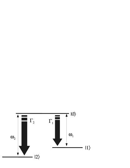
Figure 1: Atom in $\Lambda$ configuration, $\Gamma_{1}$ and $\Gamma_{2}$ represent radiative decaying constants.

In this paper we study the statistical properties of the electromagnetic quadrature functions of the stationary output field from a two mode cavity filled with three-level atoms in $\Lambda$ configuration. In particular we investigate the case when the two modes of the cavity field are in resonance with the dipole transitions of the three-level atoms and the corresponding interaction constants and decay rates are equal. For this case, when the mean value of the pump field is not zero the atoms show EIT and the average values of the field do not change during the interaction. We focus on the case where the input probe field does not have a classical analog, namely when it is in a squeezed state. The most interesting feature of the results for the quadrature noise spectrum is that, for a given frequency, close to the transition frequency of the atoms associated to the probe field, we have a maximum of absorption of the initial squeezing of the probe field. Remarkably, some of this initial squeezing of the probe field can be transferred to the pump field. This transfer is maximized when both Rabi frequencies are equal. The spectrum frequency where this transfer happens is very close to the resonance frequency of the probe field with the atom. Our results imply that the initial quantum properties of the fields are modified after interacting with the medium showing EIT.

This paper is organized as follows: in section II we give a brief review on how the system equations are obtained and solved. In section III we present the main new results, which consist of analytical expressions for the spectrum of the quadrature noise of the field after interacting with the medium when the Rabi frequency associated with each field is different from zero. Finally we present our conclusions in section IV.

II Cavity output field equations

Consider the case of $N$ three-level atoms in $\Lambda$ configuration inside a cavity that sustains two modes of the electromagnetic field. The frequencies of these modes are resonant with the transitions between levels $|1\rangle$ and $|0\rangle$ and $|2\rangle$ and $|0\rangle$ of the atom, respectively. The atoms are supposed to occupy a volume of small dimension as compared with the wavelength of the cavity modes. We point out that this is a difficult task to realize experimentally. The annihilation field operators for the modes inside the cavity are denoted by $\hat{a}_{1}$ and $\hat{a}_{2}$. We will work in the interaction picture, where the Hamiltonian of the cavity-atom interaction is given by

$$H_{\textrm{int}} = \sum_{j=1}^{N}\hbar(g_{1}\hat{\sigma}_{01}^{j}\hat{a}_{1}+g_{2}\hat{\sigma}_{02}^{j}\hat{a}_{2}+\textrm{c.c.}\,)$$ (1)

$$= \hbar g_{1}\hat{\Sigma}_{01}\hat{a}_{1}+\hbar g_{2}\hat{\Sigma}_{02}\hat{a}_{2}+\textrm{c.c.}\,,$$

where $\hat{\Sigma}_{ij}=\sum_{k=1}^{N}\hat{\sigma}_{ij}^{k}$ are the collective operators that represent the sum of individual atomic operators, $\sigma_{ij}^{k}=|i\rangle\langle j|^{k}$ associated with the $k^{\rm th}$ atom. We use input-output theory to relate the inside field with the outside field Walls and Milburn (1994). Each intra-cavity mode interacts with its own collection of modes in the outside field. This means that either they have different polarizations or their difference in frequency is large. The intracavity operators satisfy the equations

$$\frac{d}{dt}\hat{a}_{1}(t) = -ig_{1}\hat{\Sigma}_{10}(t)-\frac{\gamma_{1}}{2}\hat{a}_{1}(t)+\sqrt{\gamma_{1}}\,\hat{a}_{1{\rm in}}(t)\,,$$

$$\frac{d}{dt}\hat{a}_{2}(t) = -ig_{2}\hat{\Sigma}_{20}(t)-\frac{\gamma_{2}}{2}\hat{a}_{2}(t)+\sqrt{\gamma_{2}}\,\hat{a}_{2{\rm in}}(t)\,,$$ (2)

where $\gamma_{i}$ is the decay rate of cavity mode $i=1,2$. The operators $\hat{a}_{i{\rm in}}(t)=-1/\sqrt{2\pi}\int_{-\infty}^{\infty}d\omega e^{-i\omega(t-t_{0})}\hat{b}_{i}(t_{0},\omega)$ represent the field entering the cavity. The operator $\hat{b}_{i}(t_{0},\omega)$ represents the outside mode associated with cavity mode $i$ at the initial time $t_{0}$ and frequency $\omega$. We will call the outside field associated with the modes labeled by index $i=1$ ($i=2$) the pump (probe) field. In the interaction picture $\omega$ represents the detuning from the cavity frequency. The outcoming field is given by $\hat{a}_{i{\rm out}}(t)=1/\sqrt{2\pi}\int_{-\infty}^{\infty}d\omega e^{-i\omega(t-t_{1})}\hat{b}_{i}(t_{1},\omega)$. The operators $\hat{b}_{i}(t_{1},\omega)$ represents the outside mode associated with cavity mode $i$ at time $t_{1}>t_{0}$ and frequency $\omega$ Walls and Milburn (1994). The incoming and outcoming fields are related by

$$\hat{a}_{1{\rm in}}(t)+\hat{a}_{1{\rm out}}(t) = \sqrt{\gamma_{1}}\hat{a}_{1}(t)\,,$$

$$\hat{a}_{2{\rm in}}(t)+\hat{a}_{2{\rm out}}(t) = \sqrt{\gamma_{2}}\hat{a}_{2}(t)\,.$$ (3)

The Langevin equations for the atomic operators are obtained using the interaction Hamiltonian Eq. (1). Taking into account the interaction of the atom with modes other than the cavity in the usual way Orszag (2000), we obtain

$$\frac{d}{dt}\hat{W}_{1} = \frac{1}{3}(-2\Gamma_{1}-\Gamma_{2})(1+\hat{W}_{1}+\hat{W}_{2})-2ig_{1}\,\hat{\Sigma}_{01}\hat{a}_{1}$$ (4a)

$$+2ig_{1}\,\hat{\Sigma}_{10}\hat{a}_{1}-ig_{2}\,\hat{\Sigma}_{02}\hat{a}_{2}$$

$$+ig_{2}\,\hat{\Sigma}_{20}\hat{a}_{2}+\hat{F}_{W_{1}}\,,$$

$$\frac{d}{dt}\hat{W}_{2} = \frac{1}{3}(-\Gamma_{1}-2\Gamma_{2})(1+\hat{W}_{1}+\hat{W}_{2})-ig_{1}\,\hat{\Sigma}_{01}\hat{a}_{1}$$ (4b)

$$+ig_{1}\,\hat{\Sigma}_{10}\hat{a}_{1}-2ig_{2}\,\hat{\Sigma}_{02}\hat{a}_{2}$$

$$+2ig_{2}\,\hat{\Sigma}_{20}\hat{a}_{2}+\hat{F}_{W_{2}}\,,$$

$$\frac{d}{dt}\hat{\Sigma}_{10} = (-\frac{\Gamma_{1}+\Gamma_{2}}{2})\hat{\Sigma}_{10}+ig_{1}\,\hat{W}_{1}\hat{a}_{1}-ig_{2}\,\hat{\Sigma}_{12}\hat{a}_{2}+\hat{F}_{10}\,,$$

$$\frac{d}{dt}\hat{\Sigma}_{20} = (-\frac{\Gamma_{1}+\Gamma_{2}}{2})\hat{\Sigma}_{20}+ig_{2}\,\hat{W}_{2}\hat{a}_{2}-ig_{1}\,\hat{\Sigma}_{21}\hat{a}_{1}+\hat{F}_{20}\,,$$

$$\frac{d}{dt}\hat{\Sigma}_{21} = -ig_{1}\,\hat{\Sigma}_{20}\hat{a}_{1}^{\dagger}+ig_{2}\,\hat{\Sigma}_{01}\hat{a}_{2}\,,$$

where $\hat{W}_{j}=\hat{\Sigma}_{00}-\hat{\Sigma}_{jj}$ and $\hat{F}_{x}$ are collective Langevin operators given by the sum of each atom Langevin operator.

The Langevin fluctuation operators $\hat{F}$’s are assumed to be delta correlated, with zero mean:

$$\langle\hat{F}_{x}\rangle=0\,,$$ (5)

$$\langle\hat{F}_{x}(t)\hat{F}_{y}(t^{\prime})\rangle=D_{xy}\delta(t-t^{\prime})\,,$$ (6)

where $x$ and $y$ label the fluctuation operators.

The atom diffusion coefficients, $D_{xy}$, can be obtained using the generalized Einstein relations Cohen-Tannoudji et al. (1992). The nonzero diffusion coefficients are given by Eqs. (20) in appendix A.

We will consider the following initial condition for the incoming field. For frequencies different from the intra-cavity frequencies, for each mode of frequency $\omega$ associated to the field $i$, the field outside the cavity at time $t_{0}$ is given by $|\psi(t_{0},\omega)\rangle_{i}=\hat{S}(r_{i},\theta_{i})|0\rangle$, where $|0\rangle$ is the vacuum of the mode with frequency $\omega$ of the field $i$. The squeeze operator is given by $\hat{S}(r_{i},\theta_{i})=e^{1/2[\beta_{i}^{*}\,\hat{b}^{2}_{i}(t_{0},\omega)-\beta_{i}\,\hat{b}^{\dagger 2}_{i}(t_{0},\omega)]}$, with $\beta_{i}=r_{i}\exp{i\theta_{i}}$. When the frequency is equal to the intra-cavity frequency, the initial condition is: $|\psi(t_{0},\omega=0)\rangle_{i}=\hat{D}(\alpha_{i})\hat{S}(r_{i},\theta_{i})|0\rangle$, where $\hat{D}(\alpha_{i})=e^{\alpha_{i}\,\hat{b}^{\dagger}_{i}(t_{0},\omega)-\alpha_{i}^{*}\,\hat{b}_{i}(t_{0},\omega)}$ is the displacement operator which, when applied to the vacuum, creates the coherent state $|\alpha_{i}\rangle$. That means that the outside modes are initially in a vacuum, which can be squeezed, except for the resonant modes with the cavity which can be in a squeezed state but with field mean value different from zero. We will chose that value in a way such that inside the cavity we have $\langle\hat{a}_{i}\rangle=\alpha_{i}$.

Defining the field quadrature $\theta$ for the field $i$ and frequency $\omega$ as

$$\hat{Y}_{i\,\theta}(\omega,t)=\hat{b}_{i}(\omega,t)\exp{(i\theta)}+\hat{b}^{\dagger}_{i}(\omega,t)\exp{(-i\theta)}\,,$$ (7)

we have that the $\theta$-quadrature noise operator is given by

$$\Delta Y_{i\,\theta_{i}}(\omega,t=t_{0})=\langle(\hat{Y}_{i\,\theta_{i}}(\omega,t_{0})-\langle\hat{Y}_{i\,\theta_{i}}(\omega,t_{0})\rangle)^{2}\rangle=e^{-2r_{i}}\,,$$

for the given initial conditions.

Writing $\sqrt{\gamma_{i}}\,\hat{a}_{i\,{\rm in}}=\sqrt{\gamma_{i}}\,\langle\hat{a}_{i\,{\rm in}}\rangle+\hat{f}_{ai}$, one can show that for the initial conditions given above, the operators $\hat{f}^{\dagger}_{ai}(t)$ satisfy

$$\langle\hat{f}^{\dagger}_{ai}(t)\hat{f}_{aj}(t^{\prime})\rangle = \gamma_{i}\,\sinh^{2}{r_{i}}\,\delta(t-t^{\prime})\delta_{ij}\,,$$

$$\langle\hat{f}_{ai}(t)\hat{f}^{\dagger}_{aj}(t^{\prime})\rangle = \gamma_{i}(\sinh^{2}{r_{i}}+1)\,\delta(t-t^{\prime})\delta_{ij}\,,$$

$$\langle\hat{f}^{\dagger}_{ai}(t)\hat{f}^{\dagger}_{aj}(t^{\prime})\rangle = -\gamma_{i}\cosh{r_{i}}\sinh{r_{i}}\exp{(-i\theta_{i})}\,\delta(t-t^{\prime})\delta_{ij}\,,$$

$$\langle\hat{f}_{ai}(t)\hat{f}_{aj}(t^{\prime})\rangle = -\gamma_{i}\cosh{r_{i}}\sinh{r_{i}}\exp{(i\theta_{i})}\,\delta(t-t^{\prime})\delta_{ij}\,.$$

From Eqs. (II) it is easy to see that $\hat{f}_{ai}$ represents the Langevin fluctuation operator associated with the mode $i$ inside the cavity.

Eqs. (II) and (4) are a set of first order nonlinear operator stochastic differential equations. To solve this system, it is usual to transform these equations into a system of c-number Ito stochastic differential equations. These new equations are equivalent to the original ones up to second order in the operators Davidovich (1996). Once we have c-number stochastic equations we can use normal stochastic methods to solve them Gardiner (1994). Since c-numbers commute, in order to perform this operation uniquely, we define an order for the operator, which we call “normal” order. The normal order we choose is

$$\hat{a}_{2}^{\dagger},\hat{a}_{1}^{\dagger},\hat{\Sigma}_{02},\hat{\Sigma}_{01},\hat{\Sigma}_{12},\hat{W}_{1},\hat{W}_{2},\hat{\Sigma}_{21},\hat{\Sigma}_{10},\hat{\Sigma}_{20},\hat{a}_{1},\hat{a}_{2}\,.$$ (9)

We will use the c-number variables $\Sigma_{ij}$, $W_{1}$, $W_{2}$, $\alpha_{i}^{\ast}$, $\alpha_{i}$ for the corresponding operators $\hat{\Sigma}_{ij}$, $\hat{W}_{1}$, $\hat{W}_{2}$, $\hat{a}_{i}^{\dagger}$, $\hat{a}_{i}.$ The stochastic average of a c-number variable is equal to the mean value of the corresponding operator and the stochastic average of the product of two c-number variables corresponds to the mean value of the normal ordered multiplication of the two corresponding operators. For example $\langle\Sigma_{02}(t)\Sigma_{12}(t^{\prime})\rangle_{st}=\langle\Sigma_{12}(t^{\prime})\Sigma_{02}(t)\rangle_{st}$ is equal to $\langle\hat{\Sigma}_{02}(t)\hat{\Sigma}_{12}(t^{\prime})\rangle$. Here $\langle\cdots\rangle_{st}$ means stochastic mean. Henceforth we will drop the subscript “st” in order to simplify the notation.

The new c-number equations for the system look the same as the operator equations except that we should replace the Langevin fluctuation operators by modified Langevin fluctuation forces. These modified Langevin fluctuation forces still have zero mean and are still delta function correlated. However, the diffusion coefficients associated to these new Langevin fluctuation forces are modified so that the operator equations of normal ordered products coincide with the c-number equations of the corresponding products. A very clear explanation of this procedure is given by L. Davidovich Davidovich (1996).

These new normal ordered diffusion coefficients satisfy the symmetry relation $D_{xy}=D_{yx}$. The non-zero coefficients (and the symmetrical ones) are given by Eqs. (LABEL:eq:cnumbercoe) in the appendix A.

We are mostly interested in the dynamics of fluctuations around the steady state. In order to calculate these dynamics, we express the solutions of the stochastic variables as the sum of the steady state value plus fluctuations. That is, for any stochastic variable $O,$ we write $O(t)\approx\langle O\rangle+\delta O(t),$ with $\delta O\ll\langle O\rangle.$ In the system equations, the atomic operators scale as the number of atoms, $N$, and the fluctuation forces scale as $\sqrt{N}$ Davidovich (1996). If the number of atoms inside the cavity is large enough ($N\gg 1$) the fluctuations are small and we can neglect terms of order higher than one in $\delta O.$ Neglecting those terms, we obtain to zeroth order, the equations for the mean values, which are solved for the stationary state in an analogous way to bistability problems. The corresponding differential equations for the fluctuations can be written in matrix form

$$\frac{d}{dt}\boldsymbol{\delta O}=\boldsymbol{B}\cdot\boldsymbol{\delta O}+\boldsymbol{G}\,,$$ (10)

where the column vectors $\boldsymbol{\delta O}$ and $\boldsymbol{G}$ have components

$$\boldsymbol{\delta O}^{T} = (\delta\alpha_{2}^{*},\delta\alpha_{1}^{*},\delta\Sigma_{02},\delta\Sigma_{01},\delta\Sigma_{12},\delta w_{1},\delta w_{2},\delta\Sigma_{21},\delta\Sigma_{10},$$

$$\delta\Sigma_{20},\delta\alpha_{1},\delta\alpha_{2}),$$

$$\boldsymbol{G}^{T} = (f_{\alpha 1}^{*},f_{\alpha 2}^{*},f_{02},f_{01},f_{12},f_{w_{1}},f_{w_{2}},f_{21},f_{10},$$

$$f_{20},f_{\alpha 1},f_{\alpha 2})\,.$$

The matrix $\boldsymbol{B}$ can be obtained from the expansion up to first order in $\delta O$ of the system’s dynamical equations in c-number representation. The stationary spectrum of the correlation of the c-numbers, $S_{ij}(\omega)=\int_{-\infty}^{\infty}d\tau\,e^{i\omega\tau}\langle O_{i}(t)O_{j}(t+\tau)\rangle$ can be written as Orszag (2000)

$$\langle\delta O_{i}(\omega)\delta O_{j}^{\ast}(\omega^{\prime})\rangle=S_{ij}(\omega)\delta(\omega+\omega^{\prime})\,,$$ (11)

where $\langle\dots\rangle$ means stochastic average and $O_{i}(\omega)$ $=\frac{1}{\sqrt{2\pi}}\int_{-\infty}^{\infty}O_{i}(t)\exp{(i\omega t)}dt$ is the Fourier transform of $O_{i}(t).$

Taking the Fourier transform of Eq. (10), multiplying by $\boldsymbol{\delta O}^{\dagger}$ and taking the stochastic average, we obtain

$$\boldsymbol{S}(\omega)=(\boldsymbol{B}+i\,\omega\,\,\mathrm{l}\!\!\!1)^{-1}\cdot\boldsymbol{D}\cdot(\boldsymbol{B^{\dagger}}-i\,\omega\,\,\mathrm{l}\!\!\!1)^{-1}\,,$$ (12)

where $\boldsymbol{D}\,\delta(\omega+\omega^{\prime})=\langle\boldsymbol{G}\cdot\boldsymbol{G}^{T}\rangle$ and $\boldsymbol{S}(\omega)$ is the matrix defined by Eq. (11). The components of the symmetric diffusion matrix $\boldsymbol{D}$ are the c-number diffusion coefficients given in Eq. (LABEL:eq:cnumbercoe).

The quadrature noise of the output field is given by

$$\Delta Y_{i\,\theta\,\rm out}(t)=(Y_{i\,\theta\,\rm out}(t)-\langle Y_{i\,\theta\,\rm out}(t\rangle)^{2}\,.$$ (13)

where $Y_{i\,\theta\rm out}=\alpha_{i\,\rm out}\exp{(i\theta)}+\alpha^{*}_{i\,\rm out}\exp{(-i\theta)}$. The spectrum of Eq. (13) can be written as

$$\Delta Y_{i\,\theta\rm out}(\omega)\delta(\omega+\omega^{\prime})=\langle\delta Y_{i\,\theta\,\rm out}(\omega)\delta Y_{i\,\theta\,\rm out}(\omega^{\prime})\rangle\delta(\omega+\omega^{\prime})\,,$$ (14)

where $\delta Y_{i\,\theta\rm out}=\delta\alpha_{i\,\rm out}\exp{(i\theta)}+\delta\alpha^{*}_{i\,\rm out}\exp{(-i\theta)}$. The calculation of the latter is our main objective. Using the c-number equivalents of Eqs. (II) and Eqs. (II), we have

$$\delta\alpha_{i\,\rm out}(\omega)=\delta\alpha_{i}(\omega)\frac{\gamma_{i}/2+i\,\omega}{\sqrt{\gamma_{i}}}-\frac{i\,g}{\sqrt{\gamma_{i}}}\delta\Sigma_{i0}(\omega)\,.$$

Using this last equation, the $\theta$-quadrature noise spectrum, Eq. (14), can be written as a linear combination of the elements of the matrix $\boldsymbol{S}(\omega)$ given by Eq. (12). Since we are using c-numbers, the quadrature noise spectrum calculated using this method is equivalent to the normal ordered quadrature noise spectrum calculated with the original operator. The above results are only valid if the steady state solutions are stable. This can be verified by calculating the eigenvalues of the matrix $\boldsymbol{B}$: If they all are negative, then the system is stable.

III Results and analysis

III.1 General Results

We calculate here the $\theta$ quadrature noise spectrum of the output field, given by Eq. (14), when the incoming probe field is squeezed and the Rabi frequencies associated with each dipole transition of the atom are different from zero. We will suppose that $\Gamma_{1}=\Gamma_{2}=\Gamma$, $g_{1}=g_{2}=g$ and $\gamma_{1}=\gamma_{2}=\gamma$. The initial conditions are as follows. Every mode of the pump field outside the cavity is in vacuum state except the outside mode of the pump field which has the same frequency as the mode $1$ inside the cavity. This last mode is in a coherent state such that the mode one annihilation operator, $\hat{a}_{1}$, inside the cavity has mean value $\alpha_{1}$. This means that $r_{1}=0$ in Eqs. (LABEL:eq:campoinicial). Every mode of the probe field is in squeezed vacuum for the $\theta_{2}=0$ quadrature, except the outside mode of the probe field with the same frequency as mode two inside the cavity. This last mode is in the squeezed state such that the mode two annihilation operator, $\hat{a}_{2}$, inside the cavity has mean value $\alpha_{2}$. This means that $r_{2}>0$ and $\theta_{2}=0$ in Eqs. (LABEL:eq:campoinicial).

Under such initial conditions, Eq. (12) can be calculated analytically with the help of computer programs for symbolic algebra. Using the solution obtained with this procedure and Eq. (14), we calculate the quadrature noise spectrum. The solution is given in the appendix B by Eq. (B) and Eq. (23).

Figure 2: Noise spectrum of $\theta=0$ quadrature of the output probe field. $C=167$, $\gamma=0.15\Gamma$, $r_{2}=3$, $\Omega_{1}=\Omega_{2}=\Gamma$ (continuous line); $\Omega_{1}=\Gamma$, $\Omega_{2}=2\Gamma$ (dashed line).

Figure 3: Noise spectrum of $\theta=0$ quadrature of the output pump field. $C=167$, $\gamma=0.15\Gamma$, $r_{2}=3$, $\Omega_{1}=\Omega_{2}=\Gamma$ (continuous line); $\Omega_{1}=\Gamma$, $\Omega_{2}=2\Gamma$ (dashed line). In Fig. 3 a zoom of the behavior between $\omega/\Gamma=4$ and $6$ and between $\omega/\Gamma=-4$ and $-6$ is shown in the insets.

III.2 Analysis

In order to gain some insight on what happens with the field after interacting with the atoms with the given initial conditions, we start by plotting Eq. (B) and Eq. (23). The bandwidth of the usual transparency curve in EIT (defined outside the cavity) is a function of the Rabi frequencies. We will choose as the Rabi frequencies of the plot, the interesting case in which the cavity bandwidth, characterized by $\gamma$, is smaller than the usual EIT bandwidth. This guarantees that the mean value of the modes of the field which enters the cavity is hardly altered by the atoms. Interesting results appear in the case of large cooperation parameter $C=\frac{g^{2}N}{\Gamma\gamma}\gg 1$. In Fig. 2 we show a typical behavior of the $\theta=0$ quadrature noise spectra of the probe field for the case of a good cavity ($\gamma=0.15\Gamma$), large cooperation parameter $C=\frac{g^{2}N}{\Gamma\gamma}=167\gg 1$, $r_{2}=3$, $\Omega_{1}=g_{1}\langle\alpha_{1}\rangle=\Gamma$, $\Omega_{2}=g_{2}\langle\alpha_{2}\rangle=2\Gamma$ (dashed line) and $\Omega_{1}=\Omega_{2}=\Gamma$ (continuous line). In Fig. 2 we show the behavior for small $\omega$. When $\omega\neq 0$ we observe, for each curve, four maxima where the initial $\theta=0$ quadrature squeezing is absorbed. Two are located very close to $\omega=0$. These maxima is located in a region where the absorption of the mean value of the field is practically negligible ($\omega\ll\Omega_{1},\Omega_{2}$). In the case where $\Omega_{1}=\Omega_{2}$ (continuous line) the squeezing absorption is larger. The other two maxima are for high ($|\omega|\gg\Omega_{1},\Omega_{2}$) frequencies. For high frequencies we expect some absorption due to the vacuum Rabi splitting. In a cavity filled with $N$ two level systems, the vacuum Rabi splitting is proportional to the square root of the cooperation parameter $C$ Agarwal (1984) Raizen et al. (1989). In the case we are studying we expect that the frequencies where these two maxima happens increases monotonically with $C$. This would be shown further on.

In Fig. 3 and Fig. 3 we show a typical behavior of the $\theta=0$ quadrature noise spectra of the pump for the same parameters. In this case we have four minimum at the same position of the four maxima in Fig. 2. We observe that an important amount of the initial probe $\theta=0$ quadrature squeezing, absorbed by the medium in the two maxima close to $\omega=0$, goes to the pump field for the same frequencies (compare Fig. 2 with Fig. 3). In the case where $\Omega_{1}=\Omega_{2}$ (continuous line) the squeezing transfer is larger. We also observe a transfer of squeezing from probe to pump field in the two maxima far from the origin of Fig. 2, but in this case it is rather small. We point out the two major characteristics of the behavior of the quadrature spectra showed in Fig. 2 and Fig. 3: a) the two maxima, locate near $\omega=0$, of $\theta=0$ squeezing absorption is for frequencies where the mean value of the field is hardly altered; and b) we have a transfer of squeezing between the probe and pump field. To the best of our knowledge this is the first theoretical work that describes such squeezing transfer. In the rest of this section we will characterize the behavior of these maxima and minima as a function of the parameters of the system.

We now obtain expressions for the position and values of these maxima in order to understand their behavior as a function of the system parameters. The first maximum can be obtained using Eq. (B). If we suppose that $(\Omega_{1}^{2}+\Omega_{2}^{2})\gamma^{2}\ll(C\gamma\Gamma+\Omega_{1}^{2}+\Omega_{2}^{2})^{2}$, $C\gg 1$, $\gamma/\Gamma\ll 1$, then the frequency where this maximum occurs can be approximated as

$$\omega_{max}\approx\pm\frac{\gamma\sqrt{\Omega_{1}^{2}+\Omega_{2}^{2}}}{2\sqrt{C\gamma+\Omega_{1}^{2}+\Omega_{2}^{2}}}\,,$$ (15)

with the $\theta$ quadrature noise for this frequency given by

$$\Delta Y_{2\,\theta\,\rm{out}}(\omega_{max})\approx f(\theta)+\frac{4C^{2}\gamma^{2}\Gamma^{2}\Omega_{1}^{2}\Omega_{2}^{2}\left(1-f(\theta)\right)}{\left(\Omega_{1}^{2}+\Omega_{2}^{2}\right)^{2}\left(2\Omega_{1}^{2}+2\Omega_{2}^{2}+C\gamma\Gamma\right)^{2}}\,,$$ (16)

and

$$\Delta Y_{1\,\theta\,\rm out}(\omega_{max})\approx 1-\frac{4C^{2}\gamma^{2}\Gamma^{2}\Omega_{1}^{2}\Omega_{2}^{2}\left(1-f(\theta)\right)}{\left(\Omega_{1}^{2}+\Omega_{2}^{2}\right)^{2}\left(2\Omega_{1}^{2}+2\Omega_{2}^{2}+C\gamma\Gamma\right)^{2}}\,,$$ (17)

where

$$f(\theta)=e^{-2\,r_{2}}\cos^{2}\theta+e^{2\,r_{2}}\sin^{2}\theta\,.$$

From Eq. (15), we have that $\omega_{max}<\gamma/2$. In the case where $\gamma$ is smaller than the Rabi frequencies associated with the atoms optical transitions, the mean value of the field which enters the cavity is almost unaltered. Nevertheless, because $\omega_{max}<\gamma/2$, we can conclude that, at least for an initially squeezed state, there is huge alteration of the initial quantum fluctuations of the field after interacting with the medium.

Comparing Eq. (16) with Eq. (17) when $\theta=0$ and $\Omega_{1},\Omega_{2}\neq 0$ it can be seen that there is a transfer of quadrature squeezing, for that particular frequency, from the probe to the pump field. This transfer of squeezing is maximum in the case where $\Omega_{1}=\Omega_{2}=\Omega$. For this case, and when $C\gamma\gg\Omega$, Eq. (16) gives $\Delta Y_{2\,0\,\rm{out}}(\omega_{max})\approx 1$ and Eq. (17) gives $\Delta Y_{1\,0\,\rm out}(\omega_{max})\approx e^{-2r_{2}}$. In this last case the effect of the interaction with the atoms is to transfer all the initial squeezing from the probe field to the pump field for the frequency $\omega_{max}$. For other quadratures and the same conditions for the parameters, we obtain from Eq. (16) that $\Delta Y_{2\,0\,\rm{out}}(\omega_{max})\approx 1$ and from Eq. (17) that $\Delta Y_{1\,0\,\rm out}(\omega_{max})\approx f(\theta)$. This means that the initial fluctuations for each quadrature of the probe field have been transferred to the pump field. When $\Omega_{2}$ is zero there is no such transfer of fluctuations and the medium is transparent for the initial squeezed vacuum. This transparency for a squeezed vacuum probe field in cavity EIT was shown theoretically in Dantan and Pinard (2004) Dantan et al. (2005).

The $\theta=0$ quadrature noise spectrum, Eq. (B), has two maxima, which corresponds to the two maxima for $|\omega|>\Omega_{1},\Omega_{2}$ in Fig. 2. When $\Gamma\ll\Omega_{1}$ or $\Gamma\ll\Omega_{2}$ or $\Gamma\ll C\gamma$ the positions of these two maxima can be approximated by

$$\omega^{\prime}_{max}\approx\pm\sqrt{\Omega_{1}^{2}+\Omega_{2}^{2}+C\gamma\Gamma}\,.$$

As can be seen from the last equation, $|\omega^{\prime}_{max}|$ increases monotonically with the cooperation parameter. These maxima correspond to the maxima we expected due to the vacuum Rabi splitting and mentioned before. The quadrature noise spectrum for these maxima position is

$$\Delta Y_{2\,\theta\,\rm out}(\omega^{\prime}_{max})\approx f(\theta)+\frac{2C\left(1-f(\theta)\right)\gamma^{2}\Omega_{1}^{2}}{\left(\Omega_{1}^{2}+\Omega_{2}^{2}\right)\left(\Omega_{1}^{2}+\Omega_{2}^{2}+C\gamma\Gamma\right)}\,,$$ (18)

$$\Delta Y_{1\,\theta\,\rm out}(\omega^{\prime}_{max})\approx 1-\frac{C^{2}\left(1-f(\theta)\right)\gamma^{4}\Omega_{1}^{2}\Omega_{2}^{2}}{\left(\Omega_{1}^{2}+\Omega_{2}^{2}\right)^{2}\left(\Omega_{1}^{2}+\Omega_{2}^{2}+C\gamma\Gamma\right)^{2}}\,.$$ (19)

From Eq. (18) and Eq. (19), we may conclude that transfer of squeezing from the probe to the pump occurs for these frequencies, but it is much smaller, and can not be perfect, contrary to the situation corresponding to the two maxima close to $\omega=0$ (compare Fig. 2 with Fig. 3).

Using the DGCZ inequality for continuum variables Duan et al. (2000), we looked for conditions under which we could guarantee the existence of quantum correlations between the pump and probe quadratures. Using Eqs. (B) (23) for the quadratures noise spectrum and Eq. (B) for the correlations noise spectrum, we looked for parameters under which the inequality could be violated. For spectrum frequencies $\omega_{max}$ and $\omega^{\prime}_{max}$ it is not difficult to see that the inequality is never violated. We numerically looked for the inequality violation for parameters $C$ between $10$ and $200$, $\Omega_{1}$ and $\Omega_{2}$ between $\Gamma$ and $10\Gamma$, $\gamma=0.15\Gamma$ and spectrum frequencies $\omega$ between $-10\Gamma$ and $10\Gamma$. We did not find any quantum correlations between the pump and probe field. Nevertheless, the fact that for some spectrum frequencies both fields are squeezed after interaction, is a signature of quantum correlations between some orthogonal modes (not necesarily the pump and probe modes). A method to find the modes possessing EPR-type correlations is given in Josse et al. (2004).

IV Conclusions

There has been much recent activity, both theoretical and experimental, to study the properties of quantum states interacting with three-level atoms presenting EIT. The aim of this activity has been to coherently control the propagation of quantum light. Interesting applications arise, as for example quantum information processing Fleischhauer et al. (2005). In this paper we studied the output field quadrature noise spectra of an initially squeezed probe field after interacting with three-level atoms presenting EIT. In cavity EIT, there is high alteration of the initial quantum properties of the probe field even when the mean values of the field are unaltered. This is shown with initially squeezed states for the probe field. We showed that there exists two frequencies where the maximum absorption of quantum fluctuation occurs, that can be very close to atom resonance, even when the Rabi frequencies are much larger than the other parameters. Moreover, some of the squeezing absorbed in the probe field can be transferred to the pump field. This transfer is maximum when the Rabi frequencies associated with each field are equal. It is almost perfect if in addition $C\gg 1$. This transfer implies a coherent exchange of quantum properties between the probe and pump field. Using the DGCZ inequality we did not find any quantum correlations between the pump and probe field after interacting with the atoms. We expect that these results may be useful to predict and explain experimental results where the quadrature noise spectrum is measured after interacting with atoms presenting EIT.

Appendix A Diffusion coefficients

The non-zero diffusion coefficients, obtained using the generalized Einstein relations, are given by

$$D_{W_{1}W_{1}} = (4\Gamma_{1}+\Gamma_{2})\langle\hat{\Sigma}_{00}\rangle,$$

$$D_{W_{2}W_{2}} = (\Gamma_{1}+4\Gamma_{2})\langle\hat{\Sigma}_{00}\rangle,$$

$$D_{W_{1}W_{2}} = D_{W_{2}W_{1}}=(2\Gamma_{1}+2\Gamma_{2})\langle\hat{\Sigma}_{00}\rangle,$$

$$D_{W_{1}\Sigma_{01}} = D_{\Sigma_{10}W_{1}}^{*}=(2\Gamma_{1}+\Gamma_{2})\langle\hat{\Sigma}_{01}\rangle,$$

$$D_{W_{1}\Sigma_{02}} = D_{\Sigma_{20}W_{1}}^{*}=(2\Gamma_{1}+\Gamma_{2})\langle\hat{\Sigma}_{02}\rangle,$$

$$D_{W_{2}\Sigma_{01}} = D_{\Sigma_{10}W_{2}}^{*}=(\Gamma_{1}+2\Gamma_{2})\langle\hat{\Sigma}_{01}\rangle,$$

$$D_{W_{2}\Sigma_{02}} = D_{\Sigma_{20}W_{2}}^{*}=(\Gamma_{1}+2\Gamma_{2})\langle\hat{\Sigma}_{02}\rangle,$$

$$D_{\Sigma_{10}\Sigma_{01}} = \Gamma_{1}\langle\hat{\Sigma}_{00}\rangle+(\Gamma_{1}+\Gamma_{2})\langle\hat{\Sigma}_{11}\rangle,$$

$$D_{\Sigma_{20}\Sigma_{02}} = \Gamma_{2}\langle\hat{\Sigma}_{00}\rangle+(\Gamma_{1}+\Gamma_{2})\langle\hat{\Sigma}_{22}\rangle,$$

$$D_{\Sigma_{01}\Sigma_{12}} = D_{\Sigma_{21}\Sigma_{10}}^{*}=\Gamma_{12}\,\langle\hat{\Sigma}_{02}\rangle,$$

$$D_{\Sigma_{02}\Sigma_{21}} = D_{\Sigma_{12}\Sigma_{20}}^{*}=\Gamma_{12}\,\langle\hat{\Sigma}_{01}\rangle,$$

$$D_{\Sigma_{12}\Sigma_{21}} = \Gamma_{1}\langle\hat{\Sigma}_{00}\rangle+2\Gamma_{12}\langle\hat{\Sigma}_{11}\rangle,$$

$$D_{\Sigma_{21}\Sigma_{12}} = \Gamma_{1}\langle\hat{\Sigma}_{00}\rangle+2\Gamma_{12}\langle\hat{\Sigma}_{22}\rangle,$$

$$D_{\Sigma_{10}\Sigma_{02}} = D_{\Sigma_{20}\Sigma_{01}}^{*}=(\Gamma_{1}+\Gamma_{2}-\Gamma_{12})\langle\hat{\Sigma}_{12}\rangle.$$ (20)

The non-zero c-number diffusion coefficients, obtained by transforming the operator Eqs (4) into an equivalent set of c-number equations, are given by

$$D_{W_{1}W_{1}} = (4\Gamma_{1}+\Gamma_{2})\langle\Sigma_{00}\rangle$$

$$-i(4\Omega_{1}\langle\Sigma_{01}\rangle+\Omega_{2}\langle\Sigma_{02}\rangle-{\rm c.c.}),$$

$$D_{W_{2}W_{2}} = (\Gamma_{1}+4\Gamma_{2})\langle\Sigma_{00}\rangle$$

$$-i(4\Omega_{2}\langle\Sigma_{02}\rangle+\Omega_{1}\langle\Sigma_{01}\rangle-{\rm c.c.}),$$

$$D_{W_{1}W_{2}} = (2\Gamma_{1}+2\Gamma_{2})\langle\Sigma_{00}\rangle$$

$$-2i(\Omega_{2}\langle\Sigma_{02}\rangle+\Omega_{1}\langle\Sigma_{01}\rangle-{\rm c.c.}),$$

$$D_{\Sigma_{12}\Sigma_{21}} = \Gamma_{1}\langle\Sigma_{00}\rangle+2\Gamma_{12}\langle\Sigma_{11}\rangle-(i\Omega_{2}\langle\Sigma_{12}\rangle+{\rm c.c.}),$$

$$D_{\Sigma_{02}\Sigma_{12}} = D_{\Sigma_{20}\Sigma_{21}}^{*}=-i\Omega_{2}^{*}\langle\Sigma_{12}\rangle,$$

$$D_{\Sigma_{02}\Sigma_{21}} = D_{\Sigma_{20}\Sigma_{12}}^{*}=\Gamma_{12}\,\langle\Sigma_{01}\rangle,$$

$$D_{W_{1}\Sigma_{10}} = D_{W_{1}\Sigma_{01}}^{*}=i\Omega_{2}\langle\Sigma_{12}\rangle,$$

$$D_{W_{1}\Sigma_{21}} = D_{W_{1}\Sigma_{12}}^{*}=-2i\Omega_{1}^{*}\langle\Sigma_{20}\rangle+2i\Omega_{2}\langle\Sigma_{01}\rangle,$$

$$D_{W_{2}\Sigma_{10}} = D_{W_{2}\Sigma_{01}}^{*}=-i\Omega_{2}\langle\Sigma_{12}\rangle,$$

$$D_{W_{2}\Sigma_{21}} = D_{W_{2}\Sigma_{12}}^{*}=-i\Omega_{1}^{*}\langle\Sigma_{20}\rangle+i\Omega_{2}\langle\Sigma_{01}\rangle,$$

$$D_{\Sigma_{10}\Sigma_{10}} = D_{\Sigma_{01}\Sigma_{01}}^{*}=2i\Omega_{1}\langle\Sigma_{10}\rangle,$$

$$D_{\Sigma_{01}\Sigma_{02}} = D_{\Sigma_{20}\Sigma_{10}}^{*}=-i\Omega_{1}^{*}\langle\Sigma_{02}\rangle-i\Omega_{2}^{*}\langle\Sigma_{01}\rangle,$$

$$D_{\Sigma_{20}\Sigma_{20}} = D_{\Sigma_{02}\Sigma_{02}}^{*}=2i\Omega_{2}\langle\Sigma_{20}\rangle,$$

$$D_{\Sigma_{01}\Sigma_{12}} = D_{\Sigma_{21}\Sigma_{10}}^{*}$$

$$= {\Gamma_{12}\,\langle\Sigma_{02}\rangle+i\Omega_{2}(\langle W_{1}\rangle-\langle W_{2}\rangle)+i\Omega_{1}\langle\Sigma_{12}\rangle}\,,$$

where $\Omega_{i}=g_{i}\,\langle\alpha_{i}\rangle$.

Appendix B General results

The general results for the $\theta$ quadrature noise spectrum, defined in Eq. (14), are

$$\Delta Y_{2\,\theta\,\rm{out}}(\omega^{\prime})=\Big{(}8C\Gamma^{2}\omega^{2}\gamma^{2}\left(2C\Omega_{1}^{2}\Omega_{2}^{2}\gamma^{2}+\left(\gamma^{2}+4\omega^{2}\right)\Omega_{1}^{2}\left(\Omega_{1}^{2}+\Omega_{2}^{2}\right)\right)$$

$$+f(\theta)\left(-4C\gamma^{2}\Gamma^{2}\omega^{2}\left(\gamma^{2}+4\omega^{2}\right)\left(\Omega_{1}^{2}+\Omega_{2}^{2}\right)\left(\Omega_{1}^{2}-\Omega_{2}^{2}\right)+A+B\right)\Big{)}/M\,,$$

$$\Delta Y_{1\,\theta\,\rm{out}}(\omega^{\prime})=\Big{(}16C^{2}\Gamma^{2}\omega^{2}\Omega_{1}^{2}\Omega_{2}^{2}\gamma^{4}\,f(\theta)+A+B\Big{)}/M\,,$$ (23)

where

$$A=4C^{2}\Gamma^{2}\omega^{2}\gamma^{2}\left(\gamma^{2}\left(\Omega_{1}^{2}-\Omega_{2}^{2}\right)^{2}+4\omega^{2}\left(\Omega_{1}^{2}+\Omega_{2}^{2}\right)^{2}\right)\,,$$

$$B=\left(\gamma^{2}+4\omega^{2}\right)\left(\Omega_{1}^{2}+\Omega_{2}^{2}\right)^{2}\Big{\{}4C\Gamma\omega^{2}\gamma\left(-2\omega^{2}+2\Omega_{1}^{2}+2\Omega_{2}^{2}+\gamma\Gamma\right)$$

$$+\left(\gamma^{2}+4\omega^{2}\right)\left(\omega^{2}\left(\Gamma^{2}+\omega^{2}\right)-\left(2\omega^{2}-\Omega_{1}^{2}-\Omega_{2}^{2}\right)\left(\Omega_{1}^{2}+\Omega_{2}^{2}\right)\right)\Big{\}}\,,$$

$$M=4C^{2}\gamma^{2}\Gamma^{2}\omega^{2}\left(\gamma^{2}+4\omega^{2}\right)\left(\Omega_{1}^{2}+\Omega_{2}^{2}\right)^{2}+B\,,$$

$$f(\theta)=e^{-2\,r_{2}}\cos^{2}\theta+e^{2\,r_{2}}\sin^{2}\theta\,.$$

The correlation between the $\theta_{1}$ quadrature noise spectrum of the probe field and the $\theta_{2}$ quadrature noise spectrum of the pump field is

$$\Delta C_{\theta_{1},\theta_{2}\,\rm{out}}(\omega^{\prime})=\langle\delta Y_{1\,\theta_{1}\,\rm out}(\omega)\delta Y_{2\,\theta_{2}\,\rm out}(\omega^{\prime})\rangle=$$

$$f_{2}(\theta_{1},\theta_{2})8\Gamma^{2}\gamma^{2}\omega^{2}\Omega_{1}\Omega_{2}C\left(\left(\gamma^{2}+4\omega^{2}\right)\left(\Omega_{1}^{2}+\Omega_{2}^{2}\right)-2C\gamma^{2}\left(\Omega_{1}^{2}-\Omega_{2}^{2}\right)\right)/M\,,$$ (24)

where

$$f_{2}(\theta_{1},\theta_{2})=(e^{-2r_{2}}\cos\theta_{1}\cos\theta_{2}+e^{2r_{2}}\sin\theta_{1}\sin\theta_{2}-\cos(\theta_{1}-\theta_{2}))/2\,.$$ (25)

References

• Harris (1997) S. Harris, Phys. Today 50, 36 (1997).
• Marangos (1998) J. P. Marangos, J. Mod. Opt. 45, 471 (1998).
• Hau et al. (1999) L. V. Hau, S. E. Harris, Z. Dutton, and C. H. Behroozi, Nature 397, 594 (1999).
• Liu et al. (2001) C. Liu, Z. Dutton, C. H. Behroozi, and L. V. Hau, Nature 409, 490 (2001).
• Fleischhauer and Lukin (2002) M. Fleischhauer and M. D. Lukin, Phys. Rev. A 65, 022314 (2002).
• Akamatsu et al. (2004) D. Akamatsu, K. Akiba, and M. Kozuma, Phys. Rev. Lett. 92, 203602 (2004).
• Alzar et al. (2003) C. L. G. Alzar, L. S. Cruz, J. G. A. Gómez, M. F. Santos, and P. Nussenzveig, Europhys. Lett. 61, 485 (2003).
• Martinelli et al. (2004) M. Martinelli, P. Valente, H. Failache, D. Felinto, L. S. Cruz, P. Nussenzveig, and A. Lezama, Phys. Rev. A 69, 043809 (2004).
• Sautenkov et al. (2005) V. A. Sautenkov, Y. V. Rostovtsev, and M. O. Scully, Phys. Rev. A 72, 065801 (2005).
• Barberis-Blostein and Zagury (2004) P. Barberis-Blostein and N. Zagury, Phys. Rev. A 70, 053827 (2004).
• Dantan and Pinard (2004) A. Dantan and M. Pinard, Phys. Rev. A 69, 043810 (2004).
• Dantan et al. (2005) A. Dantan, A. Bramati, and M. Pinard, Phys. Rev. A 71, 043801 (2005).
• (13) A. Dantan, J. Cviklinski, E. Giacobino, and M. Pinard, eprint quant-ph/0603197.
• Walls and Milburn (1994) D. F. Walls and G. J. Milburn, Quantum Optics (Springer, Berlin, 1994).
• Orszag (2000) M. Orszag, Quantum Optics (Springer-Verlag, 2000).
• Cohen-Tannoudji et al. (1992) C. Cohen-Tannoudji, J. Dupont-Roc, and G. Grynberg, Atom-Photon Interactions (John Wiley & Sons, 1992).
• Davidovich (1996) L. Davidovich, Rev. Mod. Phys. 68, 127 (1996).
• Gardiner (1994) C. W. Gardiner, Handbook of Stochastic Methods (Springer-Verlag, 1994).
• Agarwal (1984) G. S. Agarwal, Phys. Rev. Lett. 53, 1732 (1984).
• Raizen et al. (1989) M. G. Raizen, R. J. Thompson, R. J. Brecha, H. J. Kimble, and H. J. Carmichael, Phys. Rev. Lett. 63, 240 (1989).
• Duan et al. (2000) L.-M. Duan, G. Giedke, J. I. Cirac, and P. Zoller, Phys. Rev. Lett. 84, 2722 (2000).
• Josse et al. (2004) V. Josse, A. Dantan, A. Bramati, and E. Giacobino, J. Opt. B: Quantum Semiclass. Opt. 6, 532 (2004).
• Fleischhauer et al. (2005) M. Fleischhauer, A. Imamoglu, and J. P. Marangos, Rev. Mod. Phys. 77, 633 (2005).