Quantum manipulation and simulation using Josephson junction arrays

Abstract

We discuss the prospect of using quantum properties of large scale Josephson junction arrays for quantum manipulation and simulation. We study the collective vibrational quantum modes of a Josephson junction array and show that they provide a natural and practical method for realizing a high quality cavity for superconducting qubit based QED. We further demonstrate that by using Josephson junction arrays we can simulate a family of problems concerning spinless electron-phonon and electron-electron interactions. These protocols require no or few controls over the Josephson junction array and are thus relatively easy to realize given currently available technology.

Superconducting device based solid state qubits [1] are attractive because of their inherent scalability. Microwave spectroscopy and long lived population oscillation consistent with single [2, 3, 4, 5, 6, 7, 8] and two qubit quantum states [9, 10, 11, 12] have been observed experimentally.

Recently, a new approach to scalable superconducting quantum computing analogous to atomic cavity-QED was studied theoretically [13, 14, 15, 16] and implemented experimentally [17, 18]. This new approach opens the possibility of applying methods and principles from the rich field of atomic QED in solid state quantum information processing.

One practical problem of solid state qubit based QED is the realization of a high quality resonator to which many qubits can couple. A lumped element on-chip LC circuit, such as that used in [18], suffers from dielectric loss of the capacitor and ac loss of the superconductor [19]. A high quality resonator can be realized with a co-planar waveguide if high quality substrate material (such as sapphire) is used to minimize the loss [20, 21]. A high quality, low leakage Josephson junction provides a natural and easy realization of a high quality resonator due to its high quality tri-layer structure [22], however only a few qubits can couple to such a single junction resonator [13, 14].

In this work, we study the quantum dynamics of a Josephson junction array and show that the “phonon modes” corresponding to the small collective vibrations of the junction phases can be used to realize a high quality resonator to which many superconducting qubits can couple. The resultant structure is analogous to the ion trap quantum computer in which qubits communicate through the phonon modes [23]. We further show that, by using a properly coupled superconducting qubit array we can simulate a family of problems involving spinless electron-phonon and electron-electron interactions.

Consider the simple Josephson junction array shown in Fig. 1 (a). Denote the phases across the vertical junctions $\theta_{0}$, $\theta_{1}$, …, $\theta_{N-1}$ (the phase of the ground is set to 0). The capacitance of the vertical junctions is $C$. The horizontal junctions are much bigger in size than the vertical ones, and their critical current is $K^{2}$ times that of the vertical junctions ($I_{c}$), where $K\gg 1$. In practice, all junctions can be realized by low self-inductance dc-SQUIDs to allow tuning of their critical currents; therefore $K^{2}$ is not necessarily equal to the ratio of the junction sizes. Each vertical junction is biased by a current $I_{b}<I_{c}$ to suppress its plasma frequency. The geometric inductance is very small and neglected.

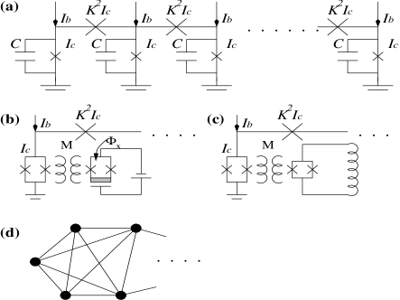
Figure 1: (a) A simple Josephson junction array consisting of $N$ vertical and $N-1$ horizontal junctions. (b) A charge qubit coupled to a vertical junction (realized with a small self-inductance dc-SQUID) in the Josephson junction array in (a). (c) An rf-SQUID qubit coupled to the Josephson junction array. (d) A more complex design than the simple array in (a). Each dot represents a superconducting island which is grounded by a Josephson junction (grounding junctions not shown). Each and every pair of islands are coupled by a Josephson junction as indicated by the edges connecting the dots.

The potential energy of the Josephson junction array in Fig. 1 is a sum of the Josephson tunneling energies of the junctions, given by

$$V=-E_{J}\sum_{i=0}^{N-1}(i_{b}\theta_{i}+\cos{\theta_{i}})-K^{2}E_{J}\sum_{i=0}^{N-2}\cos{(\theta_{i}-\theta_{i+1})},$$

where $E_{J}=I_{c}\Phi_{0}/2\pi$ and $i_{b}=I_{b}/I_{c}$. The equilibrium values for the junction phases are determined by $\partial V/\partial\theta_{i}=0$, which is just the current conservation condition at each node: $i_{b}-\sin{\theta_{i}}-\sin{(\theta_{i}-\theta_{i-1})}-\sin{(\theta_{i}-\theta_{i+1})}=0$. (When $i=0$ or $N-1$ there is only one horizontal current.) In our setup, the equilibrium values for the phases are $\theta_{i}^{(0)}=\theta^{(0)}=\arcsin{i_{b}}$ for $i=0,1,...N-1$. If we are interested in the small oscillations of the phases, we follow the standard procedure expanding $V$ to second order, $V=\frac{1}{2}\sum_{i,j=0}^{N-1}V_{ij}\varphi_{i}\varphi_{j}$, where $\varphi_{i}=\theta_{i}-\theta_{i}^{(0)}$ is the small displacement of the phase from its equilibrium value and

$$\frac{(V)_{ij}}{E_{J}K^{2}}=\delta_{ij}(2+\cos{\theta^{(0)}}/K^{2}-\delta_{i,0}-\delta_{i,N-1})-\delta_{i,j-1}-\delta_{i,j+1}.$$

Notice that the horizontal junctions are much larger than the vertical ones. In the “wash board” analogy this corresponds to a large “mass” for the horizontal junctions. Therefore in calculating the kinetic energy of the system we need only consider the vertical junctions (as verified by numerical calculations): $T=(1/2)C(\Phi_{0}/2\pi)^{2}\sum_{i=0}^{N-1}\dot{\varphi}_{i}^{2}$. From the potential and kinetic energies we can solve for the normal modes of the system, whose spectrum is given by $\nu_{s}=\omega_{p}\sqrt{1+(4K^{2}/\cos{\theta^{(0)}})\sin^{2}(s\pi/2N)}$, where the plasma frequency $\omega_{p}=\sqrt{2\pi I_{c}/\Phi_{0}C}(1-i_{b}^{2})^{1/4}$ and $s=0,1,...,N-1$. Let the orthonormalized normal mode eigenvectors be denoted $b_{i}^{s}$. The lowest mode, whose frequency is $\omega_{p}$, corresponds to the center of mass motion of the phases: $b^{0}=(1,1,...,1)/\sqrt{N}$. The quantum mechanical properties of the small collective vibrational modes of the phases can now be evaluated by introducing the operator $\hat{\varphi_{i}}=(2\pi/\Phi_{0})\sum_{s=0}^{N-1}\sqrt{\hbar/2C\nu_{s}}b_{i}^{s}(a_{s}+a_{s}^{\dagger})$, where $a_{s}$ is the annihilation operator for the $s$th mode.

We propose to use the center of mass motion mode of the Josephson junction array to couple superconducting qubits, in analogy to ion trap quantum computer [23]. Since the center of mass motion mode is an equal weight superposition of the junction phases, its quality factor is as high as that of the individual junctions. Therefore, this approach allows us to take advantage of the high quality Josephson junctions required for the superconducting qubits to realize a high quality resonator. Note in the above we have assumed that all Josephson junctions in the array are identical. In reality, this will not be the case due to unavoidable fabrication errors. However the critical currents of the junctions can be tuned by a magnetic field so that the effective Josephson energies of the junctions can be equalized. The effect of any residual asymmetry can be estimated by perturbation theory. As long as the amplitude of the transition matrix element due to the asymmetry is much smaller than the energy gap between the center of mass motion mode and higher modes, the energy and wavefunction of the center of mass motion mode remain close to unperturbed.

In order to implement protocols developed in superconducting qubit based cavity-QED [13, 14, 15, 16], we need to couple the superconducting qubits to the center of mass motion mode of the junction array in a way such that they can exchange energy. This is shown in Fig. 1 (b) and (c) for both charge and flux qubits. Here each vertical junction in the junction array is replaced by a small self-inductance dc-SQUID and coupled inductively to a superconducting qubit. Consider the charge qubit whose Hamiltonian is $H_{Q}=-B^{z}\sigma^{z}/2-B^{x}\sigma^{x}/2$, where $B^{z}$ and $B^{x}$ are determined by the gate voltage and Josephson energy of the charge qubit. When its energy $B^{z}$ is tuned close to $\nu_{0}=\omega_{p}$ and its dc-SQUID is biased at $\Phi_{0}/2$ (including the flux due to the junction array’s bias current $I_{b}$), the inductive coupling results in a coupling Hamiltonian $H_{c}=-g(a\sigma^{+}+a^{\dagger}\sigma^{-})$, where $g=(M/2)(I_{c}\cos{\theta^{(0)}})I_{c}^{Q}(2\pi/\Phi_{0})\sqrt{\hbar/2C\omega_{p}N}$, $M$ is the mutual inductance, $I_{c}^{Q}$ is the critical current of the dc-SQUID junctions of the charge qubit, and $a$ is the annihilation operator for the center of mass motion mode of the junction array. In deriving $H_{c}$, we have used the rotating wave approximation to drop terms that oscillate at high frequencies. For the flux qubit case shown in Fig. 1 (b), we can derive the same coupling Hamiltonian, with a coupling coefficient which is proportional to the mutual inductance and can be evaluated in terms of the qubit parameters [24]. With the above design we then have a structure in close analogy to the ion trap quantum computer in which the qubits communicate through the center of mass phonon mode. To realize a universal quantum computer, we can use either the resonant [13, 14] or dispersive [13, 15, 16] interaction between the qubits and the junction array mode. The interaction is switched on and off by tuning the energy of the qubit into and out of resonance with the junction array.

Typical values for $\omega_{p}$ and qubit energies can be chosen to be up to 10GHz. The coupling strength $g$ can be tens of megahertz [15, 25]. When the system scales up ($N$ increases), the energy gap between the center of mass motion mode and the higher modes should remain much greater than the coupling strength $g$ to avoid excitation of upper modes. When $N$ is large, the energy difference between the lowest two modes is $\Delta\nu_{01}=(\pi^{2}K^{2}/2N^{2}\cos{\theta^{(0)}})\omega_{p}$. For $K=20$ [26] and $i_{b}=0.97$, this implies an upper limit of a few hundred for $N$. To relax this limit, we can use more complicated designs than the simple 1d array in Fig. 1 (a). For instance, we can consider a network of $N$ superconducting islands in which each pair of nodes is coupled by a Josephson junction, as shown in Fig. 1 (d). Each island is still grounded though a junction whose plasma frequency is $\omega_{p}$, and the Josephson energy of the coupling junctions is $K^{2}$ that of the grounding junctions. In this case, the center of mass motion mode remains at $\omega_{p}$ and all higher modes are pushed up to a frequency $\omega_{p}\sqrt{1+NK^{2}/\cos{\theta^{(0)}}}$. The number of junctions required is on the order $N^{2}/2$.

In the above, we take advantage of the macroscopic quantum behavior of the Josephson junction phases to construct an analogy of the ion trap quantum computer. We can push this concept further and consider using Josephson junction arrays to simulate the dynamics of physical systems. Consider a 1d array of qubits. In the spin 1/2 representation, the dynamics of the qubits are described by the spin operators $S_{i}^{x}$, $S_{i}^{y}$ and $S_{i}^{z}$ whose commutation relations are defined by $[S_{i}^{\alpha},S_{j}^{\beta}]=(i/2)\delta_{ij}\epsilon_{\alpha\beta\gamma}S_{i}^{\gamma}$ for $\alpha,\beta,\gamma=x,y,z$ and $i,j=0,1,...,N-1$. By using a Jordan-Wigner transformation [27], we can map this qubit array to a collection of spinless fermions annihilated by the operators

$$f_{n}=S_{n}^{-}K(n),$$ (1)

where $S_{n}^{\pm}=S_{n}^{x}\pm iS_{n}^{y}$ and $K(n)$ is a nonlocal operator defined by $K(n)=exp[i\pi\sum_{m=0}^{n-1}f_{m}^{+}f_{m}]=exp[i\pi\sum_{m=0}^{n-1}(S_{m}^{z}+1/2)]$. It can be verified that $f_{n}$’s satisfy the anti-commutation relations required for fermion operators. The fermion number operator is simply $f_{n}^{\dagger}f_{n}=S_{n}^{z}+1/2$. Now, if we couple the qubits by nearest neighbor XXZ interactions, the Hamiltonian of the system is $H=-J_{xy}\sum_{i}(S_{i}^{x}S_{i+1}^{x}+S_{i}^{y}S_{i+1}^{y})+J_{z}\sum_{i}S_{i}^{z}S_{i+1}^{z}$. Under the Jordan-Wigner transformation, the system Hamiltonian is transformed to

$$H=-(J_{xy}/2)\sum_{n}(f_{n}^{\dagger}f_{n+1}+f_{n+1}^{\dagger}f_{n})+J_{z}\sum_{n}(f_{n}^{\dagger}f_{n}-1/2)(f_{n+1}^{\dagger}f_{n+1}-1/2).$$ (2)

As can be seen the coupling in the XY directions transforms into hoping of the fermions between neighboring sites and the Ising coupling causes nearest neighbor interactions between the fermions.

Figure 2: A 1d rf-SQUID qubit array inductively coupled to local Josephson junction oscillators. The dc-SQUIDs of the qubits are inductively coupled too. Both $M$ and $M^{\prime}$ are tunable couplings [24, 28, 29]. The qubits are arranged in a ring structure when periodic boundary conditions are required.

An interesting scenario arises when we couple a superconducting qubit array and “phonon modes” realized by small oscillations of Josephson junction phases, as shown in Fig. 2. Since the qubit array can be transformed into a fermion system, this allows us to simulate a family of solid state problems concerning spinless electron-phonon and electron-electron interactions. The macroscopic nature of the system and the fine control and measurement techniques developed in superconducting quantum information processing allow us to examine the fermion dynamics directly and closely to obtain vital information about the system. For this purpose, we need to be careful with a few issues. The first is that in a physical system the electron number is conserved; however a $B^{x}\sigma^{x}$ term of the qubit can flip its basis states defined by the eigenstates of $\sigma^{z}$. According to the Jordan-Wigner transformation Eq. (1) the flipping of the qubit state corresponds to the creation or annihilation of a fermion. Therefore, we must keep $B^{x}$ of the qubits zero. This is realized by using small self-inductance dc-SQUIDs for the qubits and biasing them appropriately so that the $B^{x}$ field of the qubit is much smaller [15] than other energy scales of the system and thus can be neglected for the time scale of interest. To further suppress fermion creation and annihilation, we may choose $B^{z}$ to be large, which makes changes in the total number of fermions energetically forbidden. Another point is that the coupling between the qubit and the Josephson phase should not allow them to exchange excitations, since in a physical system no process happens in which an electron is created (annihilated) and a phonon is annihilated (created).

In the following we focus on the 1d Holstein model of spinless electrons, a problem of both theoretical and practical interest [30, 31]. The Hamiltonian of the system is

$$H=-t\sum_{i}(c_{i}^{\dagger}c_{i+1}+c_{i+1}^{\dagger}c_{i})+\omega\sum_{i}a_{i}^{\dagger}a_{i}-g\sum_{i}(c_{i}^{\dagger}c_{i}-1/2)(a_{i}+a_{i}^{\dagger}),$$ (3)

where $c_{i}$ destroys a fermion at site $i$ and $a_{i}$ destroys a local phonon of frequency $\omega$. This system at half filling has two phases depending on the ratio $g/\omega$. When $g<g_{c}$, the ground state has a metallic (Luttinger liquid) phase. When $g$ exceeds $g_{c}$, it exhibits an insulating phase with charge density wave (CDW) long range order [30, 31]. Though it can be solved analytically in certain limits, for generic parameters the accurate determination of the critical coupling strength and energy gaps is difficult and only limited size systems at half filling have been studied numerically [30, 31].

We can construct an artificial realization of the 1d Holstein model using a superconducting qubit array and local oscillator modes realized by Josephson junctions, as shown in Fig. 2. For clarity, rf-SQUID qubits are shown, whose dc-SQUIDs are coupled by a tunable mutual inductance. The tunable mutual inductances can be realized by using a flux transformer interrupted by a dc-SQUID whose critical current can be tuned by a flux bias, as discussed in [24, 28, 29]. As a result of this inter-qubit coupling and the qubit bias, the qubit array Hamiltonian is $H_{Q}=-\sum_{i}B^{z}S_{i}^{z}-J\sum_{i}S_{i}^{x}S_{i+1}^{x}$, where $B^{z}$ is determined by the flux bias of the qubits and $J$ is proportional to the tunable mutual inductance $M$. The local phonon modes are realized by Josephson junctions whose oscillation frequency is the plasma frequency $\omega_{p}$. These junctions should have a deep potential well in order to guarantee that their behavior is close to harmonic even when the excitation number is not small. Alternatively, if we are also interested in studying the effect of nonharmonicity of the phonon modes on the system behavior [32], we may use an inductor ($L$) shunted dc-SQUID. In this case, under the condition $LI_{c}\ll\Phi_{0}/2\pi$, the Hamiltonian for the phonon mode is $Q^{2}/2C_{J}+\Phi^{2}/2L^{\prime}-(I_{c}/24)(2\pi/\Phi_{0})^{3}\Phi^{4}$, where $Q$ and $\Phi$ are the charge and flux across the dc-SQUID, $C_{J}$ is the total junction capacitance and the effective inductance $L^{\prime}=L(1-2\pi LI_{c}/\Phi_{0})$. The anharmonicity can be adjusted by tuning the critical current $I_{c}$ of the dc-SQUID.

The local Josephson junction oscillators are coupled to the main loops of the rf-SQUID qubits using a tunable mutual inductance as shown in Fig. 2. This introduces a coupling Hamiltonian proportional to $S^{z}\Phi$, with a coupling coefficient proportional to the mutual inductance $M^{\prime}$[24]. After quantizing the local phonon modes and applying the Jordan-Wigner transformation, we obtain the Hamiltonian of the 1d Holstein model Eq. (3), with the hopping strength $t=J/4$ and the phonon frequency $\omega=\omega_{p}$. Since the qubit-qubit and qubit-phonon interactions are realized with tunable couplings, the ratio of $t$ and $g$ to $\omega$ in the Holstein model can be tuned in a wide range. This allows us to explore a large phase space of the system. To simulate the 1d Holstein model, we first set the number of spinless fermions in the system. This is done by initializing half the qubits in the $S^{z}=1/2$ state and the other half in the $S^{z}=-1/2$ state (assuming we are interested in the half filling case), which can be accomplished by applying strong $B^{z}$ fields to the qubits or by performing measurements. Then $t$ and $g$ are turned on (by tuning the inter-qubit and qubit phonon couplings) slowly until the intended point $(t,g,\omega)$ in the phase space is reached. The phase of the system can be inferred by measuring the fermion numbers $f_{n}^{\dagger}f_{n}$, or $S_{n}^{z}$, which are independent of $n$ (1/2 for half filling) for the metallic phase and varying with $n$ for the insulating phase. The excitation energy of the system can be determined by spectroscopic methods like in [18].

In conclusion, we have shown that properly engineered Josephson junction arrays can be used for quantum manipulation and simulation. The discussed protocols require only limited control of the system and provide interesting opportunities for superconducting quantum information processing.

The authors acknowledge financial support from the Packard Foundation.

References

- [1] Y. Makhlin, G. Schön, and A. Shnirman, Rev. Mod. Phys. 73, 357 (2001).
- [2] Y. Nakamura, Y. A. Pashkin, and J. S. Tsai, Nature (London) 398, 786 (1999).
- [3] J. R. Friedman, V. Patel, W. Chen, S. K. Tolpygo, and J. E. Lukens, Nature 406, 43 (2000).
- [4] C. H. van der Wal, A. C. J. ter Haar, F. K. Wilhelm, R. N. Schouten, C. J. P. M. Harmans, T. P. Orlando, S. Lloyd, and J. E. Mooij, Science 290, 773 (2000).
- [5] D. Vion, A. Aassime, A. Cottet, P. Joyez, H. Pothier, C. Urbina, D. Esteve, and M. H. Devoret, Science 296, 886 (2002).
- [6] Y. Yu, S. Han, X. Chu, S-I.Chu, and Z. Wang, Science 296, 889 (2002).
- [7] J. M. Martinis S. Nam, J. Aumentado, and C. Urbina, Phys. Rev. Lett. 89, 117901 (2002).
- [8] I. Chiorescu, Y. Nakamura, C. J. P. M. Harmans, and J. E. Mooij, Science 299, 1869 (2003).
- [9] Y. A. Pashkin, T. Yamamoto, O. Astafiev, Y. Nakamura, D. V. Averin, and J. S. Tsai, Nature (London) 421, 823 (2003); T. Yamamoto, Yu. A. Pashkin, O. Astafiev, Y. Nakamura, and J. S. Tsai, ibid., 425, 941 (2003).
- [10] A. J. Berkley, H. Xu, R. C. Ramos, M. A. Gubrud, F. W. Strauch, P. R. Johnson, J. R. Anderson, A. J. Dragt, C. J. Lobb, and F. C. Wellstood, Science 300, 1548 (2003).
- [11] A. Izmalkov, M. Grajcar, E. Il’ichev, Th. Wagner, H.-G. Meyer, A. Yu. Smirnov, M. H. S. Amin, A. M. van den Brink, and A. M. Zagoskin, Phys. Rev. Lett. 93, 037003 (2004).
- [12] I. Chiorescu, P. Bertet, K. Semba, Y. Nakamura, C. J. P. M. Harmans, and J. E. Mooij, Nature (London) 431, 159 (2004).
- [13] F. Plastina and G. Falci, Phys. Rev. B 67, 224514 (2003).
- [14] A. Blais, A. M. van den Brink, and A. M. Zagoskin, Phys. Rev. Lett. 90, 127901 (2003).
- [15] X. Zhou, M. Wulf, Z-W. Zhou, G-C. Guo, and M. J. Feldman, Phys. Rev. A 69, 030301R (2004).
- [16] A. Blais, R-S. Huang, A. Wallraff, S. M. Girvin, and R. J. Schoelkopf, Phys. Rev. A 69, 062320 (2004).
- [17] A. Wallraff, D. I. Schuster, A. Blais, L. Frunzio, R-S. Huang, J. Majer, S. Kumar, S. M. Girvin, and R. J. Schoelkopf, Nature (London) 431, 162 (2004).
- [18] H. Xu, F. W. Strauch, S. Dutta, P. R. Johnson, R. C. Ramos, A. J. Berkley, H. Paik, J. R. Anderson, A. J. Dragt, C. J. Lobb, and F. C. Wellstood, Phys. Rev. Lett. 94, 027003 (2005).
- [19] A. M. Kadin, “Introduction to superconducting circuits,” Wiley-Interscience, 1999.
- [20] B. A. Mazin, P. K. Day, H. G. LeDuc, A. Vayonakis, and J. Zmuidzinas, Proc. SPIE 4849, 283 (2002).
- [21] P. K. Day, H. G. Leduc, B. A. Mazin, A. Vayonakis, and J. Zmuidzinas, Nature 425, 817 (2003).
- [22] N. Rando, P. Videler, A. Peacock, A. van Dordrecht, P. Verhoeve, R. Venn, A. C. Wright, and J. Lumley, J. Appl. Phys. 77, 4099 (1995).
- [23] J. I. Cirac and P. Zoller, Phys. Rev. Lett. 74, 4091 (1995).
- [24] T. P. Orlando, J. E. Mooij, L. Tian, C. H. van der Wal, L. S. Levitov, S. Lloyd, and J. J. Mazo, Phys. Rev. B. 60, 15398 (1999).
- [25] J. Q. You, C-H. Lam, and H. Z. Zheng, Phys. Rev. B 63, 180501R (2001). J. Q. You, J. S. Tsai, and F. Nori, Phys. Rev. Lett. 89, 197902 (2002).
- [26] Notice as mentioned earlier is not necessarily the ratio of junction sizes since magnetic suppression of critical currents is usually needed.
- [27] P. Jordan and E. Wigner, Z. Phys. 47, 631 (1928).
- [28] J. E. Mooij, T. P. Orlando, L. Levitov, L. Tian, C. H. van der Wal, and S.Lloyd, Science 285, 1036 (1999).
- [29] T. V. Filippov, S. K. Tolpygo, J. Mannik, and J. E. Lukens, IEEE Trans. Appl. Supercond. 13, 1005 (2003).
- [30] R. H. McKenzie, C. J. Hamer, and D. W. Murray, Phys. Rev. B. 53, 9676 (1996).
- [31] R. J. Bursill, R. H. McKenzie, and C. J. Hamer, Phys. Rev. Lett. 80, 5607 (1998).
- [32] J. K. Freericks, M. Jarrell, and G. D. Mahan, Phys. Rev. Lett. 77, 4588 (1996).