Nonlinear coupling of nano mechanical resonators to Josephson quantum circuits

Abstract

We propose a technique to couple the position operator of a nano mechanical resonator to a SQUID device by modulating its magnetic flux bias. By tuning the magnetic field properly, either linear or quadratic couplings can be realized, with a discretely adjustable coupling strength. This provides a way to realize coherent nonlinear effects in a nano mechanical resonator by coupling it to a Josephson quantum circuit. As an example, we show how squeezing of the nano mechanical resonator state can be realized with this technique. We also propose a simple method to measure the uncertainty in the position of the nano mechanical resonator without quantum state tomography.

Introduction. Historically, mechanical systems have not been the favorite proving ground of quantum mechanics because of their macroscopic nature. This situation has changed in recent years thanks to the impressive advance of nano fabrication technologies. It is now possible to make nano mechanical resonators with frequencies of gigahertz ref:Huang03 and quality factors approaching $10^{5}$ at milli Kelvin temperatures ref:NEMS . This opens the possibility of studying coherent quantum behavior in mesoscopic mechanical systems ref:Armour02 ; ref:Tian04 . One can also exploit the quantum properties of mechanical degrees of freedom for applications in areas such as weak force detection ref:Bocko96 , precision measurement ref:Munro02 , and quantum information processing ref:Cleland04 . Recently, evidence for quantized displacement in a nano mechanical resonator has been observed ref:Gaidarzhy05 .

All micro and nano mechanical devices require some means of transduction. As discussed in ref:Armour02 , an excellent way to engineer and detect the quantum modes of a nano mechanical resonator is to couple the resonator to Josephson device based solid state circuitry ref:Makhlin01 on which quantum coherent control has been demonstrated. A straightforward coupling scheme for this purpose is to voltage bias the resonator and use the position dependent electrostatic interaction between the nano resonator and a charge island. This is discussed in ref:Armour02 and used in all previous studies (see ref:Armour02_cited for an incomplete list). Though conceptually simple and practically feasible, this scheme has the limitation that the dominant term in the induced coupling is always linear in the resonator position. Consequently, it can only be used to realize linear effects in the nano resonator. As is well known in quantum optics ref:QO , nonlinear effects are indispensable for thorough study and control of the dynamics of harmonic oscillators. They are required to produce essential processes such as squeezing and parametric amplification. They are also known to be necessary for universal quantum information processing on continuous variables ref:Braunstein05 . Thus, it is highly desirable to develop new coupling schemes which can introduce nonlinear effects into the nano resonator system.

In this work, we propose an attractive alternative method to couple the nano mechanical resonator to a Josephson quantum circuit by modulating the flux bias of a SQUID device. Our scheme makes it possible to realize both linear and nonlinear processes on the nano mechanical resonator. We show how we can generate squeezing of the nano mechanical resonator using this method and propose a simple way to measure the reduction in the uncertainty in the resonator’s position.

The device and its working principle. Our scheme is illustrated in Fig. 1 (a). Here, the nano mechanical resonator is in one arm of a SQUID device. The SQUID loop is biased with a perpendicular magnetic field $B$, such that the flux threading the SQUID is the product of $B$ and the area of the SQUID loop.

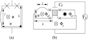
Figure 1: (a) A nano mechanical resonator in one arm of a SQUID device. The SQUID loop is threaded by a magnetic field. Its flux bias will then depend on the position of the nano mechanical resonator. (b) A more complicated design in which a nano mechanical resonator is coupled to a charge qubit. The shaded box is the superconducting island of the charge qubit.

We see that the area of the SQUID loop is dependent on the position of the nano mechanical resonator. In Fig. 1 (a), we denote the width and length of the SQUID loop $W$ and $L$. The length and small displacement of the nano mechanical resonator are $l$ and $X$, defined such that the area of the SQUID loop is $WL+lX$. The total flux bias of the SQUID loop is $\Phi_{e}^{0}+BlX$, where $\Phi_{e}^{0}=BWL$ is the flux bias corresponding to the equilibrium position of the nano mechanical resonator. With the phase drops of the two junctions being $\phi_{1}$ and $\phi_{2}$, the Josephson energy of the SQUID is $E_{J}=-E_{J}^{0}\cos\phi_{1}-E_{J}^{0}\cos\phi_{2}=-2E_{J}^{0}\cos(\phi_{1}-\phi_{2})/2\cos(\phi_{1}+\phi_{2})$, where $E_{J}^{0}=I_{c}\Phi_{0}/2\pi$ is the Josephson energy of the (identical) junctions, $I_{c}$ the junction critical current and $\Phi_{0}$ the flux quantum. Since the superconducting order parameter is singly valued, we must have $\phi_{1}-\phi_{2}+2\pi(\Phi_{e}^{0}+BlX)/\Phi_{0}=2\pi p$ for some integer $p$ leading to ref:E_J_note

$$E_{J}=-2E_{J}^{0}\cos(\frac{\pi\Phi_{e}^{0}}{\Phi_{0}}+\frac{\pi Bl}{\Phi_{0}}X)\cos\phi,$$ (1)

where $\phi=(\phi_{1}+\phi_{2})/2$ is the average phase across the junctions.

It is clear from Eq. (1) that in general the Josephson energy of the SQUID is a nonlinear function of $X$, the position of the nano mechanical resonator. Treating $X$ as a small perturbation, we find that there are two flux bias points of particular interest: $\Phi_{e}^{0}=(n+1/2)\Phi_{0}$ and $\Phi_{e}^{0}=n\Phi_{0}$, where $n$ is an integer. When $\Phi_{e}^{0}=(n+1/2)\Phi_{0}$, to lowest order in $X$ the Josephson energy of the SQUID is $E_{J}=(-1)^{n}2E_{J}^{0}(\pi(n+1/2)l/WL)X\cos\phi$. In this case, $E_{J}$ has a linear dependence on $X$ and thus linear coupling between the nano resonator and SQUID is realized. On the other hand, when the SQUID loop is biased at $\Phi_{e}^{0}=n\Phi_{0}$, to lowest order in $X$ the Josephson energy is

$$E_{J}=-(-1)^{n}2E_{J}^{0}\{1-(\pi nl/WL)^{2}X^{2}/2\}\cos\phi.$$ (2)

Here, the Josephson energy of the SQUID has a quadratic dependence on the position of the nano mechanical resonator.

From the perspective of micro and nano mechanical engineering, our coupling scheme can be considered a magnetic transduction method. Compared to the electrostatic transduction scheme ref:Armour02 , the distinctive advantage of our scheme is that the coupling can be either linear or quadratic, depending on the flux bias point of the SQUID. Also, notice that the coupling strength can be adjusted (discretely), since $E_{J}$ depends on $n$ as in Eq. (2). It is then possible in principle to operate in both linear and nonlinear, as well as both weak and strong, coupling regimes. In practice, the SQUID will be part of a Josephson quantum circuit (for instance a charge or flux qubit), and the modulation scheme above then couples the nano mechanical oscillator to the Josephson quantum circuit.

Note the nano mechanical resonator must be superconducting for our scheme to work. This can be realized by using a metalized resonator ref:NEMS ; ref:Schwab02 as long as the magnetic field does not exceed the critical field strength of the superconductor.

Squeezing of the nano mechanical resonator. An important nonlinear effect on a harmonic oscillator is squeezing. It is the suppression of the uncertainty in the position (or momentum) of the oscillator at the price of increased uncertainty in the conjugate variable. For nano mechanical resonators, reduction in the position uncertainty is important in applications such as weak force detection ref:Bocko96 . Also, some coherent nonlinear process such as squeezing is essential for universal quantum information processing on continuous variables ref:Braunstein05 . Our nonlinear coupling scheme makes such coherent nonlinear processes inaccessible by previous methods ref:Armour02 ; ref:Armour02_cited possible. This provides a way of introducing nonlinear-effect-induced operators, for instance, as gates within a complicated quantum circuit. Previously, generation of certain squeezed states of nano mechanical resonators has been studied by a few authors ref:Rabl04 ; ref:Ruskov05 . However, since no coherent nonlinear transduction scheme on the nano mechanical resonator was known, these schemes had to function incoherently. They used dissipation and measurement to generate the needed nonlinearity and were incapable of effecting unitary evolutions.

In the following we show how we can realize squeezing on a nano mechanical resonator using our scheme to couple it to a charge qubit ref:Shnirman97 . First, we notice that the simple prototype circuit in Fig. 1 (a), though convenient in illustrating the essence of our scheme, has a few disadvantages. In particular, according to Eq. (2), when a nonlinear coupling is realized the Josephson self-energy is also the largest ($2E_{J}^{0}$), therefore we do not have completely independent control over the coupling strength and Josephson self-energy. To overcome this and other disadvantages, we consider the design shown in Fig. 1 (b). Here, we have two identical SQUIDs (left and right) biased at equal but opposite fluxes $\Phi_{el}=-\Phi_{er}=BWL$ (this can be realized by twisting the arms of one of the SQUIDs, for instance). The nano mechanical resonator is in the arm of one of the SQUIDs and coupled to its phase. The big loop is biased with an external flux $\Phi_{x}$. This structure bears some similarity to the scalable charge qubit scheme in ref:You02 , and the advantage is that both the flux biases of the individual SQUIDs and the big loop can be tuned.

In order to realize nonlinear coupling between the nano mechanical resonator and the charge qubit, we bias the SQUIDs at $\Phi_{el}=-\Phi_{er}=n\Phi_{0}$. Using the same argument that leads to Eq. (2), we can derive the Josephson energy of the circuit in Fig. 1 (b). To lowest order in the resonator position $X$, $E_{J}=-(-1)^{n}4E_{J}^{0}\cos(\pi\Phi_{x}/\Phi_{0})\cos\phi+(-1)^{n}E_{J}^{0}(\pi nl/WL)^{2}X^{2}\cos\phi_{l}$, where $\phi_{l}$ and $\phi_{r}$ are the phases of the left and right SQUIDs (the averages of the phases of the two junctions in the SQUIDs), and $\phi=(\phi_{l}+\phi_{r})/2$ is the average phase of the SQUIDs conjugate to the charge number on the island. If we bias the big loop at $\Phi_{x}=(2m+1/2)\Phi_{0}$, $m$ an integer, only the coupling term survives, so $E_{J}=(-1)^{n}E_{J}^{0}(\pi nl/WL)^{2}X^{2}\cos\phi_{l}$.

The charge island possesses an adjustable gate voltage $V_{g}$ which is applied through the gate capacitance $C_{g}$. When it is biased close to $n_{g}=C_{g}V_{g}/2e=1/2$, the states with $0$ and $1$ excess Cooper pairs comprise the low energy Hilbert space of the qubit. Considering these charge states the spin up and spin down states ref:Armour02 in an effective two state system, we can use the Pauli matrices to describe operators acting on the system, and its uncoupled Hamiltonian takes the form $E_{z}\sigma_{z}/2$, where $E_{z}=(2n_{g}-1)(2e)^{2}/2C_{t}$ and $C_{t}$ is the total capacitance of the charge island.

As usual, the nano resonator is treated as a harmonic oscillator with position operator $X=\delta X_{0}(a+a^{\dagger})$ ref:Armour02 , where $a$ is the annihilation operator, $\delta X_{0}=\sqrt{\hbar/2M\omega_{0}}$ is the zero point fluctuation in the resonator’s position $X$, and $M$ and $\omega_{0}$ are the mass and frequency of the resonator. Its uncoupled Hamiltonian is $\omega_{0}a^{\dagger}a$.

The system Hamiltonian is then $H=E_{z}\sigma_{z}/2+\omega_{0}a^{\dagger}a-(\lambda_{n}/2)(a+a^{\dagger})^{2}\sigma_{y}$, where the coupling strength $\lambda_{n}=-(-1)^{n}E_{J}^{0}(\pi nl\delta X_{0}/WL)^{2}$. If we choose $E_{z}=2\omega_{0}$ and shift to the rotating frame defined by $E_{z}\sigma_{z}/2+\omega_{0}a^{\dagger}a$, we obtain the following Hamiltonian in the rotating frame ref:QO :

$$H_{R}=i(\lambda_{n}/2)(a^{2}\sigma^{+}-a^{\dagger 2}\sigma^{-})+H_{\omega_{0}},$$ (3)

where $\sigma^{\pm}=(\sigma_{x}\pm i\sigma_{y})/2$ and $H_{\omega_{0}}$ are off resonance terms of magnitude $\lambda_{n}/2$ oscillating at frequencies of $2\omega_{0}$ and higher. Since the realizable coupling strength $\lambda_{n}$ is usually much smaller than the resonator frequency $\omega_{0}$, we can adopt the rotating wave approximation to drop $H_{\omega_{0}}$ ref:QO .

In addition to the operating point discussed above, we also consider another set of bias conditions in which the SQUIDs are biased at 0 flux and $E_{z}$ is changed (by tuning the gate voltage $V_{g}$) to $E_{z}^{\prime}=2\omega_{0}+\delta E_{z}$. We also bias the big loop slightly away from $(2m+1/2)\Phi_{0}$ using a small ac field, $\Phi_{x}=(2m+1/2)\Phi_{0}+\delta\Phi_{x}\cos 2\omega_{0}t$ where $\pi\delta\Phi_{x}/\Phi_{0}\ll 1$. In this case the charge qubit is decoupled from the resonator. To lowest order in $\pi\delta\Phi_{x}/\Phi_{0}$, the system Hamiltonian in the same rotating frame is $H=\delta E_{z}\sigma_{z}/2+E_{x}\sigma_{x}/2+H^{\prime}_{\omega_{0}}$, where $E_{x}=4E_{J}^{0}(\pi\delta\Phi_{x}/\Phi_{0})$ and the rapidly oscillating term $H^{\prime}_{\omega_{0}}$ will have negligible effect if $E_{x}$ is small compared to $4\omega_{0}$ and the system evolves for an appropriate duration ref:Wei63 . In the above Hamiltonian both $\delta E_{z}$ and $E_{x}$ of the qubit can be adjusted ref:Armour02 ; therefore we can perform arbitrary rotations on the state of the charge qubit. In particular, if we choose large values for $\delta E_{z}$ and $E_{x}$, we can realize pulsed operations on the charge qubit and flip its state quickly.

We now consider a spin echo like process in which we let the system evolve under the Hamiltonian (3) for short periods of time of duration $\Delta t$. In between each such time interval we apply a quick $\pi$ pulse $\sigma_{x}$ to the charge qubit to flip its state, so that the evolution for two periods is governed by $\exp\{-iH_{R}\Delta t\}\sigma_{x}\exp\{-iH_{R}\Delta t\}\sigma_{x}$. Since $\sigma_{x}\exp\{(\lambda_{n}\Delta t/4)[(a^{2}-a^{\dagger 2})\sigma_{x}+i(a^{2}+a^{\dagger 2})\sigma_{y}]\}\sigma_{x}$ $=\exp\{(\lambda_{n}\Delta t/4)[(a^{2}-a^{\dagger 2})\sigma_{x}-i(a^{2}+a^{\dagger 2})\sigma_{y}]\}$, this evolution operator can be simplified: $\exp\{-iH_{R}\Delta t\}\sigma_{x}\exp\{-iH_{R}\Delta t\}\sigma_{x}\approx\exp\{(\lambda_{n}\Delta t/2)(a^{2}-a^{\dagger 2})\sigma_{x}\}$. If we initialize the charge qubit in the $\sigma_{x}=1$ state, and repeat this procedure $N$ times, the evolution operator on the state of the resonator becomes

$$S(\kappa)=\exp\{\frac{\kappa}{2}(a^{2}-a^{\dagger 2})\},$$ (4)

where $\kappa=\lambda_{n}N\Delta t$. This is a squeezing operator on the nano mechanical resonator with squeezing parameter $\kappa$. Under the squeezing operator, $a$ transforms to $S^{\dagger}(\kappa)aS(\kappa)=a\cosh\kappa-a^{\dagger}\sinh(\kappa)$ and it can be shown that the position uncertainty decreases exponentially ref:QO : $\Delta X=\sqrt{\langle X^{2}\rangle-\langle X\rangle^{2}}=\Delta X(0)e^{-\kappa}$.

In the above, we used a multi-loop circuit which allows bias and control of the individual loops. Such structure and control are easy to realize and widely used in current Josephson quantum circuit design and experiment ref:You02 ; ref:Mooij99 ; ref:Mooij03 . Also, high-precision spin echo control of superconducting qubits has been realized experimentally ref:ChargeEcho . Sophisticated microwave pulse sequences can be applied and it was observed that the decoherence time of the superconducting qubit increases due to the spin echo control. Therefore, our scheme is within the reach of current technologies.

Ideally, one would like a large coupling strength in order to generate appreciable squeezing in a short period of time. For a magnetic field $B\approx 0.2$T, $l\approx 30\mu$m, $\delta X_{0}\approx 5\times 10^{-13}$m, and a critical current of about $60$nA, the coupling strength $\lambda_{n}$ is about $4$MHz.

Decoherence. Unlike previous methods ref:Rabl04 ; ref:Ruskov05 , our scheme effects a coherent quantum process. The influence of decoherence must be considered in detail. For this purpose, we use the Master equation ref:QO

$$d\rho/dt=-i[H_{sq},\rho]+\mathcal{L}(a,\gamma_{n},N_{n})+\mathcal{L}(\sigma^{-},\gamma_{q},N_{q})+\mathcal{L}(\sigma_{z},\gamma_{\phi},N_{q}),$$ (5)

where $\rho$ is the density matrix of the nano resonator - charge qubit system, $H_{sq}=i\lambda(a^{2}-a^{\dagger 2})\sigma_{x}/2$ is the effective squeezing Hamiltonian, $\gamma_{n}=\omega_{0}/Q$ is the decay rate of the nano mechanical resonator determined by its quality factor $Q$, $\gamma_{q}$ and $\gamma_{\phi}$ are the relaxation and dephasing rate of the charge qubit, $N_{n}$ and $N_{q}$ are the mean values of the bath quanta dependent on temperature ref:QO , and the Liouvillian operator $\mathcal{L}(A,\gamma,N)=(1/2)\gamma(N+1)(2A\rho A^{\dagger}-A^{\dagger}A\rho-\rho A^{\dagger}A)+(1/2)\gamma N(2A^{\dagger}\rho A-AA^{\dagger}\rho-\rho AA^{\dagger})$. Among the various decoherence sources, the dephasing of the charge qubit is dominant. For most nano mechanical resonator frequencies ref:NEMS , we only bias the charge qubit slightly away from the charge degeneracy point ($|2n_{g}-1|\ll 0.1$) and the dephasing time $T_{2}$ is greater than $100$ns ref:Moon05 . Using the Master equation we can derive equations for the expectation values of the dynamic variables of the system which are then solved. In Fig. 2 (a), we plot the time dependence of the nano resonator position uncertainty $\Delta X$. We have used the following conservative set of experimental parameters: resonator frequency $\omega_{0}/2\pi=250$MHz, quality factor $Q=10^{4}$, temperature $T=20$mK, squeezing parameter $\lambda=5$MHz, with $\gamma_{q}$ and $\gamma_{\phi}$ chosen such that the relaxation time $T_{1}=1\mu$s and dephasing time $T_{2}=100$ns ref:Moon05 . Initially the nano resonator is assumed to be in a thermal equilibrium state and the charge qubit is in the $\sigma_{x}=1$ state.

It is clear from Fig. 2 (a) that appreciable squeezing can be generated even when the charge qubit’s dephasing rate is severe (twice the squeezing parameter), indicating that the squeezing is robust against decoherence. As time progresses, the squeezing becomes less effective and eventually $\Delta X$ starts to increase. This is easy to understand from the effective Hamiltonian $i\lambda(a^{2}-a^{\dagger 2})\sigma_{x}$ leading to (4); as the charge qubit dephases, $\langle\sigma_{x}\rangle$ decreases and the squeezing effect weakens and eventually disappears. Not surprisingly, the maximum squeezing achievable increases with decreasing dephasing rate, as shown in Fig. 2 (b).

Figure 2: (a) Time dependence of the nano resonator position uncertainty $\Delta X$ (normalized to the initial uncertainty) under the effect of squeezing and decoherence. See text for experimental parameters and initial conditions. (b) The maximum achievable squeezing (minimum $\Delta X$) as a function of the dephasing rate. All other parameters are the same as in (a).

Measurement. Once we generate squeezing on the nano mechanical resonator, a scheme is needed to measure the uncertainty in its position to confirm the squeezing effect. One way to do this is quantum tomography which measures the resonator’s Wigner function. As shown in ref:Lutterbach97 , the Wigner function can be measured by displacing the state of the harmonic oscillator, letting it interact with a two state system, and measuring the polarization of the two state system. Though this method can determine all the information about the oscillator, its direct application in our solid state system is hindered by technical difficulties. To displace the resonator’s state arbitrarily, we will need couplings to both the position and momentum operators of the resonator with continuously variable relative strengths, which is not easy to realize in the nano resonator. Also, in order to calculate $\Delta X$, we need the Wigner function over its entire parameter space making it necessary to sweep through a large parameter space. Large displacement will take a long time to effect and the decoherence will affect the measurement result.

Here we propose a simplified method to measure the mean and variance of the position operator of the nano resonator. It is based on the measurement of the generating function $Tr(\rho e^{i\kappa X})$. We notice that $\langle X\rangle$ and $\langle X^{2}\rangle$ can be calculated from the generating function by

$$\langle X\rangle=Tr(\rho X)=-i\frac{d}{d\kappa}Tr(\rho e^{i\kappa X})|_{\kappa=0}$$ (6)

and

$$\langle X^{2}\rangle=Tr(\rho X^{2})=-\frac{d^{2}}{d\kappa^{2}}Tr(\rho e^{i\kappa X})|_{\kappa=0}.$$ (7)

Therefore, measuring the generating function in the vicinity of $\kappa=0$ allows us to determine the position uncertainty of the nano mechanical resonator $\Delta X^{2}$.

The generating function can be measured by first preparing the charge qubit in the $\sigma_{z}=1$ state. Then turning on a strong coupling $\lambda X\sigma_{x}$ between the charge qubit and the resonator, for a time $t$, will cause the charge qubit states corresponding to $\sigma_{x}=\pm 1$ to acquire a phase shift $\mp\lambda tX$. Next, the interaction is turned off and the gate $\textsf{H}\exp\{i(\pi/4)(\vec{n}\cdot\vec{\sigma})\}$ is applied to the charge qubit, where $\textsf{H}=(\sigma_{x}+\sigma_{z})/\sqrt{2}$ is the Hadamard gate, $\vec{n}=(0,-\cos{\eta},\sin{\eta})$, $\eta$ an angle chosen to be 0 or $\pi/2$. We then measure the polarization of the charge qubit, $\langle\sigma_{z}\rangle=P_{\sigma_{z}=1}-P_{\sigma_{z}=-1}$, which can be shown to equal ref:Lutterbach97

$$Tr(\rho Re\{e^{i\eta}e^{i\kappa X}\}),$$ (8)

where $\kappa=2\lambda t$. Choosing $\eta=0$ and $\pi/2$ then yields the real and imaginary part of the generating function, which in turn allows us to calculate $\Delta X^{2}$ by Eqs. (6) and (7).

This method based on the measurement of the generating function has a few attractive advantages. It requires only strong linear coupling of the charge qubit to the position operator of the resonator, which as discussed before can be easily realized in our scheme by biasing the SQUIDs at $(n+1/2)\Phi_{0}$ and the big loop at 0 flux. We only need to measure in the vicinity of $\kappa=0$, therefore the measurement can be done quickly, implying less influence by decoherence. Since the polarization of the charge qubit can be measured with high fidelity ref:Vion02 , our scheme is realistic given currently available technology.

Conclusion. We have proposed a scheme to couple a nano mechanical resonator to Josephson quantum circuits by modulating the magnetic bias of a SQUID. This allows us to realize coherent nonlinear effects on the nano resonator, which are essential for but so far missing in the study of nano mechanical resonators. Though we focused on the squeezing of a nano mechanical resonator by coupling it to a charge qubit, our scheme can be easily tailored to other purposes and adapted for coupling to other Josephson quantum circuits. It can be directly extended for quantum manipulation of multiple nano resonators. Then, entanglement can be generated and confirmed using the simple measurement scheme. This can provide a practically feasible approach for unambiguous demonstration of quantum behavior in nano mechanical resonators.

The authors acknowledge financial support from the Packard foundation.

References

- (1) X. M. H. Huang, C. A. Zorman, M. Mehregany, and M. L. Roukes, Nature 421, 496 (2003).
- (2) R. G. Knobel and A. N. Cleland, Nature 421, 291 (2003); M. D. LaHaye, O. Buu, B. Camarota, and K. C. Schwab, Science 304, 74 (2004).
- (3) A. D. Armour, M. P. Blencowe, and K. C. Schwab, Phys. Rev. Lett. 88, 148301 (2002).
- (4) L. Tian, Phys. Rev. B 72, 195411 (2005).
- (5) M. F. Bocko and R. Onofrio, Rev. Mod. Phys. 68, 755 (1996).
- (6) W. J. Munro, K. Nemoto, G. J. Milburn, and S. L. Braunstein, Phys. Rev. A 66, 023819 (2002).
- (7) A. N. Cleland and M. R. Geller, Phys. Rev. Lett. 93, 070501 (2004).
- (8) A. Gaidarzhy, G. Zolfagharkhani, R. L. Badzey, and P. Mohanty, Phys. Rev. Lett. 94, 030402 (2005). See also K. C. Schwab et al., quant-ph/0503018 and A. Gaidarzhy et al., cond-mat/0503502.
- (9) Y. Makhlin, G. Schön and A. Shnirman, Rev. Mod. Phys. 73, 357 (2001).
- (10) E. K. Irish and K. Schwab, Phys. Rev. B 68, 155311 (2003). I. Wilson-Rae, P. Zoller, and A. Imamoglu, Phys. Rev. Lett. 92, 075507 (2004). I. Martin et al., Phys. Rev. B 69, 125339 (2004). M. R. Geller and A. N. Cleland, Phys. Rev. A 71, 032311 (2005). P. Zhang et al., Phys. Rev. Lett. 95, 097204.
- (11) M. O. Scully and M. S. Zubairy, Quantum Optics, Cambridge University Press, 1997. D. F. Walls and G. J. Milburn, Quantum Optics, Springer, New York, 1994.
- (12) S. L. Braunstein and P. van Loock, Rev. Mod. Phys. 77, 513 (2005).
- (13) A. M. Kadin, Introduction to superconducting circuits, Wiley, 1999. Here we assume that the self inductance of the SQUID is small and neglect its effect. Including the effect of the self inductance results in more complicated expressions but does not change the conclusion in a qualitative way.
- (14) K. C. Schwab, Appl. Phys. Lett. 80, 1276 (2002).
- (15) P. Rabl, A. Shnirman, and P. Zoller, Phys. Rev. B 70, 205304 (2004).
- (16) R. Ruskov, K. Schwab, and A. N. Korotkov, Phys. Rev. B 71, 235407 (2005).
- (17) A. Shnirman, G. Schön and Z. Hermon, Phys. Rev. Lett. 79, 2371 (1997).
- (18) J. Q. You, J. S. Tsai, and F. Nori, Phys. Rev. Lett. 89, 197902 (2002).
- (19) J. Wei and E. Norman, J. Math. Phys. 4, 575 (1963).
- (20) J. E. Mooij, T.P. Orlando, L. Levitov, L. Tian, C.H. van der Wal, S. Lloyd Science 285, 1036 (1999).
- (21) I. Chiorescu, Y. Nakamura, C. J. P. M. Harmans, and J. E. Mooij, Science 299, 1869 (2003).
- (22) E. Collin, G. Ithier, A. Aassime, P. Joyez, D. Vion, and D. Esteve, Phys. Rev. Lett. 93, 157005 (2004). Y. Nakamura, C. D. Chen, and J. S. Tsai, Phys. Rev. Lett. 88, 047901 (2002).
- (23) K. Moon and S. M. Girvin, Phys. Rev. Lett. 95, 140504 (2005).
- (24) D. Vion et al., Science 296, 886 (2002).
- (25) L. G. Lutterbach and L. Davidovich, Phys. Rev. Lett. 78, 2547 (1997).