Applications of Feedback Control in Quantum Systems

Abstract

We give an introduction to feedback control in quantum systems, as well as an overview of the variety of applications which have been explored to date. This introductory review is aimed primarily at control theorists unfamiliar with quantum mechanics, but should also be useful to quantum physicists interested in applications of feedback control. We explain how feedback in quantum systems differs from that in traditional classical systems, and how in certain cases the results from modern optimal control theory can be applied directly to quantum systems. In addition to noise reduction and stabilization, an important application of feedback in quantum systems is adaptive measurement, and we discuss the various applications of adaptive measurements. We finish by describing specific examples of the application of feedback control to cooling and state-preparation in nano-electro-mechanical systems and single trapped atoms.

I Introduction

While most readers will be familiar with the notion of feedback control, for completeness we begin by defining this term. Feedback control is the process of monitoring a physical system, and using this information as it is being obtained (in real time) to apply forces to the system so as to control its dynamics. This process, which is depicted in Figure 1, is useful if, for example, the system is subject to noise.

Since quantum mechanical systems, including those which are continually observed, are dynamical systems, in a broad sense the theory of feedback control developed for classical dynamical systems applies directly to quantum systems. However, there are two important caveats to this statement. The first is that most of the exact results which the theory of feedback control provides, especially those regarding the optimality and robustness of control algorithms, apply only to special subclasses of dynamical systems. In particular, most apply to linear systems driven by Gaussian noise [1, 2]. Since observed quantum systems in general obey a non-linear dynamics, an important question that arises is whether exact results regarding optimal control algorithms can be derived for special classes of quantum systems.

In addition to the need to derive results regarding optimality which are specific to classes of quantum systems, there is a property that sets feedback control in quantum systems apart from that in other systems. This is the fact that in general the act of measuring a quantum system will alter it. That is, measurement induces dynamics in a quantum system, and this dynamics is noisy as a result of the randomness of the measurement results. Thus, when considering the design of feedback control algorithms for quantum systems, the design of the algorithm is not independent of the measurement process. In general different ways of measuring the system will introduce different amounts of noise, so that the search for an optimal feedback algorithm must involve an optimization over the manner of measurement.

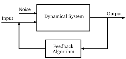
Figure 1: A diagrammatic depiction of the process of feedback control. The output of the noisy dynamical system is monitored. The resulting measured signal is processed by a device which calculates the required input (the feedback) as a functional of this signal. The precise functional used is called the feedback algorithm. The goal of the feedback is often to minimize the effect of the noise on the dynamics of the system, but it can also be to modify the behavior of the system in some other way.

In what follows we will discuss a number of explicit examples of feedback control in a variety of quantum systems, and this will allow us to give specific examples of the dynamics induced by measurement. Before we examine such examples however, it is worth presenting the general equations which describe feedback control in quantum systems, in analogy to those for classical systems. In classical systems, the state-of-knowledge of someone observing the system is given by a probability density over the dynamical variables (a phase-space probability density). Let us consider for simplicity a single particle, whose dynamical variables are its position, $x$ and momentum, $p$. If the observer is continually monitoring the position of the particle, then her stream of measurement results, $r(t)$ is usually described well by

$$dr=x(t)dt+\frac{dV(t)}{\sqrt{\gamma}}\,,$$ (1)

where in each time interval $dt$, $dV(t)$ is a Gaussian random variable with variance $dt$ and a mean of zero. Such a Gaussian noise process is called Wiener noise . The constant $\gamma$ determines the relative size of the noise, and thus also the rate at which the measurement extracts information about $x$; when $\gamma$ is increased, the noise decreases, and it therefore takes the observer less time to obtain an accurate measurement of $x$.

As the observer obtains information, her state-of-knowledge regarding the system, $P(x,p)$, evolves. The evolution is given by the Kushner-Stratonovich (K-S) Equation. This is

$$dP=\left[-\frac{p}{m}\partial_{x}-F(x,t)\partial_{p}\right]Pdt+\sqrt{\gamma}(x-\langle x(t)\rangle)PdW,$$ (2)

where $m$ is the mass of the particle, $F(x,t)$ is the force on the particle,

$$\langle x(t)\rangle=\int_{-\infty}^{\infty}\int_{-\infty}^{\infty}\!\!\!\!x\,P(x,p)\;dxdp$$ (3)

is the expectation value of $x$ at time $t$, and

$$dW(t)=\sqrt{\gamma}(x-\langle x\rangle)dt+dV(t)$$ (4)

turns out to be a Wiener noise, uncorrelated with the probability density $P$. Because of this we can alternatively write the stream of measurement results as

$$dr=\langle x(t)\rangle dt+\frac{dW}{\sqrt{\gamma}}\,.$$ (5)

The above will no doubt be familiar to the majority of the readership. For linear dynamical systems the K-S equation reduces to the equations of the well-known Kalman-Bucy filter [1].

The K-S equation is the essential tool for describing feedback control; it tells us what the observer knows about the system at each point in time, and thus the information that he or she can use to determine the feedback forces at each point in time. In addition, when we include these forces in the system dynamics, the resulting K-S equation, in telling us the observer’s state-of-knowledge is also telling us how effective is our feedback control: the variance of this state-of-knowledge, and the fluctuations of its mean (note that these are two separate things) tell us the remaining uncertainty in the system. The K-S equation thus allows us to design and evaluate feedback algorithms.

The description of dynamics and continuous measurement in quantum mechanics is closely analogous to the classical case described above. In quantum mechanics, however, the observer’s state-of-knowledge must be represented by a matrix, rather than a probability density. This matrix is called the density matrix, and usually denoted by $\rho(t)$. The dynamical variables are also represented by matrices. If the position is represented by the matrix $X$, then the expectation value of the particle’s position at time $t$ is given by $\langle x(t)\rangle=\mbox{Tr}[\rho(t)X]$ [5]. While the notion that a state-of-knowledge is described by a matrix will appear very strange to most of the readership, don’t let this put you off — when we consider feedback control we will always discuss it in terms of standard physical quantities such as the expectation values, variances, or probability densities for the dynamical variables. The reason we speak of the density matrix as representing the observer’s state-of-knowledge is because all these quantities can be obtained directly from the density matrix.

The dynamics of an unobserved quantum system may be written as $i\hbar\dot{\rho}=[H,\rho]\equiv H\rho-\rho H$ for a given matrix $H$ called the Hamiltonian ($\hbar$ is Planck’s constant). If an observer makes a continuous measurement of a particle’s position, then the full dynamics of the observer’s state-of-knowledge is given by the quantum equivalent of the Kushner-Stratonovich equation. This is

$$d\rho = -\frac{i}{\hbar}[H,\rho]dt-(\gamma/8)[X,[X,\rho]]dt$$ (6)

$$+\frac{\sqrt{\gamma}}{2}((X-\langle x(t)\rangle)\rho+\rho(X-\langle x(t)\rangle))dW,$$

where the observer’s stream of measurement results is

$$dr=\langle x(t)\rangle dt+\frac{dW}{\sqrt{\gamma}}.$$ (7)

This is referred to as the Stochastic Master Equation (SME), and was first derived by Belavkin [6]. This is very similar to the K-S equation, but has the extra term $[X,[X,\rho]]$ that describes the noisy dynamics (or quantum back-action) which is introduced by the measurement. In the quantum mechanics literature the measurement rate $\gamma$ is often referred to as the measurement strength. The SME is usually derived directly from quantum measurement theory [7, 8] without using the mathematical machinery of filtering theory. A recent derivation for people familiar with filtering theory may be found in [9]. Armed with the quantum equivalent of the K-S equation, we can proceed to consider feedback control in quantum systems.

Interpreting “applications of feedback control in quantum systems” in a broad sense, it would appear that one can break most such applications into three general classes. While these classes may be somewhat artificial, they are a useful pedagogical tool, and we will focus on specific examples from each group in turn in the following three sections. The first group is the application of results and techniques from classical control theory to the general theory of the control of quantum systems. This includes the application control theory to obtain optimal control algorithms for special classes of quantum systems. An example of this is the realization that classical LQG control theory can be applied directly to obtain optimal control algorithms for observed linear quantum systems [6, 12, 10]. We will discuss this and other examples in Section II.

It is worth noting at this point that while the direct application of classical control theory to quantum systems is very useful, it is not the only approach to understanding the design of feedback algorithms in quantum systems. Another approach is to try to gain insights into the relationship between measurement (information extraction) and disturbance in quantum mechanics which are relevant to feedback control. Such questions are also of fundamental interest to quantum theorists since they help to elucidate the information theoretic structure of quantum mechanics. References [13] and [14] take this approach, elucidating the information-disturbance trade-off relations for a two-state system (the simplest non-linear quantum system), and exploring the effects of this on the design of feedback algorithms.

The second group is the application of feedback control to classes of control problems which arise in quantum systems, some of which are analogous to those in classical systems, and some of which are peculiar to quantum systems. A primary example of this is in adaptive measurement, where feedback control is used during the measurement process to change the properties of the measurement. This is usually for the purpose of increasing the information which the measurement obtains about specific quantities, or increasing the rate at which information is obtained. We will discuss such applications in Section III.

The third group is the design and application of feedback algorithms to control specific quantum systems. Examples are applications to the cooling of a nano-mechanical resonator and the cooling of a single atom trapped in an optical cavity. We will discuss these in Section IV.

II Optimal Control for Linear Quantum Systems

Most readers of this article will certainly be familiar with the classical theory of optimal Linear-Quadratic-Gaussian (LQG) control. This provides optimal feedback algorithms for linear systems driven by Gaussian noise, and in which the observer monitors some linear combination of the dynamical variables. In LQG control, the control objective is the minimization of a quadratic function of the dynamical variables (such as the energy). It turns out that for a restricted class of observed quantum systems (those which are linear in a sense to be defined below), this optimal control theory can be applied directly. This was first realized by Belavkin in [6], and later independently by Yanagisawa and Kimura [12] and Doherty and Jacobs [10].

Quantum mechanical systems whose Hamiltonians are no more than quadratic in the dynamical variables are referred to as linear quantum systems, since the equations of motion for the matrices representing the dynamical variables are linear. Further, these linear equations are precisely the same as those for a classical system subject to the same forces. The simplest example is the Harmonic oscillator. If we denote the matrices for position and momentum as $X$ and $P$ respectively, then the Hamiltonian is

$$H=\frac{P^{2}}{2m}+\frac{1}{2}m\omega^{2}X^{2}$$ (8)

where $m$ is the mass of the particle, and $\omega$ is the angular frequency with which it oscillates. The resulting equations for $X$ and $P$ are

$$\dot{X} = P/m$$ (9)

$$\dot{P} = -m\omega X,$$ (10)

which are of course identical to the classical equations for the dynamical variables $x$ and $p$ in a classical harmonic oscillator. Further, it turns out that if an observer makes a continuous measurement of any linear combination of the position and momentum, then the SME for the observer’s state of knowledge of the quantum system reduces to the Kushner-Stratonovich equation, which in this case, because the system is linear, is simply the Kalman-Bucy Filter Equations.

However, there is one twist. The Kalman-Bucy equations one obtains for the quantum system are those for a classical harmonic oscillator driven by Gaussian noise of strength $\hbar\gamma$. This comes from the extra term in the SME which describes the “quantum back-action” noise generated by the measurement. Since the observer’s state of knowledge evolves in precisely the same way as for the equivalent linear classical system, albeit driven by noise, we can apply classical LQG theory to these quantum systems. If we apply linear feedback forces, then, for a fixed measurement strength $\gamma$, the quantum mechanics will tell us how much noise the system is subject to, and LQG theory will tell us the resulting optimal feedback algorithm for a given quadratic control objective [6, 10].

Note however, that since the noise driving the system depends upon the strength of the measurement, then the performance of the feedback algorithm will also depend upon the strength of the measurement. Moreover, the performance of the algorithm will be influenced by two competing effects: as the measurement gets stronger, we can expect the algorithm to do better as a result of the fact that the observer is more rapidly obtaining information. However, as the measurement gets stronger, the induced noise also increases, which will reduce the effectiveness of the algorithm. We can therefore expect that there will be an optimal measurement strength at which the feedback is most effective. In a linear quantum system one therefore must first find the optimal feedback algorithm using LQG control theory, and then perform a second optimization over the measurement strength. This is not the case in classical control. An explicit example of optimizing measurement strength may be found in [15].

The application of LQG theory to linear quantum systems will be useful when we examine the control of a nanomechanical resonator in Section IV. The close connection between linear quantum and classical systems allows one to apply other results from classical control theory for linear systems to quantum linear systems. Transfer function techniques have been applied to linear quantum systems by Yanagisawa and Kimura [16, 17], and D’Helon and James have elucidated how the small gain theorem can be applied to linear quantum optical networks [18]. Finally, it is possible to obtain exact results for the control of linear quantum systems for at least one case beyond LQG theory: James has extended the theory of risk-sensitive control to linear quantum systems [19].

For nonlinear quantum systems, naturally many of the approaches developed for classical non-linear systems can be expected to be useful. A few specific applications of methods developed for classical nonlinear systems have been explored to date. One example is the use of linearization to obtain control algorithms [11], and another is the application of a classical guidance algorithm to the control of a quantum system [20]. A third example is the application of the projection filter technique to obtain approximate filters for continuous state-estimation of nonlinear quantum optical systems [21]. The Bellman equation has also been investigated for a two-state quantum system in [22]; it is not possible to obtain a general analytic solution to this equation for such a system, and as yet no-one has attempted to solve this problem numerically. As quantum systems become increasingly important in the development of technologies, no doubt many more techniques and results from non-linear control theory will be applied in such systems.

III Adaptive Measurement

The objective of LQG control is to use feedback to minimize some quadratic function of the dynamical variables, and this is natural if one wishes to maintain a desired behavior in the presence of noise. While stabilization and noise reduction in dynamical systems is a very important application of feedback control, it is by no means the only application. Another important class of applications is adaptive measurement.

An adaptive measurement is one in which the measurement is altered as information is obtained. That is, a process of feedback is used to alter the measurement as it proceeds, rather than altering the system The primary distinction between adaptive measurement and more traditional control objectives however is that the goal of the former is usually to optimize some property of the information obtained in the measurement process rather than to control the dynamics of the system.

Adaptive measurement has, even at this relatively early stage in the development of the field of quantum feedback control, found many potential applications in quantum systems. The reason for this is due to the interplay of the following things. The first is that unlike classical states the majority of quantum states are not fully distinguishable from each other, even in theory, and only carefully chosen measurements will optimally distinguish between a given set of states. The second is that because quantum measurements generally disturb the system being measured, one must also choose one’s measurements very carefully in order to extract the maximal information about a given quantity (lest the measurement disturb this quantity). Combining these two things with the fact that one is usually limited in the kinds of measurements one can perform, due to the available physical interactions between a given system and measuring devices, it is frequently impossible to implement optimal measurements in quantum systems. The use of adaptive measurement increases the range of possible measurements one can make in a given physical situation, and in some cases allows optimal measurements to be constructed where they could not be otherwise.

III-A State-Discrimination and Parameter Estimation

As far as the author is aware, the first application of quantum adaptive measurement was introduced by Dolinar in 1973 [23, 24]. Here the problem involves communicating with a laser beam, where each bit is encoded by the presence or absence of a pulse of laser light. Quantum effects become important when the average number of photons in each pulse is small (e.g. $\leq 10$). In fact, it is not possible to completely distinguish between the presence or absence of a pulse. The reason for this is that the quantum nature of the pulse of laser light is such that there is always a finite probability that there are no photons in the pulse. It turns out that the optimal way of distinguishing the two states is by mixing the pulse with another laser beam at a beam splitter, and detecting the resulting combined beam. In this case both input states will produce photon clicks. The optimal procedure is to vary the amplitude of the mixing beam with time, and in particular to use a process of feedback to change this amplitude after the detection of each photon. This feedback procedure distinguishes the states maximally well within the limits imposed by quantum mechanics (referred to as the Helstrom bound [25]).

The objective of Dolinar’s adaptive measurement scheme is to discriminate maximally well between two states. Alternatively one may wish to discriminate maximally fast. To put this another way, one may wish to maximize the amount of information which is obtained in a specified time, even if it is not possible to obtain all the information in that time. Such considerations can be potentially useful in optimizing information transmission rates when the time taken to prepare the states is significant. In [26] it is shown that adaptive measurement can be used to increase the speed of state-discrimination. Of particular interest in quantum control theory are situations which reveal differences between measurements on quantum systems and those on their classical counterparts. The rapid-discrimination adaptive measurement scheme of [26] is one such example. The reason for this is that in the case considered in [26] it is only possible to use an adaptive algorithm to increase the speed of discrimination if quantum mechanics forbids perfect discrimination between them. Since all classical states are completely distinguishable (at least in theory), this adaptive measurement is only applicable to quantum systems. The question of whether or not there are more general situations which provide classical analogues of this adaptive measurement is an open question, however.

The problem of quantum state-discrimination is a special case of parameter estimation. In parameter estimation, the possible states that a system could have been prepared in (or alternatively the possible Hamiltonians that may describe the dynamics of a system) are parametrized in some way. The observer then tries to determine the value of the parameter by measuring the system. When discriminating two states the parameter has only two discrete values: in the above case it is the amplitude of the laser pulse, which is either zero or non-zero. In a more general case one wishes to determine a continuous parameter. An example of this is the detection of a force. In this case a simple system which feels the force, such as a quantum harmonic oscillator, is monitored, and the force is determined from the observed dynamics. Two examples of this are the atomic force microscope (AFM) [27] and the detection of gravitational waves [28]. Adaptive measurement is useful in parameter estimation because measurements which are not precisely tailored will disturb the system so as to degrade information about the parameter. To the author’s knowledge no-one has yet investigated adaptive measurement in force estimation, although the subject is discussed briefly in [29]. However, the use of adaptive measurement for the estimation of a magnetic field using a cold atomic cloud has been investigated in [30, 31], and for the estimation of a phase shift imparted on a light beam has been explored in references [32, 33, 34]. In [34] the authors show that adaptive measurement outperforms other known kinds of measurements for estimation of phase shifts on continuous beams of light.

III-B Constructing New Measurements

It turns out that there are certain kinds of measurements which it is very difficult to make because the necessary interactions between the measurement device and the system are not easily engineered. One such example in quantum mechanics is a measurement of what is referred to as the “Pegg-Barnett” or “canonical” phase [35]. There are subtleties in defining what one means by the phase of a quantum mechanical light beam (or, more precisely, in obtaining a definition with all the desired properties). Astonishingly, the question was not resolved until 1988, when Pegg and Barnett constructed a definition which has the desired properties for all practical purposes. This is called the canonical phase of a light beam.

Now, the most practical method of measuring light is to use a photon counter. However, it turns out that it is not possible to use a photon counter, even indirectly, to make a measurement which measures precisely canonical phase Nevetheless, in [37] (see also [38, 39]) Wiseman showed that the use of an adaptive measurement process allows one to more closely approximate a canonical phase measurement. For a light pulse which has at most one photon, this adaptive phase measurement measures precisely canonical phase. Wiseman’s adaptive phase measurement has now been realized experimentally [40].

III-C Rapid State-Preparation

One application of feedback control is in preparing quantum systems in well-defined states. Due to noise from the environment, the state of quantum systems which have been left to their own devices for an appreciable time will contain considerable uncertainty. Many quantum devices, for example those proposed for information processing [41], require that the quantum system be prepared in a state which is specified to high precision. Naturally one can prepare such states by using measurement followed by control - that is, using a measurement to determine the state to high precision, and then applying a control field to move the system to the desired point in phase space.

Since the rate at which a given measuring device will extract information is always finite, one can ask whether it is possible to increase the rate at which information is extracted by using a process of adaptive measurement. That is, to adaptively change the measurement as the observer’s state-of-knowledge changes, so that the uncertainty (e.g. the entropy) of the observer’s state-of-knowledge reduces faster. We will refer to the process of reducing the entropy as purifying the qubit (a term taken from the jargon of quantum mechanics). It turns out that it is indeed possible to increase the rate of purification using adaptive measurement.

For a two-state quantum system (often referred to as a qubit), an adaptive measurement is presented in [42] that will speed-up the rate of purification in a certain sense. Specifically, it will increase the rate of reduction of the average entropy of the qubit (where the average is taken over the possible realizations of the measurement - e.g. over measurements on many identical qubits) by a factor of two. This adaptive measurement has two further interesting properties. The first is that there is no analogous adaptive scheme for the equivalent measurement on a classic two-state system (a single bit); the speed-up in the reduction of the average entropy is a quantum mechanical effect.

The second property has to do with the statistics of the entropy reduction. For a fixed measurement, while the entropy decreases with time on average, on any given realization of the measurement the entropy fluctuates randomly as measurement proceeds. For the adaptive measurement however, in the limit of strong feedback, the entropy reduces deterministically. For a finite feedback force, there will always remain some residual stochasticity in the entropy reduction, but this will be reduced over that for the fixed measurement [42, 43]. Thus if one is preparing many qubits in parallel, this adaptive measurement will reduce the spread in the time it takes the qubits to be prepared.

The above adaptive algorithm does not speed up purification in every sense of the word, however: Wiseman and Ralph [44] have recently shown that while the above adaptive measurement reduces the average entropy of an ensemble of qubits more quickly, quite surprisingly it actually increases the average time it takes to prepare a given value of the entropy by a factor of two! In this sense, therefore, the above measurement strategy does not, in fact, speed up preparation. The reason for this is that when one considers an ensemble of spins, the majority purify quickly, whereas the average value of the entropy across the ensemble is increased considerably by a small number of straggling qubits that purify slowly. Thus, the adaptive measurement works by decreasing the time taken for the stragglers, but increasing the time taken for the majority, so that, for strong feedback, all qubits take the same time to reach a given purity. Thus the feedback algorithm constructed in [42] does not speed up the average time a given qubit will take to reach a target entropy, and this will be the important quantity if one is preparing qubits in sequence. Application of the above results to rapid purification of superconducting qubits is analyzed in [45, 46].

Is it possible, therefore, to use adaptive measurement to speed up the average preparation time? While the answer for a single qubit is almost certainly no, the answer is almost certainly yes in general: In [47] the authors show that, for a quantum system with $N$ states it is possible to speed up the rate at which the average entropy is reduced by a factor proportional to $N$. While it is not shown directly that this algorithm also decreases the average time to reach a given target purity, it is fairly clear that this will be the case, although more work remains to be done before all the answers are in.

Another application of feedback control involving purification of states has been explored in [48, 49]. In this case, rather than the rate of purification, the authors are concerned with using feedback control during the measurement to obtain a specific final state, and in particular when the control fields are restricted.

In this section we have been considering the application of feedback in quantum systems to problems which lie outside the traditional applications of noise reduction and stabilization. Most of these fall under the category of adaptive measurement, and these we have discussed above. One that does not is quantum error correction. The goal of such a process is noise reduction, but with the twist that the state of the system must be encoded in such a way that the controller does not disturb the information in the system. While we will not discuss this further here, the interested reader is referred to [50, 51, 52] and references therein.

IV Controlling Nanoscopic Systems

We now present examples of feedback control applied to two specific quantum systems. The first is a nano-mechanical resonator, and the second is a single atom trapped in an optical cavity. In both cases the goal of the feedback algorithm will be to reduce the entropy of the system and prepare it in its ground state. A nano-mechanical resonator is a thin, fairly ridged bridge, perhaps 200 nm wide and a few microns long. Such a bridge is formed on a layered wafer by etching out the layer beneath. If one places a conducting strip along the bridge and passes a current through it, the bridge can be made to vibrate like a guitar string by driving it with a magnetic field. So long as the amplitude of the oscillation is relatively small, the dynamics is essentially that of a harmonic oscillator [53]. One of the primary goals of research in this area is to observe quantum behavior in these oscillators [54]. The first step in such a process is to reduce the thermal noise which the oscillator is subject to in order to bring it close to its ground state.

Typical nanomechanical resonators have frequencies of the order of tens of megahertz. This means that to cool the resonator so that its average energy corresponds to its first excited state requires a temperature of a few milliKelvin. Dilution refrigerators can obtain temperatures of a few hundred milliKelvin, but to reduce the temperature further requires something else. In reference [55] the authors show that, at least in theory, feedback control could be used to obtain the required temperatures.

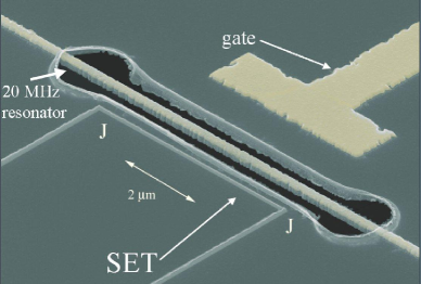
Figure 2: The nanomechanical resonator is a long thin bridge formed on a layered wafer by etching out the substrate beneath it. The bridge is driven with a magnetic field, and oscillates up and down at $20\mbox{MHz}$. On the near side of the resonator is a single electron transistor (SET), whose central island is formed by the two junctions marked “J”. On the far side is a T-Shaped electrode or “gate”. The voltage on this gate is varied and this results in a varying force on the resonator. Image courtesy of Keith Schwab.

To perform feedback control one must have a means of monitoring the position of the resonator and applying a feedback force. The position can be monitored using a single electron transistor, and this has recently been achieved experimentally [56]. A feedback force can be applied by varying the voltage on a gate placed adjacent to the resonator. This configuration is depicted in Figure 2. Since the oscillator is harmonic, classical LQG theory can be used to obtain an optimal feedback algorithm for minimizing the energy of the resonator, so long as one takes into account the quantum back-action noise caused by the measurement as described in [10]. The details involved in obtaining the optimal feedback algorithm and calculating the optimal measurement strength are given in [55]. It has further been shown in [57] that adaptive measurement and feedback can be used to prepare the resonator in a squeezed state.

The second example of feedback control we consider is that of cooling an atom trapped in an optical cavity. An optical cavity consists of two parallel mirrors with a single laser beam bouncing back and forward between them. The laser beam forms a standing wave between the mirrors, and if the laser frequency is chosen appropriately, a single atom inside the cavity will feel a sinusoidal potential due its interaction with the standing wave. It is therefore possible to trap an atom in one of the wells of this potential. It turns out that information regarding the position of the atom can be obtained by monitoring the phase of the light which leaks out one of the mirrors. Specifically, the phase of the output light tells the observer how far up the side of a potential well the atom is. In addition, by changing the intensity of the laser beam that is driving the cavity, one changes the height of the standing wave, and thus the height of the potential wells. In this system we therefore have a means to monitor the atom and to apply a feedback force. In [58, 59] the authors present a feedback algorithm which can be used to cool the atom to its ground state. Actually, the algorithm will prepare the atom either in its ground state, or its first excited state, each with a probability of $50\%$. However, from the measurement record the observer know which one, and can take appropriate action if the resulting state is not the desired one.

If the location of the atom was known very accurately, then we could use the following feedback algorithm to reduce its energy: increase the height of the potential when the atom is climbing up the side of a well, and reduce it when the atom is falling down towards the centre. This way the energy of the atom is reduced on each oscillation, and the atom will eventually be stationary at the centre of the well. However, it turns out that this algorithm is not effective, either classically or quantum mechanically, when the variance of atom in phase space is appreciable. The reason is that the cyclic process of raising and lowering the potential, which reduces the energy of the atom’s mean position and momentum, actually increases the variance of the phase-space probability density. Classically we can eliminate this problem by observing the atom with sufficient accuracy, but quantum mechanically Heisenberg’s uncertainty relation prevents us from reducing the variance sufficiently. As a result, an alternative algorithm is required.

If turns out that one can obtain an effective cooling algorithm by calculating the derivative of the total motional energy of the atom with respect to changes in the height of the potential. In doing so one finds that the energy change is maximal and minimal at a certain points in the oscillatory motion of the atom. As a result, one can use a bang-bang algorithm to switch the potential high when the energy reduction is maximal, and switch it low when the resulting energy increase is minimal, in a similar fashion to the classical algorithm described above. The result is that the atom will lose motional energy on each cycle.

The curious effect whereby the atom will cool to the ground state only half the time is due to the symmetry of the system, and the fact that the feedback algorithm respects this symmetry. Specifically, the feedback process cannot change the average parity of the initial probability density. Since the ground state has even parity, and the first excited state odd parity, if the initial density of the atom has no particular parity (a reasonable assumption), then to preserve this on average the process must pick even and odd final states equally often. Full details regarding the feedback algorithm and the resulting dynamics of the atom is given in [58, 59].

Although we do not have the space to describe them here, applications of feedback control have been proposed in a variety of other quantum systems. Three of these are cooling the motion of a cavity mirror by modulating the light in the cavity [60], controlling the motion of quantum-dot qubits [61], and preparing spin-squeezed states in atomic clouds [62]. In addition, feedback control has now been experimentally demonstrated in a number of quantum systems. Namely in optics [40, 63], cold atom clouds [64], and trapped ions [65].

V Conclusion

To summarize, feedback control has a wide variety of applications in quantum systems, particularly in the areas of noise reduction, stabilization, cooling and precision measurement. Such applications can be expected to grow more numerous as quantum systems become important as the basis of new technologies. While exact results from modern control theory can be used to obtain optimal control algorithms for some quantum systems, this is not true for the majority of quantum control problems due to their inherent non-linearity. As a result many techniques developed for the control of nonlinear classical systems are of considerable use in designing algorithms for quantum feedback control, and the efficacy of many of these techniques still remain to be explored in quantum systems. Hopefully as further quantum control problems arise in specific systems, and effective control algorithms are developed, rules of thumb will emerge for the control of classes of quantum devices.

References

- [1] P. S. Maybeck, Stochastic Models, Estimation and Control. Academic Press, New York, 1982, vol. I and II.
- [2] P. Whittle, Optimal Control. Wiley & Sons, Chichester, 1996.
- [3] D. T. Gillespie, “The mathematics of brownian motion and johnson noise,” Am. J. Phys., vol. 64, p. 225, 1996.
- [4] K. Jacobs, “Topics in quantum measurement and quantum noise,” Ph.D. dissertation, Imperial College, London, 1998.
- [5] J. J. Sakuri, Modern Quantum Mechanics. Addison-Wesley, San Francisco, 1994.
- [6] V. P. Belavkin, “Non-demolition measurement and control in quantum dynamical systems,” in Information, Complexity and Control in Quantum Physics, A. Blaquiere, S. Diner, and G. Lochak, Eds. Springer-Verlag, New York, 1987.
- [7] H. M. Wiseman and G. J. Milburn, “Quantum theory of field-quadrature measurements,” Phys. Rev. A, vol. 47, p. 642, 1993.
- [8] T. A. Brun, “A simple model of quantum trajectories,” American Journal of Physics, vol. 70, p. 719, 2002.
- [9] L. Bouten, R. van Handel, and M. James, “An introduction to quantum filtering,” Eprint: math.OC/0601741.
- [10] A. C. Doherty and K. Jacobs, “Feedback control of quantum systems using continuous state estimation,” Phys. Rev. A, vol. 60, p. 2700, 1999.
- [11] A. C. Doherty, S. Habib, K. Jacobs, H. Mabuchi, and S. M. Tan, “Quantum feedback control and classical control theory,” Phys. Rev. A, vol. 62, p. 012105, 2000.
- [12] M. Yanagisawa and H. Kimura, in Learning, Control and Hybrid Systems, Lecture Notes in Control and Information Sciences. Springer-Verlag, New York, 1998, vol. 241, p. 249.
- [13] C. A. Fuchs and K. Jacobs, “Information-tradeoff relations for finite-strength quantum measurements,” Phys. Rev. A, vol. 63, p. 062305, 2001.
- [14] A. C. Doherty, K. Jacobs, and G. Jungman, “Information, disturbance, and hamiltonian quantum feedback control,” Phys. Rev. A, vol. 63, p. 062306, 2001.
- [15] A. C. Doherty and H. M. Wiseman, “Quantum limits to feedback control of linear systems,” P. Heszler, Ed., vol. 5468, no. 1. SPIE, 2004, p. 322.
- [16] M. Yanagisawa and H. Kimura, “Transfer function approach to quantum control-part i: Dynamics of quantum feedback systems,” IEEE Trans. Automat. Contr., vol. 48, p. 2107, 2003.
- [17] ——, “Transfer function approach to quantum control-part ii: Control concepts and applications,” IEEE Trans. Automat. Contr., vol. 48, p. 2121, 2003.
- [18] C. D’Helon and M. R. James, “Stability, gain, and robustness in quantum feedback networks,” Eprint: quant-ph/0511140.
- [19] M. R. James, “Risk-sensitive optimal control of quantum systems,” Phys. Rev. A, vol. 69, p. 032108, 2004.
- [20] J. F. Ralph, E. J. Griffith, T. D. Clark, and M. J. Everitt, “Guidance and control in a josephson charge qubit,” Phys. Rev. B, vol. 70, p. 214521, 2004.
- [21] R. van Handel and H. Mabuchi, “Quantum projection filter for a highly nonlinear model in cavity qed,” J. Opt. B: Quantum Semiclass. Opt., vol. 7, p. S226, 2005.
- [22] L. Bouten, S. Edwards, and V. P. Belavkin, “Bellman equations for optimal feedback control of qubit states,” J. Phys. B: At. Mol. Opt. Phys., vol. 38, p. 151, 2005.
- [23] S. Dolinar, Tech. Rep. 111, Research Laboratory of Electronics. MIT, Cambridge, 1973.
- [24] J. Geremia, “Distinguishing between optical coherent states with imperfect detection,” Phys. Rev. A, vol. 70, p. 062303, 2004.
- [25] C. W. Helstrom, Quantum Detection and Estimation Theory, ser. Mathematics in Science and Egineering. Academic Press, New York, 1976, vol. 123.
- [26] K. Jacobs, “Feedback control for communication with non-orthogonal states,” Eprint: quant-ph/0601162.
- [27] G. J. Milburn, K. Jacobs, and D. F. Walls, “Quantum-limited measurements with the atomic force microscope,” Phys. Rev. A, vol. 50, no. 6, p. 5256, 1994.
- [28] V. B. Braginsky, M. L. Gorodetsky, F. Y. Khalili, A. B. Matsko, K. S. Thorne, and S. P. Vyatchanin, “Noise in gravitational-wave detectors and other classical-force measurements is not influenced by test-mass quantization,” Phys. Rev. D, vol. 67, no. 8, p. 082001, 2003.
- [29] F. Verstraete, A. C. Doherty, and H. Mabuchi, “Sensitivity optimization in quantum parameter estimation,” Phys. Rev. A, vol. 64, p. 032111, 2001.
- [30] J. K. Stockton, J. M. Geremia, A. C. Doherty, and H. Mabuchi, “Robust quantum parameter estimation: Coherent magnetometry with feedback,” Phys. Rev. A, vol. 69, p. 032109, 2004.
- [31] J. Geremia, J. K. Stockton, and H. Mabuchi, “Suppression of spin projection noise in broadband atomic magnetometry,” Physical Review Letters, vol. 94, p. 203002, 2005.
- [32] D. W. Berry, H. M. Wiseman, and J. K. Breslin, “Optimal input states and feedback for interferometric phase estimation,” Phys. Rev. A, vol. 63, p. 053804, 2001.
- [33] D. W. Berry and H. M. Wiseman, “Adaptive quantum measurements of a continuously varying phase,” Physical Review A, vol. 65, p. 043803, 2002.
- [34] D. T. Pope, H. M. Wiseman, and N. K. Langford, “Adaptive phase estimation is more accurate than nonadaptive phase estimation for continuous beams of light,” Physical Review A, vol. 70, p. 043812, 2004.
- [35] D. T. Pegg and S. M. Barnett, “Unitary phase operator in quantum mechanics,” Europhysics Lett., vol. 6, p. 483, 1988.
- [36] K. L. Pregnell and D. T. Pegg, “Single-shot measurement of quantum optical phase,” Eprint: quant-ph/0506206.
- [37] H. M. Wiseman, “Adaptive phase measurements of optical modes: Going beyond the marginal q distribution,” Phys. Rev. Lett., vol. 75, p. 4587, 1995.
- [38] H. M. Wiseman and R. B. Killip, “Adaptive single-shot phase measurements: A semiclassical approach,” Phys. Rev. A, vol. 56, p. 944, 1997.
- [39] ——, “Adaptive single-shot phase measurements: The full quantum theory,” Phys. Rev. A, vol. 57, p. 2169, 1998.
- [40] M. A. Armen, J. K. Au, J. K. Stockton, A. C. Doherty, and H. Mabuchi, “Adaptive homodyne measurement of optical phase,” Phys. Rev. Lett., vol. 89, p. 133602, 2002.
- [41] T. P. Spiller, W. J. Munro, S. D. Barrett, and P. Kok, “An introduction to quantum information processing: applications and realizations,” Cont. Phys., vol. 46, p. 407, 2005.
- [42] K. Jacobs, “How to project qubits faster using quantum feedback,” Phys. Rev. A, vol. 67, p. 030301(R), 2003.
- [43] ——, “Optimal feedback control for rapid preparation of a qubit,” P. Heszler, Ed., vol. 5468, no. 1. SPIE, 2004, p. 355.
- [44] H. M. Wiseman and J. F. Ralph, “Reconsidering rapid qubit purification by feedback,” Eprint: quant-ph/0603062.
- [45] J. F. Ralph, E. J. Griffith, and C. D. H. A. D. Clark, “Rapid purification of a solid state charge qubit,” E. J. Donkor, A. R. Pirich, and H. E. Brandt, Eds., vol. 6244. SPIE, 2006, p. (in press).
- [46] E. J. Griffith, C. D. Hill, J. F. Ralph, and K. Jacobs, “Rapid state purification in a superconducting charge qubit,” (in preparation).
- [47] J. Combes and K. Jacobs, “Rapid state-reduction of quantum systems using feedback control,” Phys. Rev. Lett., vol. 96, p. 010504, 2006.
- [48] J. K. Stockton, R. van Handel, and H. Mabuchi, “Deterministic dicke-state preparation with continuous measurement and control,” Phys. Rev. A, vol. 70, p. 022106, 2004.
- [49] R. van Handel, J. K. Stockton, and H. Mabuchi, “Feedback control of quantum state reduction,” IEEE Trans. Automat. Control, vol. 50, p. 768, 2005.
- [50] C. Ahn, A. C. Doherty, and A. J. Landahl, “Continuous quantum error correction via quantum feedback control,” Physical Review A (Atomic, Molecular, and Optical Physics), vol. 65, p. 042301, 2002.
- [51] M. Sarovar, C. Ahn, K. Jacobs, and G. J. Milburn, “Practical scheme for error control using feedback,” Physical Review A (Atomic, Molecular, and Optical Physics), vol. 69, p. 052324, 2004.
- [52] C. Ahn, H. Wiseman, and K. Jacobs, “Quantum error correction for continuously detected errors with any number of error channels per qubit,” Phys. Rev. A, vol. 70, p. 024302, 2004.
- [53] M. P. Blencowe, “Quantum electromechanical systems,” Phys. Rep., vol. 395, p. 159, 2004.
- [54] A. Cho, “Researchers race to put the quantum into mechanics,” Science, vol. 299, no. 5603, p. 36, 3 January 2003.
- [55] A. Hopkins, K. Jacobs, S. Habib, and K. Schwab, “Feedback cooling of a nanomechanical resonator,” Phys. Rev. B, vol. 68, p. 235328, 2003.
- [56] M. D. LaHaye, O. Buu, B. Camarota, and K. C. Schwab, “Approaching the quantum limit of a nanomechanical resonator,” Science, vol. 304, p. 74, 2004.
- [57] R. Ruskov, K. Schwab, and A. N. Korotkov, “Squeezing of a nanomechanical resonator by quantum nondemolition measurement and feedback,” Phys. Rev. B, vol. 71, p. 235407, 2005.
- [58] D. Steck, K. Jacobs, H. Mabuchi, T. Bhattacharya, and S. Habib, “Quantum feedback control of atomic motion in an optical cavity,” Phys. Rev. Lett., vol. 92, p. 223004, 2004.
- [59] D. Steck, K. Jacobs, H. Mabuchi, S. Habib, and T. Bhattacharya, “Feedback cooling of atomic motion in cavity qed,” Eprint: quant-ph/0509039.
- [60] S. Mancini, D. Vitali, and P. Tombesi, “Optomechanical cooling of a macroscopic oscillator by homodyne feedback,” Phys. Rev. Lett., vol. 80, p. 688, 1998.
- [61] R. Ruskov and A. N. Korotkov, “Quantum feedback control of a solid-state qubit,” Phys. Rev. B, vol. 66, p. 041401, 2002.
- [62] L. K. Thomsen, S. Mancini, and H. M. Wiseman, “Spin squeezing via quantum feedback,” Phys. Rev. A, vol. 65, p. 061801, 2002.
- [63] W. P. Smith, J. E. Reiner, L. A. Orozco, S. Kuhr, and H. M. Wiseman, “Capture and release of a conditional state of a cavity qed system by quantum feedback,” Phys. Rev. Lett., vol. 89, p. 133601, 2002.
- [64] J. M. Geremia, J. K. Stockton, and H. Mabuchi, “Real-time quantum feedback control of atomic spin-squeezing,” Science, vol. 304, p. 270, 2004.
- [65] P. Bushev, D. Rotter, A. Wilson, F. Dubin, C. Becher, J. Eschner, R. Blatt, V. Steixner, P. Rabl, and P. Zoller, “Feedback cooling of a single trapped ion,” Phys. Rev. Lett., vol. 96, p. 043003, 2006.