Potential and limits to cluster state quantum computing using probabilistic gates

Abstract

We establish bounds to the necessary resource consumption when building up cluster states for one-way computing using probabilistic gates. Emphasis is put on state preparation with linear optical gates, as the probabilistic character is unavoidable here. We identify rigorous general bounds to the necessary consumption of initially available maximally entangled pairs when building up one-dimensional cluster states with individually acting linear optical quantum gates, entangled pairs and vacuum modes. As the known linear optics gates have a limited maximum success probability, as we show, this amounts to finding the optimal classical strategy of fusing pieces of linear cluster states. A formal notion of classical configurations and strategies is introduced for probabilistic non-faulty gates. We study the asymptotic performance of strategies that can be simply described, and prove ultimate bounds to the performance of the globally optimal strategy. The arguments employ methods of random walks and convex optimization. This optimal strategy is also the one that requires the shortest storage time, and necessitates the fewest invocations of probabilistic gates. For two-dimensional cluster states, we find, for any elementary success probability, an essentially deterministic preparation of a cluster state with quadratic, hence optimal, asymptotic scaling in the use of entangled pairs. We also identify a percolation effect in state preparation, in that from a threshold probability on, almost all preparations will be either successful or fail. We outline the implications on linear optical architectures and fault-tolerant computations.

I Introduction

Optical quantum systems offer a number of advantages that render them suitable for attempting to employ them in architectures for a universal quantum computer: decoherence is less of an issue for photons compared to other physical systems, and many of the tools necessary for quantum state manipulation are readily available [1, 2, 3, 4, 5, 6, 7]. Also, the possibility of distributed computation is an essentially built-in feature [7, 8, 9]. Needless to say, any realization of a medium-scale linear optical quantum computer still constitutes an enormous challenge [10]. In addition to the usual requirement of near-perfect hardware components – here, sources of single photons or entangled pairs, linear optical networks, and photon detectors – one has to live with a further difficulty inherent in this kind of architecture: due to the small success probability of elementary gates, a very significant overhead in optical elements and additional photons is required to render the overall protocol near-deterministic.

Indeed, as there are no photon-photon interactions present in coherent linear optics, all non-linearities have to be induced by means of measurements. Hence, the probabilistic character is at the core of such schemes. It was the very point of the celebrated work of Ref. [1] that near-deterministic quantum computation is indeed possible using quantum gates (here: non-linear sign shift gates) that operate with a very low probability of success: only one quarter. Ironically, it turned out later that this value cannot be improved at all within the setting of linear optics without feed-forward [11]. Essentially due to this small probability, an enormous overhead in resources in the full scheme involving feed-forward is needed.

There is, fortunately, nevertheless room for a reduction of this overhead, based on this seminal work. Recent years saw a development reminiscent of a “Moore’s law”, in that each year, a new scheme was suggested that reduced the necessary resources by a large factor. In particular, the most promising results have been achieved [3, 4, 5] by abandoning the standard gate model of quantum computation [10] in favor of the measurement-based one-way computer [12]. Taking resource consumption as a benchmark, the most recent schemes range more than two orders of magnitude below the original proposal. It is thus meaningful to ask: How long can this development be sustained? What are the ultimate limits to overhead reduction for linear optics quantum computation? The latter question was one of the main motivations for our work.

The reader is urged to recall that a computation in the one-way model proceeds in two steps. Firstly, a highly entangled cluster state [12, 13, 14, 15] is built up. Secondly, local measurements are performed on this state, the outcomes of which encode the result of the computation. As the ability to perform local measurements is part of the linear optical toolbox, the challenge lies solely in realizing the first step. More specifically, one- and two-dimensional cluster states can be built from EPR pairs [16] using probabilistic so-called fusion gates. In the light of this framework, the question posed at the end of the last paragraph takes on the form: measured in the number of required entangled pairs, how efficiently can one prepare cluster states using probabilistic fusion gates? There have been several proposals along these lines in recent years [3, 4, 5, 17, 18, 19, 20].

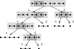
Figure 3: An example of a tree of successive configurations under application of a strategy. Light boxes group configurations. We start with $N=4$. Dark boxes indicate where the strategy decided to apply a fusion gate. Possible outcomes are success (to the left) or failure (to the right), resulting in different possible future choices. The expected length of the final chain is $\tilde{Q}_{M}(4)=Q(4)=13/8$.

It will be shown that the success probability of these gates can not be pushed beyond the currently known value of one half. Therefore, the only degree of freedom left in optimizing the process lies in adopting an optimal classical control strategy, which decides how the fusion gates are to be employed. This endeavor is greatly impeded by the gates’ probabilistic nature: the number of possible patterns of failure and success scales exponentially (see Fig. 3) and hence deciding how to optimally react to any of these situations constitutes a very hard problem indeed.

Maybe surprisingly, we find that classical control has tremendous implications concerning resource consumption (which seems particularly relevant when building up structures that render a scheme eventually fault-tolerant [21, 22]): even when aiming for moderate sized cluster states, one can easily reduce the required amount of entangled pairs by an order of magnitude when adopting the appropriate strategy. For the case of one-dimensional clusters, we identify a limit to the improvement of resource consumption by very tightly bounding from above the performance of any scheme which makes use of EPR pairs, vacuum modes and two-qubit quantum gates. In the two-dimensional setup, we establish that cluster states of size $n\times n$ can be prepared using $O(n^{2})$ input pairs.

We aim at providing a comprehensive study of the potential and limits to resource consumption for one-way computing, when the elementary gates operate in a non-faulty, but probabilistic fashion. As the work is phrased in terms of classical control strategies, it applies equally to the linear optical setting as to other architectures [17, 19, 23], such as those involving matter qubits and light as an entangling bus [24, 17]. This work extends an earlier report (Ref. [20]) where most ideas have already been sketched.

II Summary of results

Although the topic and results have very practical implications on the feasibility of linear optical one-way computing, we will have to establish a rather formal and mathematical setting in order to obtain rigorous results. To make these more accessible, we provide a short summary:

• We introduce a formal framework of classical strategies for building up linear cluster states. Linear cluster states can be pictured as chains of qubits, characterized by their length $l$ given in the number of edges. Maximally entangled qubit pairs correspond to chains with a single edge. By a configuration we mean a set of chains of specific individual lengths. Type-I fusion [5] allows for operations involving end qubits of two pieces (lengths $l_{1}$ and $l_{2}$), resulting on success in a single piece of length $l_{1}+l_{2}$ or on failure in two pieces of length $l_{1}-1$ and $l_{2}-1$. The process starts with a collection of $N$ EPR pairs and ends when only a single piece is left. A strategy decides which chains to fuse given a configuration. It is assessed by the expected length, or quality $\tilde{Q}(N)$ of the final cluster. The vast majority of strategies allow for no simple description and can be specified solely by a “lookup table” listing all configurations with the respective proposed action. Since the number of configurations scales exponentially as a function of the total number of edges $N$, a single strategy is already an extremely complex object and any form of brute force optimization is completely out of reach.

• After discussing the optimality of the primitive elementary physical gates, operating with a success probability of $p_{\text{s}}=1/2$, we start by studying the performance of several simple strategies. In particular, we study strategies which we refer to as Modesty and Greed:

  $$\text{\sc Greed}:$$ Always fuse the largest available

  linear cluster chains.

  $$\text{\sc Modesty}:$$ Always fuse the smallest available

  linear cluster chains

  in a configuration. Also, we investigate the strategy Static with a linear yield that minimizes the amount of sorting and feed-forward.

• We find that the choice of the classical strategy has a major impact on the resource consumption in the preparation of linear cluster states. When preparing cluster chains with an expected length of $40$, the number of required EPR pairs already differs by an order of magnitude when resorting to Modesty as compared to Greed.

• We provide an algorithm that symbolically identifies the globally optimal strategy, which yields the longest average chain with a given number $N$ of initially available EPR pairs. This globally optimal strategy can be found with an effort of $O(|{\cal C}^{(N)}|(\log|{\cal C}^{(N)}|)^{5})$. Here, $|{\cal C}^{(N)}|$ is the number of all configurations with up a total number of up to $N$ edges.

• We find that Modesty is almost globally optimal. For $N\leq 46$, the relative difference in the quality of the globally optimal strategy and Modesty is less than $1.1\times 10^{-3}$.

• Requiring significantly more formal effort, we provide fully rigorous proofs of tight analytical upper bounds concerning the quality of the globally optimal strategy. In particular, we find

  $$\tilde{Q}(N)\leq N/5+2.$$

  That is, frankly, within the setting of linear optics, in the sense made precise below, one has to invest at least five EPR pairs per average gain of one edge in the cluster state.

• A key step in the proof is the passage to a radically simplified model – dubbed razor model. Here, cluster pieces are cut down to a maximal length of two. While this step reduces the size of the configuration space tremendously, it retains – surprisingly – essential features of the problem. The whole problem can then be related to a random walk in a plane [25], and finally, to a convex optimization problem [26]. This bound constitutes the central technical result.

• The razor model also provides tools to get good numerical upper bounds with polynomial effort in $N$.

• Similarly, we find tight lower bounds for the quality, based on the symbolically available data for small values of $N$.

• We show that the questions (i) “given some fixed number of input pairs, how long a single chain can be obtained on average?” and (ii) “how many input pairs are needed to produce a chain of some fixed length with (almost) unity probability of success?” are asymptotically equivalent.

• For two-dimensional structures, we prove that one can build up cluster states with the optimal, quadratic use in resources, even when resorting to probabilistic gates: for any success probability $p_{\text{s}}\in(0,1]$ of the physical primitive quantum gate, one can prepare a $n\times n$ cluster state consuming $O(n^{2})$ EPR pairs. Previously known schemes have operated with a more costly scaling. This is possible in a way that the overall success probability $P_{\text{s}}(n)\rightarrow 1$ as $n\rightarrow\infty$. That is, even for quantum gates operating with a very small probability of success $p_{\text{s}}$, one can asymptotically deterministically build up two-dimensional cluster states using quadratically scaling resources.

• For this preparation, we observe an intriguing percolation effect when preparing cluster states using probabilistic gates: from a certain threshold probability

  $$p_{\text{s}}>p_{\text{th}}$$

  on, almost all preparations of a $n\times n$ cluster will succeed, for large $n$. In turn, for $p_{\text{s}}<p_{\text{th}}$, almost no preparation will succeed asymptotically.

• Also, cluster structures can be used for loss tolerant or fully fault tolerant quantum computing using linear optics. The required resources for the letter are tremendous, so the ideas presented here should give rise to a very significant reduction in the number of EPR pairs required.

In deriving the bounds, we assumed dealing with a linear optical scheme

• based on the computational model of one-way computing on cluster states in dual-rail encoding.

• using EPR pairs from sources as resource to build up cluster states, and allowing for any number of additional vacuum modes that could assist the quantum gates,

• such that one sequentially builds up the cluster state from elementary fusion quantum gates.

Sequential means that we do not consider the possible multi-port devices – as, e. g., in Ref. [23] – involving a large number of systems at a time (where the meaning of the asymptotic scaling of resources is not necessarily well-defined). In this sense, we identify the final limit of performance of such a linear optical architecture for quantum computing.

Structurally, we first discuss the physical setting. After introducing a few concepts necessary for what follows, we discuss on a more phenomenological level the impact of the classical strategy on the resource consumption [21, 22]. The longest part of the paper is then concerned with the rigorous formal arguments. Finally, we summarize what has been achieved, and present possible scopes for further work in this direction.

III Preparing linear cluster states with probabilistic quantum gates

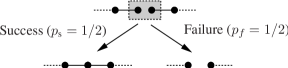
Figure 1: Action of a fusion gate on the end qubits of two linear cluster states.

III.1 Cluster states and fusion gates

A linear cluster state [12] is an instance of a graph state [13, 14] of a simple graph corresponding to a line segment. Any such graph state is associated with an undirected graph, so with $n$ vertices and a set $E$ of edges, so of pairs $(a,b)$ of connected vertices. Graph states can be defined as those states whose state vector is of the form

$$|G\rangle=\prod_{(a,b)\in E}U^{(a,b)}\left((|0\rangle+|1\rangle)/2^{1/2}\right)^{\otimes n}$$

where $U^{(a,b)}:=|0\rangle\langle 0|^{(a)}\otimes\mathbbm{1}^{(b)}+|1\rangle\langle 1|^{(a)}\otimes\sigma_{z}^{(b)}$, $\sigma_{z}$ denoting the familiar Pauli operator. In this basis, a linear cluster state vector of some length $l$ is hence just a sum of all binary words on $n$ qubits with appropriate phases. An EPR pair is consequently conceived as a linear cluster state with a single edge, $l=1$ [27]. A two-dimensional cluster state is the graph state corresponding to a two-dimensional cubic lattice. Only the describing graphs will be relevant in the sections to come; the quantum nature of graph states does not enter our considerations.

As stated before, we call a quantum mechanical gate a (type-I) fusion gate [5] if it can “fuse together” two linear cluster state “chains” with $l_{1}$ and $l_{2}$ edges respectively to yield a single chain of $l_{1}+l_{2}$ edges (see Fig. 1). The process is supposed to succeed with some probability $p_{\text{s}}$. In case of failure both chains loose one edge each: $l_{i}\mapsto l_{i}-1$. Unless stated otherwise, we will assume that $p_{\text{s}}=1/2$, in accordance with the results of the next section.

This kind of quantum gate is, yet, insufficient to build up two-dimensional cluster states. For this to be possible, another kind of fusion gate is required: type-II fusion [5] to be discussed in Section X.

III.2 Linear optical fusion gates

We use the usual convention for encoding a qubit into photons: In the so-called dual-rail encoding the basis vectors of the computational Hilbert space are represented by

$$|0\rangle := a^{\dagger}_{0}|\text{vac}\rangle$$

$$|1\rangle := a^{\dagger}_{1}|\text{vac}\rangle,$$

where $a^{\dagger}_{0,1}$ denote the creation operators in two orthogonal modes, and $|\text{vac}\rangle$ is the state vector of the vacuum. The canonical choice are two modes that only differ in the polarization degree of freedom, e. g. horizontal and vertical with respect to some reference, giving rise to the notation $|H\rangle:=|0\rangle$ and $|V\rangle:=|1\rangle$.

Type-I fusion gates were introduced in Ref. [5], where it was realized that the parity check gate [7] has exactly the desired effect. The gate’s probability of success is $p_{\text{s}}=1/2$ and the following theorem states that this cannot be increased in the setting of dual rail coded linear optical quantum computation.

Theorem 1 (Maximum probability of success of fusion).

The optimal probability of success $p_{\text{s}}$ of a type-I fusion quantum gate is $p_{\text{s}}=1/2$. More specifically, the maximal $p=p_{1}+p_{2}$ such that

$$A_{1} = p_{1}^{1/2}(|H\rangle\langle H,H|-|V\rangle\langle V,V|)/\sqrt{2},$$

$$A_{2} = p_{2}^{1/2}(|H\rangle\langle H,H|+|V\rangle\langle V,V|)/\sqrt{2}$$

are two Kraus operators of a channel that can be realized with making use of (i) any number of auxiliary modes prepared in the vacuum, (ii) linear optical networks acting on all modes, and (iii) photon counting detectors is given by $p=p_{\text{s}}:=1/2$.

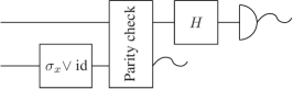
Figure 2: Diagram representing how parity check gate can be employed to realize a Bell state discriminating device.

Proof.

Given the setup in Fig. 2, we notice a parity check described by these Kraus operators can be used to realize a measurement, distinguishing with certainty two from four binary Bell states: The following Hadamard gate and measurement in the computational basis give rise to the Kraus operators

$$B_{\pm}=\langle\pm|=2^{-1/2}(\langle H|\pm\langle V|).$$

On input of the symmetric Bell states with state vectors, $|\phi^{\pm}\rangle=2^{-1/2}(|H,H\rangle\pm|V,V\rangle)$, the measurement results $(A_{1},B_{-})$ and $(A_{2},B_{+})$ indicate a $|\phi^{+}\rangle$ and $(A_{1},B_{+})$ and $(A_{2},B_{-})$ a $|\phi^{-}\rangle$, respectively. These two states can be identified with certainty. The anti-symmetric Bell states with state vectors $|\psi^{\pm}\rangle=2^{-1/2}(|H,V\rangle\pm|V,H\rangle)$, will in turn result in a failure outcome.

Applying a bit-flip (a Pauli $\sigma_{x}$) on the second input qubit (therefore implementing the map $|\phi^{\pm}\rangle\mapsto|\psi^{\pm}\rangle$, $|\psi^{\pm}\rangle\mapsto|\phi^{\pm}\rangle$) at random, a discrimination between the four Bell states with uniform a priori probabilities is possible, succeeding in 50% of all cases. Following Ref. [28] this is already the optimal success probability when only allowing for (i) auxiliary vacuum modes, (ii) networks of beam splitter and phase shifts and (iii) photon number resolving detectors. Thus, a more reliable parity check is not possible within the presented framework. ∎

In turn, it is straightforward to see that a failure necessarily leads to a loss of one edge each. Note that one could in principle use additional single-photons from sources or EPR pairs to attempt to increase the success probability $p_{\text{s}}$ of the individual gate. These additional resources would yet have to be included in the resource count. Such a generalized scenario will not be considered.

IV Concepts: Configurations and strategies

The current section will set up a rigorous framework for the description and assessment of control strategies. All considerations concern the case of one-dimensional cluster states; the two dimensional case will be deferred to Section X. Note that, having described the action of the elementary gate on the level of graphs, we may abstract from the quantum nature of the involved cluster states altogether.

IV.1 Configurations

A configuration (in the identity picture) $I$ is a list of numbers $I_{k},k\in\mathbbm{N}$. We think of $I_{k}$ as specifying the length of the $k$-th chain that is available to the experimenter at some instance of time. For most of the statements to come a more coarse-grained point of view is sufficient: in general we do not have to distinguish different chains of equal length. It is hence expedient to introduce the anonymous representation of a configuration $C$ as a list of numbers $C_{i},i\in\mathbbm{N}$ with $C_{i}$ specifying the numbers of chains of length $i$. We will always use the latter description unless stated otherwise. Trailing zeroes will be suppressed, i. e. we abbreviate $C=1,2,0,\dots$ as $C=(1,2)$. Define the total number of edges (total length) to be $L(C)=\sum_{i}i\,C_{i}$. The space of all configurations is denoted by $\mathcal{C}$. By $\mathcal{C}^{(N)}$ we mean the set of configurations $C$ having a total length less or equal to $N$. Lastly, let $e_{i}$ be the configuration consisting of exactly one chain of length $i$. This definition allows us to expand configurations as $C=\sum_{i=1}^{\infty}C_{i}\,e_{i}$.

IV.2 Elementary rule

Let us re-formulate the action of the fusion gate in this language. An attempted fusion of two chains of length $k$ and $l$ gives rise to a map $C=\sum_{i=1}^{\infty}C_{i}e_{i}\mapsto C^{\prime}=\sum_{i=1}^{\infty}C_{i}^{\prime}e_{i}$ with

$$C^{\prime}=C-e_{k}-e_{l}+e_{k+l}$$

in case of success with probability $p_{\text{s}}=1/2$ (leading to a single chain of length $l+k$) and

$$C^{\prime}=C-e_{k}+e_{k-1}-e_{l}+e_{l-1}$$

in case of failure, meaning that one edge each is lost for the chains of length $k$ and $l$. All other elements of $C$ are left unchanged.

IV.3 Strategies

A strategy (in the anonymous picture) defines what action to take when faced with a specific configuration. Actions can be either “try to fuse a chain of length $k$ with one of length $l$” or “do nothing”. Formally, we will represent these choices by the tuple $\langle k,l\rangle$ and the symbol ${\emptyset}$, respectively. It is easy to see that, in trying to build up a single long chain, it never pays off not to use all available resources. We hence require a strategy to choose a non-trivial action as long as there is more than one chain in the configuration. Formally, a strategy is said to be valid if it fulfills

1. (No null fusions): $S(C)=\langle k,l\rangle\Rightarrow C_{l},C_{k}\neq 0$

2. (No premature stops): $S(C)={\emptyset}\Leftrightarrow$ $C$ contains at most one chain.

We will implicitly assume that all strategies that appear are valid. Strategies in the identity picture are defined completely analogously.

An event $E$ is a string of elements of $\{S,F\}$, denoting success and failure, respectively. The $i$-th component of $E$ is denoted by $E_{i}$ and its length by $|E|$. Now fix an initial configuration $C_{\emptyset}$ and some strategy $S$. We write $C_{E}$ for the configuration which will be created by $S$ out of $C_{\emptyset}$ in the event $E$. Here, as in several definitions to come, the strategy $S$ is not explicitly mentioned in the notation. It is easy to see that any strategy acting on some initial configuration will, in any event, terminate after a finite number of steps $n_{\text{T}}(C)$.

Recall that the outcome of each action is probabilistic and a priori we do not know which $C_{E}$ with $|E|=n$ will have been obtained in the $n$-th step. It is therefore natural to introduce a probability distribution on $\mathcal{C}$, by setting

$$p_{n}(C):=2^{-n}\,|\{E:|E|=n,C_{E}=C\}|.$$

In words: $p_{c}(C)$ equals $2^{-n}$ times the number of events that lead to $C$ being created. The fact that $S$ terminates after a finite number of steps translates to $p_{n_{\text{T}}+k}=p_{n_{\text{T}}}$ for all positive integers $k$. Expectation values of functions $f$ on $\mathcal{C}$ now can be written as

$$\langle f\rangle_{p_{n}}:=\sum\limits_{C}p_{n}(C)f(C).$$

The expected total length is

$$\langle L\rangle_{p_{n}}:=\sum\limits_{C,i}p_{n}(C)i\,C_{i}.$$

In particular, the expected final length is given by $\tilde{Q}(C_{\emptyset}):=\langle L\rangle_{p_{n_{\text{T}}}}$. Of central importance will be the best possible expected final length that can be achieved by means of any strategy:

$$Q(C_{\emptyset}):=\sup_{S}\tilde{Q}_{S}(C_{\emptyset}).$$

This number will be called the quality of $C_{\emptyset}$. For convenience we will use the abbreviations $\tilde{Q}(N):=\tilde{Q}(Ne_{1})$ and $Q(N):=Q(Ne_{1})$.

V Simple strategies

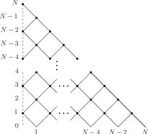
Figure 4: The process of fusion of the largest can be represented as a tree similar to a random walk. Reflection occurs at the dashed line (the largest string is lost and replaced with an EPR pair. Time evolves from top to bottom, thus decreasing the number of EPR resources. The horizontal dimension represents the length of the largest string.

A priori, a strategy does not allow for a more economic description other than a ’look-up table’, specifying what action to take when faced with a given configuration. If one restricts attention to the set of configurations $\mathcal{C}^{(N)}$ that can be reached starting from $N$ EPR pairs, $|\mathcal{C}^{(N)}|$ values have to be fixed.

The cardinality $|\mathcal{C}^{(N)}|$, in turn, can be derived from the accumulated number of integer partitions of $k\leq N$. The asymptotic behavior [29] can be identified to be

$$|\mathcal{C}^{(N)}|=\frac{1+O(N^{-1/6})}{({8\pi^{2}N})^{1/2}}\mathrm{e}^{\pi({2N}/{3})^{1/2}},$$

which is exponential in the number $N$ of initially available EPR pairs [30].

However, there are of course strategies which do allow for a simpler description in terms of basic general rules that apply similarly to all possibly configurations. It might be surmised that close-to-optimal strategies can be found among them. Also, these simple strategies are potentially accessible to analytical and numerical treatment. Subsequently, we will discuss three such reasonable strategies, referred to as Greed, Modesty, and Static.

V.1 Greed

This is one of the most intuitive strategies. It can be described as follows: “Given any configuration, try to fuse the largest two available chains”. This is nothing but

$$S_{G}(C)=\left\{\begin{array}[]{ll}\emptyset&\text{if $\sum_{i}C_{i}\leq 1$}\\ \langle k,l\rangle&\begin{array}[]{lcl}k&=&\max\{i:C_{i}>0\}\\ l&=&\max\{i:C_{i}-\delta_{i,k}>0\}\end{array}\end{array}\right..$$

Alternatively, one may think of Greed as fusing the first two chains after sorting the configuration in descending order. The rationale behind choosing this strategy is the following: fusing is a probabilistic process which destroys entanglement on average. Hence it should be advantageous to quickly build up as long a chain as possible. Clearly, the strategy’s name stems from its pursuit of short-term success. From a theoretical point of view, Greed is interesting, as its asymptotic performance can easily be assessed (see Fig. 5):

Lemma 2 (Asymptotic performance of Greed).

The expected length of the final chain after applying Greed to $N$ EPR pairs scales asymptotically as

$$\tilde{Q}_{G}(N)=({2N}/{\pi})^{1/2}+o(1).$$

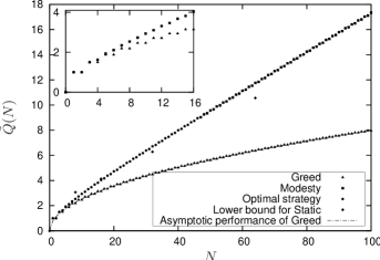
Figure 5: Expected length for the globally optimal strategy, for Modesty (in this plot indistinguishable from the former), for Greed, its asymptotic performance, and the lower bound for Static, as functions of even number $N$ of initial EPR pairs. The inset shows Greed and Modesty for small $N$, revealing the parity-induced step-like behavior.

Proof.

It is easy to see that an application of Greed to $C_{\emptyset}=Ne_{1}$ only generates configurations in $\bigl{\{}me_{1}+e_{l},m=0,\ldots,N;l=0,\ldots,N;l+m\leq N\bigr{\}}$. This set is parametrized by $m$ (the number of EPR resources) and $l$ giving rise to the notation $C=(l,m)$. By definition of $S_{G}$, whenever $l\geq 1$, the next fusion attempt is made on this longer chain and one of the other EPR pairs. As for the case $l=0$ we identify $(0,m)$ with $(1,m-1)$ (when encountering $(0,m)$ we distinguish one of the $m$ pairs). Therefore, in this slightly modified notation we have with $C_{E}=(l,m),l>0$ in case of success $C_{ES}=(l+1,m-1)$ and in case of failure $C_{EF}=(l-1,m-1)$, respectively.

The tree in Fig. 4 can be obtained by reflecting the negative half of a standard random walk tree at $l=0$ and identifying the vertices with same $m$ but opposite $l$. One can readily read off the expectation value of final chain’s length. The form is especially simple in the balanced case ($p_{\text{s}}=1/2$),

$$\tilde{Q}_{G}(N)=2\sum\limits_{k=0}^{\left\lfloor(N-1)/2\right\rfloor}p_{\text{s}}^{k}(1-p_{\text{s}})^{N-k}{N\choose k}\left(N-2k\right).$$

The probabilities are twice the probabilities of the standard random walk tree, and the length-$0$ term has been omitted.

Using an estimate using a Gaussian distribution we easily find the asymptotic behavior for large $N$ (setting $\mu=pN$ and $\sigma^{2}=p_{\text{s}}(1-p_{\text{s}})N$ with $p_{\text{s}}=1/2$),

$$\tilde{Q}_{G}(N) = \left({\frac{8}{N\pi}}\right)^{1/2}\int\limits_{0}^{\infty}2x\exp\left(-\frac{2x^{2}}{N}\right)\mathrm{d}x+r(N)$$

$$= \left(\frac{2N}{\pi}\right)^{1/2}\Gamma(1)+r(N)$$

with approximation error $r(N)=o(1)$. ∎

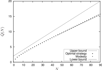
Figure 6: Expected length for Modesty, the optimal strategy (where known) a lower bound to the quality as in Theorem 6, but with $N_{0}=46$ (for better visualization), and the upper bound attained with the razor model as functions of the number of initial EPR pairs $N$.

The behavior of Greed changes qualitatively upon variation of $p_{\text{s}}$: For $p_{\text{s}}>1/2$, $\tilde{Q}_{G}(N)$ shows linear asymptotics in $N$, while in case of $p_{\text{s}}<1/2$ the quality $\tilde{Q}_{G}(N)$ is not even unbounded as a function of $N$.

There is a phenomenon present in the performance of many strategies, which can be understood particularly easily when considering Greed: $\tilde{Q}$ displays a “smooth” behavior when regarded as a function on either only even or only odd values of $N$. However, the respective graphs appear to be slightly displaced with respect to each other. For simplicity, we will in general restrict our attention to even values and explore the reasons for this behavior in the following lemma.

Lemma 3 (Parity and $\tilde{Q}_{G}$).

Let $N$ be even. Then $\tilde{Q}_{G}(N)=\tilde{Q}_{G}(N+1)$.

Proof.

Let $C_{\emptyset}=Ne_{1},C^{\prime}_{\emptyset}=(N+1)e_{1}$, for $N$ even. Now let $E$ be such that $S(C_{E})={\emptyset}$ but $S(C_{E_{1,\ldots,|E|-1}})\neq{\emptyset}$. As Greed does not touch the $i$-th chain before the $i$-th step, it holds that $C^{\prime}_{E}=C_{E}+e_{1}$. Further, since type-I fusion preserves the parity of the total number of edges, $C^{\prime}_{E}\neq 0$. Hence $C^{\prime}_{E}$ is of the form $C^{\prime}_{E}=e_{1}+e_{k}$ and one computes:

$$\tilde{Q}_{G}(C^{\prime}_{E}) = 1/2(k+1)+1/2(k-1)=k=\tilde{Q}_{G}(C_{E}).$$

From here, the assertion is easily established by re-writing $\tilde{Q}_{G}(C^{\prime}_{\emptyset})$ as a suitable average over terms of the form $Q_{G}(C^{\prime}_{E})$, where $E$ fulfills the assumptions made above. ∎

As a corollary to the above proof, note that fusing an EPR pair to another chain does not, on average, increase its length. Hence the fact that $\tilde{Q}_{G}(N)$ grows at all as a function of $N$ is solely due to the asymmetric situation at length zero.

Lemma 3 explains the steps apparent in Fig. 5. Such steps are present also in the performance of Modesty, to be discussed now, and several other strategies – albeit not in such a distinct manner.

V.2 Modesty

There is a very natural alternative to the previously studied strategy. Instead of trying to fuse always the largest existing linear cluster states in a configuration, one could try the opposite: “Given any configuration, try to fuse the smallest two available chains”. In contrast to Greed this strategy intends to build up chains of intermediate length, making use of the whole EPR reservoir before trying to generate larger chains. Even though no long chains will be available at early stages, the strategy might nevertheless perform reasonably. Quite naturally, this strategy we will call Modesty.

Formally, this amounts to replacing $\max$ by $\min$, i. e. replacing descending order by ascending order:

$$S_{M}(C)=\left\{\begin{array}[]{ll}\emptyset&\text{if $\sum_{i}C_{i}\leq 1$}\\ \langle k,l\rangle&\begin{array}[]{lcl}k&=&\min\{i:C_{i}>0\}\\ l&=&\min\{i:C_{i}-\delta_{i,k}>0\}\end{array}\end{array}\right..$$

Maybe surprisingly, Modesty will not only turn out to give better results than Greed, but is actually close to being globally optimal, as can be seen in Figures 5 and 6. See Section VI.2 for a closer discussion.

V.3 Static

Another strategy of particular interest is called Static, $S_{S}$. To describe its action, we need to define the notion of an insistent strategy. The term is only meaningful in the identity picture, which we will employ for the course of this section. Now, a strategy is called insistent if, whenever it decides to fuse two specific chains, it will keep on trying to glue these two together until either successful or at least one of the chains is completely destroyed. Formally:

$$S(C_{E})=\langle k,l\rangle\wedge(C_{EF})_{k}(C_{EF})_{l}\neq 0\Rightarrow S(C_{EF})=S(C_{E})$$

Static acts by insistingly fuse the first chain to the second one; the third to the fourth and so on. After this first level, the resulting chains will be renumbered in the way that the outcome of the $k$-th pair is now the $k$-th chain. At this point, Static starts over again, using the configuration just obtained as the new input. This procedure is iterated until at most one chain of nonzero length has survived.

The proceeding of $S_{S}$ is somehow related to Modesty and Greed, just without sorting the chains between fusion attempts. This results in much less requirements on the routing of the photons actually carrying the cluster states. From an experimentalist’s point of view, Static is a meaningful choice as it only requires a minimal amount of classical feed-forward that is only present at the level of fusion gates, not on the level of routing the chains. It performs, however, asymptotically already better than Greed (see Fig. 5).

It turns out that Static performes rather poorly when acting on a configuration consisting only of EPR pairs. To cure this deficit, we will proceed in two stages. Firstly, the input is partitioned into blocks of eight EPR pairs each. Then Modesty is used to transform each block into a single chain. The results of this first stage are subsequently used as the input to Static proper, as described before. Slightly overloading the term, we will call this combined strategy Static as well. Note that, even when understood in this wider sense, Static still reduces the need for physically re-routing chains: the blocks can be chosen to consist of neighboring qubits and no fusion processes between chains of different blocks are necessary during the first stage. The following theorem bounds Static’s performance. For technical reasons, it is stated only for suitable $N$.

Theorem 4 (Linear performance of Static).

For any $m\in\mathbbm{N}$, given $N=2^{3+m}$ EPR pairs, Static will produce a single chain of expected length

$$\tilde{Q}(N)\geq(137/1024)N+2.$$

The proof of the above theorem utilizes the following lemma which quantifies the quality one expects when combining several configurations.

Lemma 5 (Combined configurations).

The following holds.

1. Let $C$ be a configuration consisting of single chains of respective length $l_{1},l_{2}$. Then [31]

   $$Q(C)=l_{1}+l_{2}-2+2^{1-\min(l_{1},l_{2})}\geq l_{1}+l_{2}-2.$$ (1)

2. Let $C_{(1)},\dots,C_{(k)}$ be configurations. Let $S$ be a strategy that acts on $\sum_{i}C_{(i)}$ by first acting with $S^{\prime}$ on each of the $C_{(i)}$ and then acting insistently on the resulting chains. Then [32],

   $$\tilde{Q}_{S}\left(\sum_{i}C_{(i)}\right)\geq\sum_{i}\tilde{Q}_{S^{\prime}}(C_{(i)})-2(k-1).$$

3. When substituting all occurences of $\tilde{Q}$ by $Q$, the above estimate remains valid.

Proof.

Firstly, any strategy will try to fuse the only two chains in the configuration together until it either succeeds or the shorter one of the two is destroyed (after $\min(l_{1},l_{2})$ unsuccessful attempts). In other word: in case of these special configurations any strategy is insistent. By Lemma 7:

$$Q(l_{1},l_{2}) = l_{1}+l_{2}-\langle T\rangle$$

$$= l_{1}+l_{2}-\sum_{i=0}^{\min(l_{1},l_{2})-1}2^{-i}$$

$$= l_{1}+l_{2}-2+2^{1-\min(l_{1},l_{2})}.$$

For the second part, we run $S^{\prime}$ on each $C_{(i)}$, resulting in $k$ single chain configurations $C^{\prime}_{(i)}=e_{l_{i}}$ with probability distributions $p_{i}$ on $\mathcal{C}$ obeying $\tilde{Q}_{S^{\prime}}(C^{\prime}_{(i)})=\langle l_{i}\rangle_{p_{i}}$. The joint distribution on $\mathcal{C}^{k}$ is given by $p=\prod_{i}p_{i}$. Now we fuse the chains together. If $C^{\prime}_{(i)}$ and $C^{\prime}_{(j)}$ are such that $p_{i}(C^{\prime}_{(i)})p_{j}(C_{(j)})\neq 0$, we unite them into one configuration $C:=C_{(i)}+C_{(j)}$. Clearly, $C$ contains at most two chains which we fuse together as described in the first part of the Lemma. As Eq. (1) is linear in the respective lengths of the chains in $C$, the distribution $p^{\prime}=p_{i}p_{j}$ fulfills on the one hand

$$\langle\tilde{Q}\rangle_{p^{\prime}}=\langle L\rangle_{p^{\prime}}\geq\langle L\rangle_{p_{i}}+\langle L\rangle_{p_{j}}-2$$

and on the other hand

$$\tilde{Q}((\langle l_{i}\rangle_{p_{i}},\langle l_{j}\rangle_{p_{j}}))\geq\langle L\rangle_{p_{i}}+\langle L\rangle_{p_{j}}-2.$$

for any insistent strategy. Because these two quantities are bounded by the same value we will use this bound and replace averages over $\tilde{Q}$ with $\tilde{Q}$ of configurations of average lengths.

We now iterate this scheme to obtain a single chain. A moment of thought reveals that – as a result of our neglecting the $2^{1-\min(l_{1},l_{2})}$-term – the order in which chains are fused together does not enter the estimate for $\tilde{Q}_{S}$. The claim follows.

As for the third point: It follows by setting $S^{\prime}$ to the optimal strategy. ∎

Proof.

(of Theorem 4) Consider a configuration consisting of $n=2^{m}$ chains of length $x$ each. Using Lemma 5 one sees that the second stage of Static will convert it into a single chain of expected length $\tilde{Q}(2^{m}e_{x})\geq(x-2)n+2$.

According to Section VI, Modesty fulfils $\tilde{Q}_{M}(8)=Q(8)=649/256$. Applying Lemma 5 again we find with $x=\tilde{Q}_{M}(2^{3})$ and $N=2^{3+m}$

$$\tilde{Q}_{S}(N) \geq \frac{649/256-2}{8}N+2=\frac{137}{2048}N+2$$

$$\approx 6.69\ 10^{-2}N+2.$$

∎

In case of $p_{\text{s}}\neq 1/2$,

$$\tilde{Q}^{\prime}_{S}(ne_{x})\geq n(x-l_{\text{initial}})+l_{\text{initial}}$$

can be obtained in the same way, where $l_{\text{initial}}=2(1-p_{\text{s}})/p_{\text{s}}$ (similar to $n_{c}$ in [19]). Initial chains of length $\geq l_{\text{initial}}$ can be produced by employing for example Greed, but disregarding the outcome in case of a fusion failure and aborting the process when $2(1-p_{\text{s}})/p_{\text{s}}$ is reached. Although large chains are produced with only a small overall success probability, this does not effect the linear asymptotics as this process only depends on $p_{\text{s}}$, rather than $N$.

VI Computer-assisted results

VI.1 Algorithm for finding the optimal strategy

Before passing from the concrete examples considered so far to the more abstract results of the next sections, it would be instructive to explicitly construct an optimal strategy for small $N$. Is that a feasible task for a desktop computer? Naively, one might expect it not to be. Since the number of strategies grows super-exponentially as a function of the total number of edges $N$ of the initial configuration, a direct comparison of the strategies’ performances is quickly out of reach. Fortunately, a somewhat smarter, recursive algorithm can be derived which will be described in the following paragraph.

The number of vertices in a configuration is given by $V(C):=\sum_{i}C_{i}(n_{i}+1)$. An attempted fusion will decrease $V(C)$ regardless of whether it succeeds or not. Now fix a $V_{0}$ and assume that we know the value of $Q$ for all configurations comprised of up to $V_{0}$ vertices. Let $C$ be such that $V(C)=V_{0}+1$. It is immediate that

$$Q(C)=\text{max}_{i,j}\,(Q(\text{S}_{i,j}\,C)+Q(\text{F}_{i,j}\,C))/2,$$

where $\text{S}_{i,j}\,C$ denotes the configuration resulting from successfully fusing chains of lengths $l_{i}$ and $l_{j}$. $\text{F}_{i,j}C$ is defined likewise. As the r. .h. s. involves only the quality of configurations possessing less than or equal to $V_{0}$ vertices, we know its value by assumption and we can hence perform the maximization in $O(c^{2})$ steps. One thus obtains the quality of $C$ and the pair of chains that need to be fused by an optimal strategy.

The algorithm now works by building a lookup table containing the value of $Q$ for all configurations up to a specific $V_{\text{max}}$. It starts assessing the set of configurations with $V(C)=1$ and works its way up, making at each step use of the previously found values. One needs to supply an anchor for the recursion by setting $Q(e_{i})=i$. Clearly, the memory consumption is proportional to $|{\cal C}^{(N)}|$, which is exponential in $N$ and will limit the practical applicability of the algorithm before time issues do.

We have implemented this algorithm using the computer algebra system Mathematica and employed it to derive in closed form an optimal strategy for all configurations in ${\cal C}^{(46)}$, the quality of which is shown in Figures 5 and 6. A desktop computer is capable of performing the derivation in a few hours [33].

From the discussion above, it is clear that the leading term in the computational complexity of the algorithm is given by $|C^{(N)}|$: every configuration needs to be looked at at least once. A straight-forward analysis reveals a poly-log correction; the described program terminates after $O\big{(}|C^{(N)}|\,(\log|C^{(N)}|)^{5}\big{)}$ steps.

VI.2 Data, intuitive interpretation, and competing tendencies

Starting with $C_{\emptyset}=Ne_{1}$, Modesty turns out to be the optimal strategy for $N\leq 10$. For configurations containing more edges, slight deviations from Modesty can be advantageous. The difference relative to $Q(N)$ is smaller than $1.1\times 10^{-3}$ for $N\leq 46$. More generally, two heuristic rules seem to hold:

1. It is favorable to fuse small chains (this is the dominant rule).

2. It is favorable to create chains of equal length.

Is there an intuitive model which can explain these findings? Several steps are required to find one. Firstly, note that every fusion attempt entails a $1/2$ probability of failure, in which case two edges are destroyed. So “on average” the total length $L(C)$ decreases by one in each step and it is natural to assume that the quality $Q(C)$ equals $L(C)$ minus the expected number of fusion attempts a specific strategy will employ acting on $C$. Hence a good strategy aims to reach a single-chain configuration as quickly as possible, so as to reduce the expected number of fusions (this reasoning will be made precise in Section VIII). Now, if there are $k$ chains present in $C$, then a priori $k-1$ successful fusions are needed before a strategy can terminate. If, however, in the course of the process one chain is completely destroyed, then $k-2$ successes would already be sufficient. Therefore – paradoxically – within the given framework it pays off to destroy chains. Since shorter chains are more likely to become completely consumed due to failures, they should be subject to fusion attempts whenever possible. This explains the first rule.

There is one single scenario in which two chains can be destroyed in a single step; that is when one selects two EPR pairs to be fused together. Now consider the case where there are two chains of equal length in a configuration. If we keep on trying to fuse these two chains, then – in the event of repeated failures – we will eventually be left with two EPR pairs, which are favorable to obtain as argued before. Hence the second rule.

We have thereby identified two competing tendencies of the optimal strategy. Obtaining a quantitative understanding of their interplay seems extremely difficult: deviating from Modesty at some point of time might open up the possibility of creating two chains of equal lengths many steps down the line. We hence feel it is sensible to conjecture that the globally optimal strategy allows not even for a tractable closed description. A proof of its optimality seems therefore beyond any reasonable effort. One is left with the hope of obtaining appropriately tight analytical bounds – and indeed, the sections to come pursue this programme with perhaps surprising success.

VII Lower bound

We will now turn to establishing rigorous upper and lower bounds to $Q$, so the quality of the optimal strategy. These bounds, in turn, give rise to bounds to the resource consumption any linear optical scheme will have to face. Lower bounds are in turn less technically involved than upper bounds. In fact, rigorous lower bounds can be based on known bounds for given strategies: For not too-large configurations, the performance of various strategies can be calculated explicitly on a computer (see Section VI). Any such computation in turn gives a lower bound to $Q$. The following theorem is based on a construction which utilizes the computer results to build a strategy valid for inputs of arbitrary size. This strategy is simple enough to allow for an analytic analysis of its performance while at the same time being sufficiently sophisticated to yield a very tight lower bound for the quality, shown in Fig. 6. Notably, the resulting statement is not a numerical estimate valid for small $N$, but a proven bound valid for all $N$:

Theorem 6 (Lower bound for globally optimal strategy).

Starting with $N$ EPR pairs and using fusion gates, the globally optimal strategy yields a cluster state of expected length

$$Q(N)\geq\tilde{Q}(N_{0})+\alpha(N-N_{0}),$$ (2)

for all $N\geq N_{0}$. The constants are

$$N_{0} = 92,\qquad\tilde{Q}(N_{0})=16.1069,$$

$$\alpha = (\tilde{Q}(N_{0})-2)/N_{0}=0.153336.$$

Rational expression are known and can be accessed at Ref. [33].

Proof.

Denote by $\tilde{Q}(N)$ the expected final length of some strategy acting on $N$ EPR pairs. Fix $N_{0}$ such that $\tilde{Q}(N)$ is known for all $N\leq 2N_{0}$ and $\tilde{Q}$ satisfies for $N_{0}\leq N\leq 2N_{0}$

$$(\tilde{Q}(N)-2)/{N}\geq(\tilde{Q}(N_{0})-2)/N_{0}$$ (3)

and that Eqn. (2) holds for all $N\leq 2N_{0}$.

Now assume we are given $N>2N_{0}$ EPR pairs. Clearly, there are positive integers $k\geq 2$ and $M\leq N_{0}$ such that $N=kN_{0}+M$. Set $n_{i}=N_{0}$ for $i=1,\dots,k-1$ and $n_{k}=N_{0}+M$. The $n_{i}$ fulfill $\sum_{i}n_{i}=N$ and $N_{0}\leq n_{i}\leq 2N_{0}$. We partition the input into blocks of length $n_{i}$ each and compute

$$Q\left(\sum_{i}n_{i}\right) \geq \sum_{i=1}^{k}Q(n_{i})-2(k-1)$$

$$\geq \sum_{i=1}^{k}\tilde{Q}(n_{i})-2(k-1)$$

$$= \tilde{Q}(N_{0})+\sum_{i=2}^{k}n_{i}\frac{\tilde{Q}(n_{i})-2}{n_{i}}$$

$$\geq \tilde{Q}(N_{0})+\sum_{i=2}^{k}n_{i}\frac{\tilde{Q}(N_{0})-2}{N_{0}}$$

$$= \tilde{Q}(N_{0})+\alpha\sum_{i=2}^{k}n_{i}$$

$$= \tilde{Q}(N_{0})+\alpha(N-N_{0}),$$

where we made use of Lemma 5 and the assumptions mentioned above.

In the case of Modesty the function $\tilde{Q}_{M}(N)$ can be explicitly computed for not too large values of $N$. Indeed, the results for all $N\leq 2N_{0}=184$ can be found at [33]. They obey the condition in Eqn. (3) and the statement follows with $\tilde{Q}_{M}(N_{0})=16.1069$. ∎

VIII Upper bounds

While the performance of any strategy delivers a lower bound for the optimal one, giving an upper bound is considerably harder. We will tackle the problem by passing to a family of simplified models. For every integer $R\geq 2$, the razor model with parameter $R$ is defined by introducing the following new rule: after every fusion step all chains will be cut down to a maximum length of $R$. Obviously, the full problem may be recovered with $R\geq N$. Given the complexity of the problem, it comes as a surprise that even for parameters as small as $R=2$ the essential features of the full setup seem to be retained by the simplification, in the sense that understanding the razor model yields extraordinary good bounds for $Q$.

VIII.1 The razor model – outline

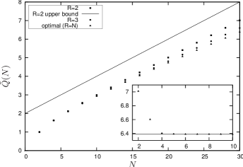
Figure 7: Performance of the optimal strategy in the razor model ($R=2$ and $R=3$), the full model ($R=N$) and the upper bound attained with the $R=2$ razor model. The inset shows the convergence of the upper bound to the quality (based on the razor model with parameter $R$) vs. the razor parameter $R=2,\ldots,10$ for $N=30$ together with the optimal value $Q(30)$.

In the spirit of Section IV, a configuration in the razor model is specified by a vector in $\mathbbm{N}^{R}$. Thus, the number of configurations with a maximum total number of $N$ edges is certainly smaller than $N^{R}$, which is a polynomial in $N$. Adapting the techniques presented in Section VI, we can obtain the optimal strategy with polynomially scaling effort. We have thus identified a family of simplified problems which, in the limit of large $R$, tend to become exact, and where each instance is solvable in polynomial time.

How do the results of the razor model relate to the original problem? Clearly, for small values of $R$, $Q_{\text{razor}}(C)$ will be a very crude lower bound to $Q(C)$. However, as indicated in Section VI, the quality of a configuration $C$ can be assessed in terms of the optimal strategy’s expected number of fusion attempts $\langle T(C)\rangle$ when acting on $C$. It is intuitive to assume that $\langle T\rangle\leq\langle T\rangle_{\text{razor}}$, as the “cutting process” increases the probability of early termination. We will thus employ the following argument: for a given configuration $C$, derive a lower bound for $\langle T(C)\rangle_{\text{razor}}$, which is in particular a lower bound for $\langle T(C)\rangle$, which in turn gives rise to the upper bound

$$Q(C)\leq L(C)-\langle T(C)\rangle$$

for $Q$.

The results of this ansatz are extremely satisfactory. Fig. 7 shows the performance of the optimal quality for various $R$, and the convergence when increasing $R$.

The intuitive explanation for the success of the model is the observation that the chance that a chain of length $R$ is built up, and eventually again disappears, is exponentially suppressed as a function of $R$. That is, the crucial observation is that the error made by this radical modification is surprisingly small. A rigorous justification for this reasoning is supplied by the following two propositions which will be proved in the next section.

Lemma 7 (Quality and attemped fusions).

The expected final length $\langle L\rangle$ equals the initial number of edges $L(C_{\emptyset})$ minus the expected number of attempted fusions $\langle T\rangle$.

Theorem 8 (Bound to the full model from the razor model).

Let $C_{\emptyset}\in\mathcal{C}$ be a configuration. The optimal strategy in the setting of the razor model will use fewer fusion attempts on average to reach a final configuration starting from $C_{\emptyset}$ than will the optimal strategy of the full setup.

VIII.2 The razor model – proofs

For the present section, it will prove advantageous to introduce some alternative points of view on the concepts used so far. Recall that a strategy is a function from configurations to actions. However, once we have fixed some initial configuration $C_{\emptyset}$, we can alternatively specify a strategy as a map from events to actions. Indeed, the configuration present after $n$ steps is completely fixed by the knowledge of the initial configuration, the past decisions of the strategy and the succession of failures and successes. We will call the resulting mapping the decision function $D_{S,C_{\emptyset}}$ and will suppress the indices whenever no danger of confusion can arise. In the same spirit, we are free to conceive random variables on $\mathcal{C}$ as real functions $f:\{S,F\}^{n}\to\mathbbm{R}$. Expectation values are then computed as

$$\langle f\rangle:=\langle f\rangle(p_{n_{\text{T}}})\sum_{E,|E|=n_{\text{T}}}2^{-|E|}f(E).$$

Quantities of the form $\langle f\rangle(C)$ for some configuration $C$ refer expectation values $\langle f\rangle$ given the initial configuration $C_{\emptyset}=C$.

An interesting class of random variables can be written in the form

$$f(E)=\sum_{i=1}^{|E|}\phi_{f}(E_{1,\dots,i})$$ (4)

where $\phi_{f}$ is some function of events and $E_{1,\dots,i}$ denotes the restriction of $E$ to its first $i$ elements. A simple example is the amount of lost edges $M(E)$ that was suffered as a result of $E$. Here,

$$\phi_{M}(E_{1,\dots,i})=\left\{\begin{array}[]{ll}2,&E_{i}=F\wedge D(E_{1,\dots,i-1})\neq{\emptyset},\\ 0,&\text{else}.\end{array}\right.$$ (5)

Let us refer to observables as in Eq. (4) as additive random variables. The following lemma states that when evaluating expectation values of additive variables, only their step-wise mean

$$\bar{\phi}(E_{1\dots i}):=\big{(}\phi(E_{1,\dots,i-1},S)+\phi(E_{1,\dots,i-1},F)\big{)}/2$$

enters the calculation.

Lemma 9 (Expectation values of additive random variables).

Let $f$ be an additive random variable. Set

$$\bar{f}(E):=\sum_{i=1}^{|E|}\bar{\phi}(E_{1\dots i}).$$

Then $\langle f\rangle=\langle\bar{f}\rangle$.

Proof.

Set $n=n_{\text{T}}$. We then have, by definition,

$$\langle f\rangle = 2^{-n}\sum_{E,|E|=n}\sum_{i=1}^{n}\phi(E_{1,\dots,i})$$

$$= \sum_{i=1}^{n}2^{-i}\sum_{E,|E|=i}\phi(E)$$

$$= \sum_{i=1}^{n}2^{-i}\sum_{E,|E|=i}\bar{\phi}(E)=\langle\bar{f}\rangle.$$

∎

Note that

$$\bar{\phi}_{M}(E_{1,\dots,i})=\left\{\begin{array}[]{ll}1,&D(E_{1,\dots,i-1})\neq{\emptyset},\\ 0,&\text{else},\end{array}\right.$$

in other words, $\bar{\phi}_{M}$ counts the number of attempted fusions $T$. Using Lemma 9, we see that the expected number of lost edges equals the expected number of fusion attempts: $\langle M\rangle=\langle T\rangle$. This proves Lemma 7.

In the following proof of Theorem 8, we will employ the identity picture introduced in Section IV. The argument is broken down into a series of lemmas.

Lemma 10 (More is better than less).

Let $I$ be a configuration. Then, for all $i$, $Q(I+e_{i})\geq Q(I)$.

Proof.

The proof is by induction on two parameters: on the number of chains $|C|$ and on the total length $L(C)$. To base the induction in both variables, we note that the claim is trivial if either $|C|\leq 1$ or $L\leq 2$.

Now consider any configuration $C$. Let $S$ be the optimal strategy and denote by $C_{S}$ and $C_{F}$ the configurations created by $S(C)$ in case of success and failure respectively. It is simple to check that $S(C)$ acting on $C+e_{i}$ yields $C_{S}+e_{i}$ or $C_{F}+e_{i}$. Hence

$$Q(C+e_{i}) \geq 1/2\big{(}Q(C_{S}+e_{i})+Q(C_{F}+e_{i})\big{)}.$$

But unless $|C|\leq 1$ we have that in any event $E\in\{S,F\}$ either $|C_{E}|<|C|$ or $L(C_{E})<L(C)$ and thus the claim follows by induction. ∎

Lemma 11 (Winning is better than losing).

Let $C\in\mathcal{C}$, let $C_{S}$ be the configuration resulting from the action of the optimal strategy on $C$ in the case of success, let $C_{F}$ be the obvious analogue. Then $Q(C_{S})\geq Q(C_{F})$.

Proof.

Let $\langle k,l\rangle$ be the action defined above. Clearly, $C_{F}=C-e_{k}-e_{l}$. By the last lemma, $Q(C_{F})\leq Q(C)$. But $Q(C)$ is the average of $Q(C_{F})$ and $Q(C_{S})$; hence

$$Q(C_{S})\geq Q(C)\geq Q(C_{F}).$$

∎

Lemma 12 (No catalysis).

Let $C\in\mathcal{C}$. Then, for all $i$, $Q(C+e_{i})\leq Q(C)+1$.

Proof.

We show the equivalent statement: for $C$ and $i$ s. t. $C_{i}\neq 0$ it holds that $Q(C-e_{i})\geq Q(C)-1$. Once more, the proof is by induction on $|C|,L$ and the validity of the claim for $|C|\leq 1$ or $L\leq 2$ is readily verified.

Let $C,S,C_{S},C_{F}$ be as in the proof of Lemma 10. If the application of $S(C)$ and the subtraction of $e_{i}$ commute, we can proceed as we did in Lemma 10. A moment of thought reveals that this is always the case if not $C_{i}=1$ and $S(C)=\langle i,k\rangle$ (or, equivalently, $\langle k,i\rangle$) for some $k$. In fact, in this case we have

$$C_{S} = (\dots,l_{i}+l_{k},\dots)$$

$$C_{F} = (\dots,l_{i}-1,\dots,l_{k}-1,\dots),$$

so that $C_{F}-e_{i}$ would take on a negative value at the $i$-th position. Note, however, that $C-e_{i}=C_{S}-e_{i}$. By induction it holds that $Q(C_{S}-e_{i})\geq Q(C_{S})-1$ and further, by Lemma 11, $Q(C_{S})-1\geq Q(C)-1$ which concludes the proof. ∎

Lemma 13 (Fewer edges – fewer fusions).

Let $C\in\mathcal{C},i$ be such that $C_{i}\neq 0$. Then

$$\langle T\rangle(C-e_{i})\leq\langle T\rangle(C),$$

where the expectation values are taken with respect to the respective optimal strategies.

Proof.

We will show that, for every $C\in\mathcal{C}$, the optimal strategy acting on $C^{\prime}:=C-e_{i}$ will content itself with a lower number of average fusion attempts $\langle T\rangle(C^{\prime})$ than will the optimal strategy acting on $C$. Recall that Lemma 7 states

$$Q(C) = L(C)-\langle T\rangle(C).$$

Combining this and Lemma 12 we find

$$Q(C^{\prime})\geq Q(C)-1$$

$$\Leftrightarrow L(C)-1-\langle T\rangle(C^{\prime})\geq L(C)-\langle T\rangle(C)-1$$

$$\Leftrightarrow \langle T\rangle(C^{\prime})\leq\langle T\rangle(C).$$

∎

We are finally in a position to tackle the original problem.

Proof.

(of Theorem 8) Let $C_{\emptyset}$ be some configuration. We will build a strategy which is valid on $C_{\emptyset}$ in the razor model and uses a fewer number of expected fusions than the optimal strategy in the full setup. Define the shaving operator $\hat{R}:\mathcal{C}\to\mathcal{C}$ which sets the length of each chain of length $i$ in the configuration it acts on to $\max(i,R)$. By a repeated application of the relation stated in Lemma 13, we see that $\langle T\rangle(\hat{R}C)\leq\langle T\rangle(C)$.

We build the razor model strategy’s decision function $D^{\prime}$ inductively for all events in $\mathcal{E}_{i}$, for increasing $i$. Consider an event $E\in\mathcal{E}_{i}$. Denote by $C^{\prime}_{E}$ the configuration resulting from $C_{\emptyset}$ under the action of $D^{\prime}$ in the event of $E$. $C^{\prime}_{E}$ is well-defined as only the values of $D^{\prime}$ for events with length smaller than $i$ enter its definition. Set $D^{\prime}(E)$ to the action taken by the optimal strategy for $\hat{R}C_{E}^{\prime}$.

It is simple to verify that $D^{\prime}$ defines a valid strategy for the razor model. By the results of the first paragraph, the expected number of fusions decreased in every step of the construction of $D^{\prime}$. The claim follows. ∎

VIII.3 An analytical bound – random walk

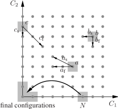
Figure 8: The configuration space of the $R=2$ razor model is $\mathbbm{N}_{0}\times\mathbbm{N}_{0}$. Only the three actions $a$, $b$ and $c$ are available to reach the final configurations (exactly one EPR pair or GHZ state, or no chain at all), starting from the initial configuration that consists of $N$ EPR pairs.

Finally, we are in a position to prove an analytic upper bound on the yield of any strategy building one-dimensional cluster chains. Quite surprisingly, the description given by the razor model with a rather radical parameter of $R=2$ is still faithful enough to deliver a good bound as will be explained now.

In the $R=2$-model configurations are fully specified by giving the number of EPR pairs $n_{1}$ and of chains of length two $n_{2}$ they contain. Hence the configuration space is $\mathbbm{N}_{0}\times\mathbbm{N}_{0}$ and we can picture it as the positive quadrant of a two-dimensional lattice. In each step a strategy can choose only among three non-trivial actions:

1. Try to fuse two EPR pairs. We call this action $a$ for brevity. Let $C_{S}$ be the configuration resulting from a successful application of $a$ on $C$. Define the vector $a_{S}\in\mathbbm{Z}\times\mathbbm{Z}$ as $a_{S}:=C_{S}-C$. An analogous definition for $a_{F}$ and some seconds of thought yield

   $$a_{S} := (-2,1),$$

   $$a_{F} := (-2,0).$$

2. Try to fuse two chains of length one and two, respectively. In the same manner as above we have

   $$b_{S} := (-1,0),$$

   $$b_{F} := (0,-1).$$

3. Try to fuse two chains of length two.

   $$c_{S} := (0,-1),$$

   $$c_{F} := (2,-2).$$

The objective is to bound from below the minimum number of non-trivial actions taken on average. Initially, we start with $N$ EPR pairs, so $C_{\emptyset}=(N,0)$. As configuration space is a subspace of $\mathbbm{N}_{0}\times\mathbbm{N}_{0}$, we can describe the situation by a random walk in a plane.

Any strategy will apply the rules $a,b,c$ until one of the points $(0,0),(1,0),(0,1)$ is reached (illustrated in Fig. 8). Our proof will be lead by the following idea: by applying one of the three non-trivial actions to a configuration $C$, we will move “on average” by

$$\bar{a} := (a_{S}+a_{F})/2=(-2,1/2),$$

$$\bar{b} := (-1/2,-1/2)\quad\text{or}$$

$$\bar{c} := (1,-3/2),$$

respectively. The minimum number of expected fusion steps should then be given by the minimum number of vectors from $\{\bar{a},\bar{b},\bar{c}\}$ one has to combine to reach the origin starting from $(N,0)$. This procedure amounts to an interchange of two averages. The aim is to reach the origin or a point with distance one to it on average as quickly as possible.

To make this intuition precise, set

$$\phi_{\delta}(E_{1,\dots,i}):=D(E_{1,\dots,i-1})_{E_{i}}.$$

Recall that $D(E_{1,\dots,i-1})$ is one of $\{a,b,c,{\emptyset}\}$. Given the event $E$, $\phi_{\delta}(E)$ is the last action applied to the configuration. For any event $E=\{S,F\}^{n}$ we require that

$$\delta(E):=\sum_{i}\phi_{\delta}(E_{1,\dots,i})\leq(-N+1,1),$$ (6)

which implies in particular that the same bound holds for $\langle\delta\rangle$. Define $a(E)$ to be the number of times the strategy will have decided to apply rule “a” in the chain of events $\{E_{1,\dots,i}\,|\,i=1,\dots,|E|\}$ leading up to $E$. Formally

$$\phi_{a}(E_{1,\dots,i})=\left\{\begin{array}[]{ll}1,&D(E_{1,\dots,i-1})=a,\\ 0,&\text{else},\end{array}\right.$$

and $a(E)=\sum_{i=1}^{|E|}\phi_{a}(E_{1,\dots,i})$. Further,

$$\bar{\phi}_{\delta}(E_{1,\dots,i})=\phi_{a}(E_{1,\dots,i})\bar{a}+\dots+\phi_{c}(E_{1,\dots,i})\bar{c},$$

where $\phi_{b},\phi_{c}$ are defined in the obvious way. It follows that

$$\langle\delta\rangle = \langle\bar{\delta}\rangle=\langle a\rangle\bar{a}+\langle b\rangle\bar{b}+\langle c\rangle\bar{c}\leq(-N+1,1),$$ (7)

$$\langle T\rangle = \langle a\rangle+\langle b\rangle+\langle c\rangle.$$ (8)

VIII.4 An analytical bound – convex optimization program

Therefore, if $\langle T\rangle$ originates from a valid strategy it is necessarily subject to the constraints put forward in Eqs. (7,8). For each $N\in\mathbbm{N}$, a lower bound for the minimum expected number of losses is thus given by a linear program, so a certain convex optimization problem: We define

$$B:=\left[\begin{array}[]{cc}-2&1/2\\ -1/2&-1/2\\ 1&-3/2\\ \end{array}\right].$$

Then, this lower bounds can be derived from the optimal solution of the linear program given by

minimize $$(1,1,1)x^{T}$$

subject to $$xB\leq(-N+1,1),$$

$$x\geq 0,$$

where the latter inequality is meant as a component-wise positivity. This is a minimization over a vector $x\in\mathbbm{R}^{3}$. In this way, the performance of the razor model is reduced to solving a family of convex optimization problems. According to Lemma 14, the solution of this linear program delivers the optimal objective value satisfying

$$\langle T\rangle=4N/5-2$$

for $N\geq 6$.

Lemma 14 (Duality for linear program).

The optimal objective values of the family of linear programs

minimize $$(1,1,1)x^{T}$$

subject to $$xB\leq(-N+1,1),$$

$$x\geq 0,$$

are given by

$$(1,1,1)x^{T}_{\text{opt}}=\left\{\begin{array}[]{ll}0,&N=1,\\ (N-1)/2,&N=2,...,5,\\ (4(N-1)-6)/5,&N\geq 6.\end{array}\right.$$

Proof.

This can be shown making use of Lagrange duality for linear programs. The dual to the above problem, referred to as primal problem, is found to be

maximize $$(N-1,-1)y^{T}$$

subject to $$-yB^{T}\leq(1,1,1),$$

$$y\geq 0.$$

This is a maximization problem in $y\in\mathbbm{R}^{2}$, again a linear program (moreover, a duality gap can never appear, i. e., the objective values of the optimal solutions of the primal and the dual problems are identical). By finding – for each $N$ – a solution of the dual problem, which is assumed by the primal problem, we have hence proven optimality of the respective solution. For all $N$, this family of solutions can be determined to be

$$y=\left\{\begin{array}[]{ll}(0,0),&N=1,\\ (1/2,0),&N=2,...,5,\\ (4/5,6/5),&N\geq 6.\end{array}\right.$$

It is straightforward to show that these are solutions of the dual problem, and that the respective objective values are attained by appropriate solutions of the primal problem, e. g.

$$x=\left\{\begin{array}[]{ll}(0,0,0),&N=1,\\ ((N-1)/2,0,0),&N=2,...,5,\\ (2N/5,2(N/5-1),0),&N\geq 6.\end{array}\right.$$

The solutions yield the objective values stated in the lemma. ∎

We subsequently highlight the consequence of this proof: we find the bound to the quality of the globally optimal strategy: this shows that asymptotically (for $p_{\text{s}}=1/2$) at least five EPR pairs have to be invested on average (see also the subsequent section) per single gain of an edge in the linear cluster state.

Corollary 15 (Upper bound to globally optimal strategy).

The quality of the optimal strategy for $N\geq 6$ is bounded from above by

$$Q(N)\leq N/5+2.$$

This is one of the main results of this work.

IX An inverse question

Recall that so far we treated the problem “given some fixed number of input pairs, how long a single chain can be obtained on average?”. It is also legitimate to ask “how many input pairs are needed to produce a chain of some fixed length with (almost) unity probability of success?”. After all, we might need just a specific length for a given task. In the present section we establish that both questions are asymptotically equivalent, in the sense that bounds for either problem imply bounds for the other one.

Theorem 16 (Resources for given resulting length, upper bounds).

Let $S$ be some strategy, let

$$\tilde{Q}_{S}(N)\geq\alpha N+\beta$$

be a lower bound to its yield for some $\alpha,\beta\in\mathbbm{R}$ and all $N\geq N_{0}$. Choose an $\varepsilon>0$. Then there exists a strategy $S^{\prime}$ such that, if $S^{\prime}$ acts on $(1/\alpha+\varepsilon)L$ EPR pairs, it will output a single chain not shorter than $L$ with probability approaching unity as $L\to\infty$.

Proof.

Choose a number $b\in\mathbbm{N}$. Set $N=(1/\alpha+\varepsilon)L$. There are arbitrary large $L$ such that $b$ divides $N$ and we will presently assume that $L$ has this property. We comment on the general case in the end.

The strategy $S^{\prime}$ proceeds in two stages, labeled I and II, to be analyzed in turn. Firstly, we divide the $N$ input pairs into $B=N/b$ blocks of size $b$ and let $S$ run on each of these blocks.

Denote by $N_{i}$ the random variable describing the final output length of the $i$-th block, $i=1,...,B$. The $N_{i}$ are independent, identically distributed variables satisfying $\langle N_{i}\rangle\geq\alpha N+\beta$. Set $N_{\text{I}}=\sum_{i=1}^{B}N_{i}$ (the roman I signifies that we are dealing with the expected total length after the first stage of $S^{\prime}$). As the $N_{i}$ are independent, the variance of $N_{\text{I}}$ equals $B\sigma^{2}$, where $\sigma^{2}<\infty$ is the variance of any of the $N_{i}$. By Chebychev’s inequality we have

$$P\left[|N_{\text{I}}-\langle N_{\text{I}}\rangle|\geq B^{3/4}\right] \leq \text{Var}(N_{\text{I}})B^{-3/2}$$

$$= \sigma^{2}\,B^{-1/2}.$$

In other words, the relation $|N_{\text{I}}-\langle N_{\text{I}}\rangle|<B^{3/4}$ holds almost certainly if we let $L$ (and hence $B$) go to infinity for any fixed $b$. The same is true in particular for the weaker statement

$$N_{\text{I}}\geq\langle N_{\text{I}}\rangle-B^{3/4}\geq B(\alpha b+\beta)-B^{3/4}.$$

In the second stage II, $S^{\prime}$ builds up a single chain out of the $B$ ones obtained before. Irrespective of how $S^{\prime}$ goes about in detail, the process will stop after exactly $B-1$ successful fusions. Now choose any $\delta>0$. We claim that asymptotically no more than $(1+\delta)(B-1)$ failures will have occurred before the strategy terminates. Indeed, consider an event $E$ of length $2(1+\delta/2)(B-1)$. By the law of large numbers, $E$ contains no fewer than $B-1$ successes and not more than $(1+\delta)(B-1)$ failures, almost certainly as $B\to\infty$. Hence the final output length $N_{II}$ fulfills

$$P\left[N_{\text{II}}>B(\alpha b+\beta)-B^{3/4}-2(1+\delta)B\right]\to 1$$

as $B\to\infty$. Plugging in the definitions of $B,N$, the r. h. s. of the estimate takes on the form

$$L+L\big{(}\varepsilon\alpha+\frac{1}{b}\,f_{1}(\alpha,\beta,\delta,\varepsilon)\big{)}-\big{(}\frac{L}{b}\,f_{2}(\alpha,\varepsilon)\big{)}^{3/4},$$

where $f_{1},f_{2}$ are some (not necessarily positive) functions of the constants. By choosing the block length $b$ large enough, we can always make the second summand positive. For large enough $L$, the positive second term dominates the negative third one and hence $N_{\text{II}}>L$ almost certainly as $L\to\infty$.

Lastly consider the case where $L$ is such that $b$ does not divide $N$. Choose $L\geq b/\varepsilon$. We can decompose $N=kb+r$ where $r<b$ and hence $r/L<b/L\leq\varepsilon$. Set $\varepsilon^{\prime}=\varepsilon-r/L$. By construction $N^{\prime}=(1/\alpha-\varepsilon^{\prime})L$ divides $b$ and therefore already $N^{\prime}<N$ input pairs are enough to build a chain of length $L$ asymptotically with certainty. ∎

Theorem 17 (Resources for given resulting length, lower bounds).

Let

$$Q(N)\leq\alpha N+\beta$$

be some upper bound to the optimal strategy’s performance. Choose an $\varepsilon>0$. Then there exists no strategy $S^{\prime}$ such that, if $S^{\prime}$ acts on $(1/\alpha-\varepsilon)L$ EPR pairs, it will output a single chain not shorter than $L$ with probability approaching unity as $L\to\infty$.

Proof.

Assume there is such a strategy $S^{\prime}$. Then

$$\lim_{N\to\infty}\frac{\tilde{Q}_{S^{\prime}}(N)}{N}\geq(1/\alpha-\varepsilon)^{-1}>\alpha.$$

Hence $\tilde{Q}_{S^{\prime}}(N)$ is eventually larger than $Q(N)$, which is a contradiction. ∎

Suppose one aims to build a linear cluster state of length $N$. Combining the results of the present section with the findings of Sections VII, VIII yields that the goal is achievable with unit probability if more than $6.6N$ EPR pairs are available. Similarly, one will face a finite probability of failure in case there are less than $5N$ input chains. Both statements are valid asymptotically for large $N$.

X Two-dimensional cluster states

X.1 Preparation prescription

We finally turn to the preparation of two-dimensional cluster states, which are universal resources for quantum computation [12, 13, 14]. To build up a two-dimensional $n\times n$ cluster state clearly requires the consumption of $O(n^{2})$ EPR pairs. That this bound can actually be met constitutes the main result of this section: this question had been open so far, with all known schemes exhibiting a worse scaling. From our previous derivations, we already know that length-$n$ linear cluster chains can be built consuming $O(n)$ entangled pairs. Hence it suffices to prove that linear chains with an accumulated length of $O(n^{2})$ can be combined to an $n\times n$-cluster. Consequently, for the constructions to come, we will employ linear chains – as opposed to EPR pairs – as the basic building blocks.

Again, to actually connect two chains to form a two-dimensional structure, probabilistic gates from arbitrary architectures may be utilized. The following claim will hold for gates that delete a constant amount of edges from the participating chains on failure (maybe unequal for the two chains), but not splitting them (no $\sigma_{z}$ error outcome). In case of success it shall create cross-like structures, again deleting a certain amount of edges (see Fig. 10). In particular, the quadratic scaling as such is not altered by a possibly small probability of success $p_{\text{s}}<1/2$.

The main problem faced is to find a preparation scheme that does not ’tear apart’ successfully prepared intermediate states in case of a failed fusion. The challenge will be met by (a) switching from type-I to type-II fusion (Section X.2) and (b) employing the pattern shown in Fig. 9 (Section X.3).

X.2 Linear optical type-II fusion gate

As for linear optics fusion gates, an error outcome in the type-I gate would tear each chain apart where we tried to fuse. Hence the related type-II fusion gate [5] with a more suitable error outcome will be used. How this one actually acts is shown in Fig. 10.

In preparation of a fusion attempt, a “redundantly encoded” qubit with two photons (see [5]) is produced in one chain by a $\sigma_{x}$ measurement, which consumes two edges (giving rise to another $2n^{2}$ edges). Now the fusion type-II gate creates a two-dimensional cross-like structure on success when being applied to one of the photons in the redundantly encoded qubit and one of the other chain’s qubits. In case of failure it acts like a $\sigma_{x}$ measurement, therefore decreasing the encoding level of the redundancy encoded qubit by one and deleting two edges from the other chain, leaving us with a redundancy encoded qubit there. Hence, we may apply the fusion type-II again without any further preparation, deleting two edges on successive failures from the two chains alternatingly. For convenience we assume that we lose two edges per involved chain per failure instead. This increases the overhead requirement roughly by a factor of two but allows us to forget about the asymmetry in the fusion process. Hence, in the following any resource requirements will be given in terms of double edges instead of single ones.

Similar to the type-I case, the optimal success probability can be found. Actually this type of fusion gate should perform a Bell state measurement, hence $p_{\text{s}}\leq 1/2$ [28]. In fact, the gate proposed in Ref. [5] consists of the parity check, the Hadamard rotation and measurement of the second qubit (see Fig. 2) with two additional Hadamard gates applied before (which only map Bell states onto Bell states).

Figure 9: A possible pattern of how to arrange $n+1$ linear clusters to build a two-dimensional cluster of width $n$. Fusion operations have to be applied at the black circles along the long linear cluster state. Free ends carrying spare overhead are shown as arrows.

X.3 Asymptotic resource consumption for near-deterministic cluster state preparation

Theorem 18 (Quadratic scaling of resource overhead).

For any success probability $p_{\text{s}}\in(0,1]$ of type-II fusion, an $n\times n$ cluster state can be prepared using $O(n^{2})$ edges in a way such that the overall probability of success approaches unity

$$P_{\text{s}}(n)\rightarrow 1$$

as $n\rightarrow\infty$.

Proof.

The aim is to prepare an $n\times n$ cluster state, starting from $n+1$ one-dimensional chains. For any integer $l$, starting point is a collection of $n$ one-dimensional chains of length $m=n+l$, and a single longer chain of length $L=n(l+1)$, referred to subsequently as thread. In order to achieve the goal, a suitable choice for a pattern of fusion attempts is required. One such suitable “weaving pattern” is depicted in Fig. 9. Here, solid lines depict linear chains, whereas dots represent the vertices along the thread where fusion gates are being applied.

The aim will then be to identify a function $n\mapsto g(n)$ such that the choice $m=g(n)$ leads to the appropriate scaling of the resources. In fact, it will turn out that a linear function is already suitable, so for an $a>1/p_{\text{s}}$ we will consider $g(n)=an$. This number

$$m-n=g(n)-n=(a-1)n$$

quantifies the resource overhead: in case of failure, one can make use of this overhead to continue with the prescription without destroying the cluster state. If this overhead is too large, we fail to meet the strict requirements on the scaling of the overall resource consumption, if it is too small, the probability of failure becomes too large. Note that there is an additional overhead reflected by the choice $L$. This, however, is suitably chosen not to have an implication on the asymptotic scaling of the resources.

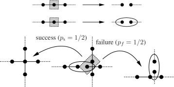
Figure 10: The elementary linear optics tools for building two-dimensional structures from linear cluster chains. From top to bottom: a $\sigma_{z}$ measurement to remove unneeded nodes, a $\sigma_{x}$ measurement to create a redundancy encoded qubit in preparation of type-II fusion. The last figure shows the action of a fusion type-II attempt.

Given the above prescription, depending on $n$, the overall probability $P_{\text{s}}(n)$ of succeeding to prepare an $n\times n$ cluster state can be written as

$$P_{\text{s}}(n)=\pi_{\text{s}}(n)^{n}.$$

Here,

$$\pi_{\text{s}}(n)=p_{\text{s}}^{n}\sum\limits_{k=0}^{(a-1)n}(1-p_{\text{s}})^{k}{n+k-1\choose k}$$

is the success probability to weave a single chain of length $an$ into the carpet of size $n$ with the binomial quantifying the number of ways to distribute $k$ failures on $n$ nodes [34]. $p_{\text{s}}>0$ and $1-p_{\text{s}}$ are the success and failure probabilities for a fusion attempt, respectively. It can be rephrased as the probability to find at least $n$ successful outcomes in $an$ trials,

$$\pi_{\text{s}}(n) = \sum\limits_{k=n}^{an}(1-p_{\text{s}})^{an-k}p_{\text{s}}^{k}{an\choose k}$$

$$= 1-F(n-1,an,p_{\text{s}}).$$

Here, $F$ denotes the standard cumulative distribution function of the binomial distribution [35]. Since $n-1\leq anp_{\text{s}}$ for all $n$, as $a>1/p_{\text{s}}$ is assumed, we can hence bound $\pi_{\text{s}}(n)$ from below by means of Hoeffding’s inequality [36, 37], providing an exponentially decaying upper bound of the tails of the cumulative distribution function. This gives rise to the lower bound

$$\pi_{\text{s}}(n)\geq 1-\exp\left(-\frac{2(anp_{\text{s}}-n+1)^{2}}{an}\right).$$

Now, again since $a>1/p_{\text{s}}$, we have that

$$\pi_{\text{s}}^{n}\geq\left(1-\exp(-cn)\right)^{n}$$

with $c:=2(ap_{\text{s}}-1)/a>0$. Further, for any $k\in\mathbbm{N}$ there exists an $n_{0}\in\mathbbm{N}$ such that for all $n\geq n_{0}$

$$\left(1-\exp(-cn)\right)^{n}>\left(1-1/(kn)\right)^{n}.$$

Noticing

$$\lim_{n\rightarrow\infty}\left(1-1/(kn)\right)^{n}=\mathrm{e}^{-1/k}$$

we can find for any $\varepsilon>0$ a $k$ satisfying $1-\mathrm{e}^{-1/k}<\varepsilon$. Therefore, for any $\varepsilon>0$ it holds that $\lim_{n\rightarrow\infty}P_{\text{s}}>1-\varepsilon$. This ends the argument leading to the appropriate scaling. ∎

Even within the setting of quadratic resources, the appropriate choice for $a$ does have an impact: If the probability of success $p_{\text{s}}$ is too small for a given $a$,

$$1/p_{\text{s}}>a>1,$$

then this will lead to $\lim_{n\rightarrow\infty}P_{\text{s}}(n)=0$, so the preparation of the cluster will eventually fail, asymptotically with certainty. This sudden change of the asymptotic behavior of the resource requirements, leading essentially to either almost unit (almost all cluster states can successfully be prepared) or almost vanishing success probability is a simple threshold phenomenon as in percolation theory. In turn, for a given $a$, $p_{\text{th}}=1/a$ can be taken as a threshold probability: above this threshold almost all preparations will succeed, below it they will fail [38]. This number $a$ essentially dictates the constant factor in front of the quadratic behavior in the scaling of the resource requirements. Needless to say, this depends on $p_{\text{s}}$.

This analysis shows that a two-dimensional cluster state can indeed be prepared using $O(n^{2})$ edges, employing probabilistic quantum gates only. This can be viewed as good news, as it shows that the natural scaling of the use of such resources can indeed be met, with asymptotically negligible error. Previously, only strategies leading to a super-quadratic resource consumption have been known. In turn, any such other scaling of the resources could have been viewed as a threat to the possibility of being able to prepare higher-dimensional cluster states using probabilistic quantum gates.

XI Summary, discussion, and outlook

In this paper, we have addressed the question of how to prepare cluster states using probabilistic gates. The emphasis was put on finding bounds that the optimal strategy necessarily has to satisfy, to identify final bounds on the resource overhead necessary in such a preparation. This issue is particularly relevant in the context of linear optics, where the necessary overhead in resource is one of the major challenges inherent in this type of architecture. It turns out that the way the classical strategy is chosen has a major impact on the resource consumption. By providing these rigorous bounds, we hope to give a guideline to the feasibility of probabilistic state generation. One central observation, e. g., is that for any preparation of linear cluster states using linear optical gates as specified above, one necessarily needs at least five EPR pairs per average gain of one edge. This limit can within these rules no further be undercut. But needless to say, the derived results are also applicable to other architectures, and we tried to separate the general statements from those that focus specifically on linear optical setups.

It is also the hope that the introduced tools and ideas are applicable beyond the exact context discussed in the present paper. There are good reasons to believe that these methods may prove useful even when changing the rules: For example, as fusion type-II can also be used for production of redundancy encoding resource states [6] and linear cluster states in a similar fashion, similar bounds to resource consumption may be derived for these schemes. Due to the fact that fusion type-II does not require photon number resolving detectors, this could be a matter of particular interest for experimental realizations. Also, generalizations of some of the statements for $p_{\text{s}}\neq 1/2$ have been explicitly derived. Other generalizations may well also be proven with the tools developed in this paper.

Concerning lossy operations, we emphasize again that when all EPR pairs are simultaneously created in the beginning, their storage time will be minimized by application of the strategy that optimizes the expected final length. Obviously, the problem of storage using fiber loops or memories is a key issue in any realization. Yet, for a given loss mechanism, it would be interesting to see to what extent a modification of the optimal protocol would follow – compared to the one here assuming perfect operations – depending on the figures of merit chosen. One then expects trade-offs between different desiderata to become relevant [39]. In the way it is done here, decoherence induced by the actual gates employed for the fusion process is also minimized exactly by choosing the optimal strategy of this work: it needs the least number of uses of the underlying quantum gates.

Further, studies in the field of fault tolerance may well benefit from this approach. To start with, one has to be aware that the overhead induced in fully fault-tolerant one-way computing schemes is quite enormous [21]. This is extenuated when considering photon loss only as a source of errors [22, 6]. Yet, methods as the ones presented here will be expected to be useful to very significantly reduce the number of gate invocations in the preparation of the resources.

XII Acknowledgments

We would like to acknowledge discussions with the participants of the LoQuIP conference on linear optical quantum information processing in Baton Rouge in April 2006, organized by J. Dowling. The authors are grateful to A. Feito for a host of comments on a draft version. This work has been supported by the DFG, the EU (QAP), the EPSRC, QIP IRC, Microsoft Research through the European PhD Scholarship Programme, and the EURYI award scheme.

References

- [1] E. Knill, R. Laflamme, and G.J. Milburn, Nature (London) 409, 46 (2001).
- [2] P. Kok, W.J. Munro, K. Nemoto, T.C. Ralph, J.P. Dowling, and G.J. Milburn, Rev. Mod. Phys. 79, 135 (2007); C.R. Myers and R. Laflamme, quant-ph/0512104.
- [3] N. Yoran and B. Reznik, Phys. Rev. Lett. 91, 037903 (2003).
- [4] M.A. Nielsen, Phys. Rev. Lett. 93, 040503 (2004).
- [5] D.E. Browne and T. Rudolph, Phys. Rev. Lett. 95, 010501 (2005).
- [6] T.C. Ralph, A.J.F. Hayes, and A. Gilchrist, Phys. Rev. Lett. 95, 100501 (2005); A. Gilchrist, A.J.F. Hayes, T.C. Ralph, quant-ph/0505125.
- [7] T.B. Pittman, B.C. Jacobs, and J.D. Franson, Phys. Rev. A 64, 062311 (2001).
- [8] J.I. Cirac, A. Ekert, S.F. Huelga, and C. Macchiavello, Phys. Rev. A 59, 4249 (1999).
- [9] J. Eisert, K. Jacobs, P. Papadopoulos, and M.B. Plenio, Phys. Rev. A 62, 052317 (2000); D. Collins, N. Linden, and S. Popescu, ibid. 64, 032302 (2001).
- [10] M.A. Nielsen and I.L. Chuang, Quantum computation and quantum information (Cambridge University Press, Cambridge, 2000); J. Eisert and M.M. Wolf, Quantum computing, in Handbook of nature-inspired and innovative computing (Springer, New York, 2006).
- [11] J. Eisert, Phys. Rev. Lett. 95, 040502 (2005); S. Scheel, W.J. Munro, J. Eisert, K. Nemoto, and P. Kok, Phys. Rev. A 73, 034301 (2006); S. Scheel and K.M.R. Audenaert, New J. Phys. 7, 149 (2005); S. Scheel and N. Lütkenhaus, ibid. 6, 51 (2004); E. Knill, Phys. Rev. A 68, 064303 (2003).
- [12] H.-J. Briegel and R. Raussendorf, Phys. Rev. Lett. 86, 910 (2001); R. Raussendorf and H.-J. Briegel, ibid. 86, 5188 (2001).
- [13] M. Hein, J. Eisert, and H.-J. Briegel, Phys. Rev. A 69, 062311 (2004); M. Van den Nest, J. Dehaene, and B. De Moor, ibid. 69, 022316 (2004); R. Raussendorf, D.E. Browne, and H.-J. Briegel, ibid. 68, 022312 (2003); D. Schlingemann and R.F. Werner, ibid. 65, 012308 (2002).
- [14] M. Hein, W. Dür, J. Eisert, R. Raussendorf, M. Van den Nest, and H.-J. Briegel, quant-ph/0602096; D.E. Browne and H.-J. Briegel, quant-ph/0603226.
- [15] P. Walther, K.J. Resch, T. Rudolph, E. Schenck, H. Weinfurter, V. Vedral, M. Aspelmeyer, and A. Zeilinger, Nature 434, 169 (2005); N. Kiesel, C. Schmid, U. Weber, G. Toth, O. Gühne, R. Ursin, and H. Weinfurter, Phys. Rev. Lett. 95, 210502 (2005).
- [16] The term “EPR pair” is to be understood in the sense of dual rail encoding introduced in Section III.2.
- [17] S.D. Barrett and P. Kok, Phys. Rev. A 71, 060310(R) (2005); Y.L. Lim, S.D. Barrett, A. Beige, P. Kok, and L.C. Kwek, Phys. Rev. A 73, 012304 (2006).
- [18] S.C. Benjamin, Phys. Rev. A 72, 056302 (2005); Q. Chen, J. Cheng, K.-L. Wang, and J. Du, ibid. 73, 012303 (2006); G. Gilbert, M. Hamrick, and Y.S. Weinstein, ibid. 73, 064303 (2006).
- [19] L.M. Duan and R. Raussendorf, Phys. Rev. Lett. 95, 080503 (2005).
- [20] K. Kieling, D. Gross, and J. Eisert, J. Opt. Soc. Am. B 24, 184 (2007).
- [21] C.M. Dawson, H.L. Haselgrove, and M.A. Nielsen, Phys. Rev. Lett. 96, 020501 (2006); C.M. Dawson, H.L. Haselgrove, and M.A. Nielsen, Phys. Rev. A 73, 052306 (2006); P. Aliferis and D.W. Leung, Phys. Rev. A 73, 032308 (2006); R. Raussendorf, J. Harrington, and K. Goyal, quant-ph/0510135.
- [22] M. Varnava, D.E. Browne, and T. Rudolph, Phys. Rev. Lett. 97, 120501 (2006).
- [23] S.C. Benjamin, J. Eisert, and T.M. Stace, New J. Phys. 7, 194 (2005).
- [24] S. Bose, P.L. Knight, M.B. Plenio, and V. Vedral, Phys. Rev. Lett. 83, 5158 (1999); D.E. Browne, M.B. Plenio, and S.F. Huelga, ibid. 91, 067901 (2003).
- [25] N.G. Van Kampen, Stochastic processes in physics and chemistry (North Holland, Amsterdam, 1992).
- [26] S. Boyd and L. Vandenberghe, Convex optimization (Cambridge University Press, Cambridge, 2004).
- [27] Compare also “An EPR pair is nothing but a cluster state of length one”, C.M. Dawson, LoQUIP, Baton Rouge, April 2006.
- [28] J. Calsamiglia and N. Lütkenhaus, Appl. Phys. B 72, 67–71 (2001).
- [29] N.J.A. Sloane, http://www.research.att.com/projects/OEIS? Anum=A000070.
- [30] K. Kieling, Linear optical methods in quantum information processing (Diploma thesis, University of Potsdam, 2005).
-
[31]
With one obtains
-
[32]