On Decoherence in Quantum Clock Synchronization

Abstract

We study two quantum versions of the Eddington clock-synchronization protocol in the presence of decoherence. The first protocol uses maximally entangled states to achieve the Heisenberg limit for clock synchronization. The second protocol achieves the limit without using entanglement. We show the equivalence of the two protocols under any single-qubit decoherence model that does not itself provide synchronization information.

I Introduction

The problem of synchronizing distant clocks is of fundamental interest in physics, as well as having important applications in metrology and engineering. Suppose Alice and Bob are two space-like-separated observers who wish to synchronize their clocks. We consider the situation in which the two observers share an inertial reference frame and have two classical clocks ticking at the same rate. Classically, there are two canonical protocols for synchronizing clocks, one due to Einstein, which is based on sending light signals, and one due to Eddington, which involves exchanging clocks. The accuracy with which Alice and Bob can synchronize their clocks classically, using either procedure, scales as $1/\sqrt{n}$, where $n$ is the number of times the protocol is executed. This scaling is generally known as the Standard Quantum Limit (SQL) Braginsky and Vorontsov (1975); Caves et al. (1980); Giovannetti et al. (2004).

Over the last decade, there has been considerable interest in studying quantum versions of these protocols Bollinger et al. (1996); Huelga et al. (1997); Jozsa et al. (2000); Chuang (2000); Preskill (2000); Yurtsever and Dowling (2002); Revzen and Mann (2003); Giovannetti et al. (2004); de Burgh and Bartlett (2005). Some of this work was motivated solely by the quest for better frequency standards, whereas others aimed at beating the SQL. It has now been shown that quantum clock-synchronization protocols can perform better than classical ones and that the scaling can be improved in the quantum case to $1/n$, the so-called Heisenberg Limit.

There are two interesting quantum versions of the Eddington protocol for clock synchronization, which classically involves Alice (adiabatically) sending to Bob a “watch” synchronized with her clock. In quantum versions of this protocol, the watch is a time evolving observable of one or more qubits. In one version, these “ticking qubits” are prepared in a maximally entangled “cat” state Bollinger et al. (1996); Jozsa et al. (2000); entanglement is the resource that allows this protocol to achieve the Heisenberg Limit. An alternative quantum version of the Eddington protocol achieves the Heisenberg Limit by using multiple, coherent exchanges of a single ticking qubit between Alice and Bob de Burgh and Bartlett (2005); in this protocol quantum coherence is identified as the resource that provides an advantage over the classical protocol.

Our aim in this paper is to compare and contrast the performance of the two protocols in the presence of decoherence in the quantum channel between Alice and Bob. It is known that both quantum versions of the Eddington protocol use the same amount of total qubit communication de Burgh and Bartlett (2005). Our study investigates the status of this similarity in the case of a non ideal quantum channel between Alice and Bob, which is expected to degrade the performance of the protocols. We find that the two protocols are affected in the same way by any single-qubit decoherence process that does not itself provide useful synchronization information.

The paper is structured as follows. In Sec. II we review the two quantum clock-synchronization protocols and touch on the question of whether anything more than a shared inertial reference frame is required for Alice and Bob to synchronize their clocks. Section III describes our decoherence model. Our results are presented in Sec. IV, and we conclude in Sec. V.

II Two Quantum Clock-Synchronization Protocols

II.1 Assumptions and conventions

Prior to describing clock-synchronization protocols, we need to describe our assumptions and fix some conventions. The problem is to synchronize two classical clocks, one maintained by Alice, which reads time $t_{A}$, and one by Bob, which reads time $t_{B}$. We assume that Alice’s and Bob’s clocks tick at the same rate, so the problem is wholly that of determining the constant offset $t_{BA}=t_{B}-t_{A}$.

Since we are considering quantum versions of the Eddington protocol, Alice and Bob synchronize their clocks by exchanging ticking qubits. We think of a ticking qubit as being two atomic levels, whose free Hamiltonian is

$$H_{0}={\frac{\hbar\omega}{2}}Z={\frac{\hbar\omega}{2}}\bigl{(}|0\rangle\langle 0|-|1\rangle\langle 1|\bigr{)}\;,$$ (1)

where $Z$ is the Pauli $\sigma_{z}$ operator and $|0\rangle$ and $|1\rangle$ are the upper and lower energy eigenstates. Agreeing on the atomic free Hamiltonian means, first, that Alice and Bob agree on the $Z$ axis of the Bloch sphere that describes the two-dimensional atomic Hilbert space and, second, that they share the transition frequency $\omega$. This frequency is an expression of the fixed frequency unit that the parties share as a consequence of having clocks that tick at the same rate.

To exchange information through the ticking qubits, Alice and Bob must perform operations on the qubits, such as setting them ticking, stopping their ticking, and changing the phase of their ticking. All these operations can be performed by illuminating a qubit with a laser tuned to the transition frequency. The Hamiltonian for this interaction, in the interaction picture, is the Rabi Hamiltonian

$$H_{\rm Rabi}=\frac{\hbar\Omega}{2}\bigl{(}e^{-i\varphi_{P}}|0\rangle{\langle 1|}+e^{i\varphi_{P}}|1\rangle{\langle 0|}\bigr{)}=\frac{\hbar\Omega}{2}\bigl{(}X\cos\varphi_{P}+Y\sin\varphi_{P})\;.$$ (2)

Here $X$ and $Y$ denote the Pauli $\sigma_{x}$ and $\sigma_{y}$ operators, $\Omega$ is the Rabi frequency, and $\varphi_{P}$ is the phase of the driving laser relative to the zero of clock $P$. In Bloch-sphere language, the Rabi Hamiltonian generates a rotation at frequency $\Omega$ about an axis in the equatorial plane that makes an angle $\varphi_{P}$ with the $X$ axis.

Since Alice and Bob do not share clocks with a common zero, they have different phase references $\varphi_{A}$ and $\varphi_{B}$ and, hence, different Bloch-sphere $X$ and $Y$ axes. The problem of clock synchronization reduces to estimating the phase offset $\varphi_{BA}=\varphi_{B}-\varphi_{A}=\omega t_{BA}\equiv\varphi$. When $\varphi\neq 0$, Alice and Bob describe states and operations differently. Their separate descriptions are related by a rotation through angle $\varphi$ about the common $Z$ axis de Burgh and Bartlett (2005). An operator $O_{A}$ in Alice’s description is considered by Bob to be the operator

$$O_{B}=e^{-iZ\varphi/2}O_{A}e^{iZ\varphi/2}\;.$$ (3)

It might seem that the sharing of a common Bloch-sphere $Z$ axis requires a preferred spatial direction shared by the two parties. It is, however, possible to imagine a situation in which both $|0\rangle$ and $|1\rangle$ are zero-angular-momentum levels of an atom, in which case the Hamiltonian (2) has no preferred spatial direction. Unfortunately, electric-dipole ($E1$) selection rules forbid any $J^{\prime}=0\rightarrow J=0$ transition. To circumvent this, one could use a coherent two-photon Raman process via an intermediate state to drive the forbidden transition. Although this process does involve fixed orientations in space, since the Raman transitions are carried out by Alice and Bob independently and locally in their respective laboratories, they need not share a common spatial axis. We thus do not need the alignment of any spatial axes for time synchronization. This is in harmony with the process of aligning spatial reference frames, which does not require any time synchronization Rudolph and Grover (2003).

II.2 Cat-state entangled protocol

Of the schemes designed to beat the SQL, one of the earliest uses the entangled “cat” state of $n$ qubits Bollinger et al. (1996). Starting with the state $|000\ldots 0\rangle$, Alice prepares the cat state Huelga et al. (1997),

$$|\psi_{A}\rangle=\frac{1}{\sqrt{2}}\bigl{(}|000\ldots 0\rangle+|111\ldots 1\rangle\bigr{)}_{A}\;,$$ (4)

by performing a $90^{\circ}$ rotation about the $Y_{A}$ axis (or a Hadamard gate $H_{A}$) on the first qubit, followed by controlled spin flips ($X_{A}$), controlled by the first qubit and targeted on each of the other qubits. Alice sends the $n$ qubits to Bob, who measures the observable $O_{B}=X_{B}^{\otimes n}$ (alternatively, Bob can reverse the steps that prepared the cat state, but using his operations, of course, and then measure $Z$ on the first qubit). Since $O_{B}$ is a binary observable, its distribution is determined by its expectation value,

$${\langle\psi_{A}|}O_{B}|\psi_{A}\rangle=\cos(n\phi_{BA})\;,$$ (5)

which corresponds to Ramsey-fringe probabilities

$$p_{\pm}=[1\pm\cos(n\phi_{BA})]/2$$ (6)

for results $\pm 1$. This leads to a nominal uncertainty in determining $\varphi$ given by

$$\Delta\varphi=\frac{\Delta O_{B}}{|d\langle O_{B}\rangle/d\varphi|}=\frac{1}{n}\;,$$ (7)

where $\Delta O_{B}=\sin(n\varphi)$ is the uncertainty in $O_{B}$.

Since the probabilities (6) are periodic in $\varphi_{BA}$ with fringe period $2\pi/n$, determining $\varphi$ within the uncertainty (7) requires one already to know $\varphi$ to an accuracy $2\pi/n$. One gets around this problem by using an extended protocol, which ultimately leads to a Heisenberg-limited sensitivity. Defining $\omega t_{BA}=\varphi=\pi T$ and writing the dimensionless time offset $T$ in binary form as $T=0.t_{1}t_{2}\ldots\,$, the problem of synchronizing clocks becomes that of determining the sequence of bits in the binary decomposition. (We are assuming that Alice and Bob already know $\varphi$ to within $\pi$, but notice that Bob could determine the bit $t_{0}$ in $T=t_{0}.t_{1}t_{2}\ldots$ by running the bare protocol several times with a single unentangled qubit). If the sequence is known through the $(j-1)$th bit, ascertaining the $j$th bit can be accomplished by using the cat state with $2^{j}$ qubits. Of course, Alice and Bob must repeat the bare protocol several times to build up the statistics to determine the $j$th bit. The statistical uncertainty in $\varphi$, given by $1/(2^{j}\sqrt{\nu})$, where $\nu$ is the number of repetitions, should be small compared to $\pi/2^{j}$; i.e., $\pi\sqrt{\nu}$ should be somewhat larger than 1 in order to determine the $j$th bit reliably.

Our conclusion is that to determine the first $k\gg 1$ bits of $T$ requires running the bare protocol $\nu$ times for each bit, using $2^{j}$ entangled qubits to determine the $j$th bit, for a total of $N=2\nu(2^{k}-1)$ qubits. The resulting accuracy in determining $t_{BA}$,

$$\delta t_{BA}=\frac{1}{\omega}\frac{\pi}{2^{k}}\simeq\frac{2\pi\nu}{\omega N}\;,$$ (8)

has the scaling of the Heisenberg limit.

II.3 Coherent-transport protocol

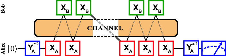
Figure 1: (Color online) The coherent-transport protocol in pictures. The $90^{\circ}$ rotation about $Y_{A}$, denoted here by $Y_{A}^{\pi/2}$, takes state $|0\rangle$ to $(|0\rangle+|1\rangle)_{A}/\sqrt{2}$; $X_{A}$ and $X_{B}$ are $180^{\circ}$ rotations by Alice Bob about their respective $X$ axes. A final $90^{\circ}$ rotation by Alice is followed by a measurement of $Z$. An alternative end point for the protocol is for Alice to return the qubit one last time to Bob, who does a $90^{\circ}$ rotation about his axis $Y_{B}$, followed by a measurement of $Z$.

The procedure outlined in the preceding subsection uses entanglement of a larger and larger number of qubits to read out successive digits of $T$, so we call it the entanglement protocol. The use of entanglement is in line with the notion that entanglement is necessary to beat the SQL. There exist protocols, however, that do not require entanglement to beat the SQL, relying instead on coherent exchanges of a single qubit. The first such protocol was presented by Rudolph and Grover Rudolph and Grover (2003) for the task of aligning spatial reference axes. The underlying idea of multiple exchanges was considered much earlier, in a wider context, by Salecker and Wigner Salecker and Wigner (1958). Rudolph and Grover’s protocol was adapted to the problem of synchronizing clocks by de Burgh and Bartlett de Burgh and Bartlett (2005).

In this protocol Alice prepares a qubit in the state $|0\rangle$ and applies her $90^{\circ}$ rotation about $Y_{A}$ (or her Hadamard gate $H_{A}$) to put the qubit in the state

$$|\phi_{A}\rangle=(|0\rangle+|1\rangle)_{A}/\sqrt{2}\;.$$ (9)

Alice then sends the qubit to Bob, who performs his operation $X_{B}$. Bob sends the qubit back to Alice, and she performs her operation $X_{A}$. The result of this exchange is that they jointly execute the operation

$$X_{A}X_{B}=X_{A}(e^{-iZ\varphi/2}X_{A}e^{iZ\varphi/2})=e^{iZ\varphi}\;.$$ (10)

Alice and Bob continue ping-ponging the qubit in this way. If, after $r$ such exchanges, Alice measures the observable $O_{A}=X_{A}$ (alternatively, she could undo the initial rotation about $Y_{A}$ and then measure $Z$), the expectation value of $O_{A}$ is $\langle\phi_{A}|e^{-iZr\varphi}X_{A}e^{iZr\varphi}|\phi_{A}\rangle=\cos(2\,r\varphi)$. If, instead, Alice returns the qubit to Bob, who measures $O_{B}=X_{B}$ (alternatively, Bob could undo the initial $Y$ rotation, using his axis $Y_{B}$, of course, and then measure $Z$), the expectation value of the measured observable is $\langle\phi_{A}|e^{-iZr\varphi}X_{B}e^{iZr\varphi}|\phi_{A}\rangle=\cos[(2\,r+1)\varphi]$.

We call this the coherent-transport protocol because the qubit is shuttled coherently back and forth between Alice and Bob. The number of uses of the qubit channel, $n=2r$ or $n=2r+1$, plays exactly the same role in this protocol as does the number of qubits in the entangled protocol. Indeed, since each qubit in the entangled protocol traverses the qubit channel once, $n$ denotes the number of uses of the qubit channel for both protocols.

The coherent-transport protocol can be generalized to an extended protocol which reads out successive bits of the dimensionless time offset $T$, in precise analogy to the extended entangled protocol. In the extended protocol, to determine the $j$th bit of $T$, Alice and Bob exchange the qubit $r=n/2=2^{j-1}$ times, running the bare protocol several times to build up sufficient statistics. The coherent-transport protocol achieves exactly the same sensitivity (8) as the entangled protocol, with $n$ being the total number of uses of the quantum channel. Notice that in the extended protocol, Alice makes all the measurements and ends up with the measured value of $T$.

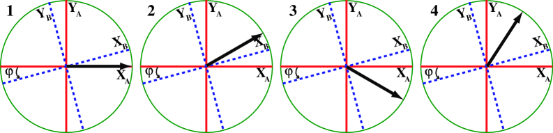
Figure 2: (Color online) How the coherent-transport protocol works. In 1, the Bloch vector (black arrow) of the qubit is shown after Alice has done the initial rotation $Y^{\pi/2}_{A}$, which leaves the qubit polarized along Alice’s axis $X_{A}$. Bob’s axes $X_{B}$ and $Y_{B}$ (dashed blue lines) are oriented at an angle $\varphi$ relative to Alice’s axes (solid red lines). The qubit is sent to Bob who does a $180^{\circ}$ rotation about $X_{B}$. After this rotation, the Bloch vector, depicted in 2, has rotated by an angle $2\varphi$ relative to $X_{A}$. The Bloch vector after Alice has done her $X_{A}$ operation is shown in 3, while in 4, the Bloch vector after a further $X_{B}$ operation is shown. We see that each time Alice and Bob send the qubit back and forth once, the Bloch vector is rotated by angle $-2\varphi$. The original angle between the two sets of axes is amplified and recorded in the state of the qubit when it is exchanged several times between Alice and Bob.

The entangled protocol relies on entanglement to beat the SQL, whereas the coherent-transport protocol relies on maintaining the coherence as it is shuttled back and forth between Alice and Bob. The former requires maintaining spatial coherence among many qubits, whereas the latter requires maintaining the temporal coherence of a single qubit. Both schemes are vulnerable to decoherence in the quantum channel between Alice and Bob. For the entangled protocol, calculations done using a specific decoherence model revealed the deleterious effects of decoherence and showed that other initial entangled states perform better than the cat state Huelga et al. (1997). The effect of decoherence on estimating the time difference is, not surprisingly, related to the question of the statistical distinguishability of neighboring states Braunstein and Caves (1994). The performance of the coherence-transport protocol also deteriorates in the presence of decoherence in the channel. Both protocols are able to beat the SQL in the presence of a decoherence in the channel, albeit only up to a limited precision governed by the level of noise in the channel.

Up till now, there has been no systematic study of the two quantum clock-synchronization protocols in the presence of a general decoherence model. We provide such an analysis in the next section, where we consider the most general single-qubit decoherence process possible for the scenario at hand and study its effect on the two protocols. The study makes evident that the two protocols are essentially equivalent in their sensitivity to decoherence. The one difference that emerges prompts us to propose a variation of the entangled protocol, which makes it precisely equivalent to the coherent-transport protocol in the presence of decoherence.

III Decoherence Model

We model decoherence in the quantum channel as a completely positive, trace-preserving (CPTP) linear map or superoperator (Nielsen and Chuang, 2000, Chapter 8), which acts on a qubit each time it traverses the quantum channel. This means that we ignore possible spatially or temporally correlated decoherence that may occur in the two clock-synchronization protocols. A CPTP map $\mathcal{E}$ acting on a single qubit is defined in terms of its action on the operator basis set $\{\sigma_{\xi}\}=\{I,Z,X,Y\}$, i.e.,

$$\mathcal{E}(\sigma_{\xi})=\sum_{\eta}\sigma_{\eta}\mathcal{E}_{\eta\xi}\;.$$ (11)

In writing this representation, we assume that $X$ and $Y$ are as defined by Alice. The $4\times 4$ matrix that represents $\mathcal{E}$ has the general form (Nielsen and Chuang, 2000, Chapter 8)

$$||\mathcal{E}_{\eta\xi}||=\left(\begin{array}[]{cccc}1&0&0&0\\ t_{Z}&\phantom{R_{2}SR_{1}}&\phantom{R_{2}SR_{1}}&\phantom{R_{2}SR_{1}}\\ t_{X}&&R_{2}SR_{1}&\\ t_{Y}&&&\end{array}\right)\;,$$ (12)

where $R_{1}$ and $R_{2}$ are three-dimensional Bloch rotation matrices and $S$ is a three-dimensional diagonal matrix,

$$S=\left(\begin{array}[]{ccc}s_{Z}&0&0\\ 0&s_{X}&0\\ 0&0&s_{Y}\end{array}\right)\;,$$ (13)

whose diagonal elements satisfy $|s_{j}|\leq 1$.

We can define a related operation $\mathcal{F}$ whose matrix representation is

$$||\mathcal{F}_{\eta\xi}||=\left(\begin{array}[]{cccc}1&0&0&0\\ t_{Z}&s_{Z}&0&0\\ t_{X}&0&s_{X}&0\\ t_{Y}&0&0&s_{Y}\end{array}\right)\;.$$ (14)

The action of $\mathcal{E}$ is that of $\mathcal{F}$ preceded by rotation $R_{1}$ and succeeded by rotation $R_{2}$, i.e.,

$$\mathcal{E}(\rho)=U_{2}\mathcal{F}\bigl{(}U_{1}\rho U_{1}^{\dagger}\bigr{)}U_{2}^{\dagger}\;,$$ (15)

where $U_{1}$ and $U_{2}$ are the unitary operators corresponding to the Bloch rotations $R_{1}$ and $R_{2}$.

In the interaction picture, clock synchronization reduces to finding the angle $\varphi$ between Alice’s axis $X_{A}$ and Bob’s axis $X_{B}$. We assume that the channel itself, through the decoherence it produces, should not provide any information about $\varphi$. Formally, this means that the map $\mathcal{E}$ should commute with rotations about the common $Z$ axis. This implies, first, that $t_{X}=t_{Y}=0$ (we let $t_{Z}=t$) and, second, that the pre- and post-rotations $R_{1}$ and $R_{2}$ must be rotations about the $Z$ axis and $s_{X}=s_{Y}=\lambda$ (we let $s_{Z}=s$). With these restrictions, $R_{1}$ and $R_{2}$ commute with $S$, so we can combine them into a single (pre- or post-) rotation $R=R_{2}R_{1}$ about the $Z$ axis, which we take to be a rotation by angle $\alpha$. The matrix (11) of our CPTP map now takes the form

$$||\mathcal{E}_{\eta\xi}||=\left(\begin{array}[]{cccc}1&0&0&0\\ t&s&0&0\\ 0&0&\lambda\cos\alpha&-\lambda\sin\alpha\\ 0&0&\lambda\sin\alpha&\lambda\cos\alpha\end{array}\right)\;.$$ (16)

The matrix of the related operation $\mathcal{F}$ is even simpler,

$$||\mathcal{F}_{\eta\xi}||=\left(\begin{array}[]{cccc}1&0&0&0\\ t&s&0&0\\ 0&0&\lambda&0\\ 0&0&0&\lambda\end{array}\right)\;,$$ (17)

and corresponds to a displacement of the Bloch sphere by a distance $t$ in the $Z$ direction, compression of the Bloch sphere by a factor $s$ along the $Z$ axis, and compression by a factor $\lambda$ in the equatorial plane. The operation of $\mathcal{E}$ is that of $\mathcal{F}$ with a preceding or succeeding rotation by $\alpha$ about the $Z$ axis, i.e.,

$$\mathcal{E}(\rho)=e^{-iZ\alpha/2}\mathcal{F}(\rho)e^{iZ\alpha/2}=\mathcal{F}\bigl{(}e^{-iZ\alpha/2}\rho e^{iZ\alpha/2}\bigr{)}\;.$$ (18)

The channel decoherence acts separately in the operator subspace spanned by $I$ and $Z$ and the subspace spanned by $X$ and $Y$. In the two clock-synchronization protocols described in Sec. II, the last step is a measurement by Alice or Bob of an operator in the equatorial plane of the Bloch sphere. As a result, we are only interested in the part of the output density operator that lies in the $X$-$Y$ subspace. Because $\mathcal{E}$ acts separately in the $I$-$Z$ and $X$-$Y$ subspaces, this means we only need to consider the part of $\mathcal{E}$ that acts in the $X$-$Y$ subspace.

Formally, we deal with this by introducing a superoperator projector $\Pi$ that projects any operator into the operator subspace spanned by $X$ and $Y$:

$$\Pi(O)=\Pi(a_{0}I+a_{Z}Z+a_{X}X+a_{Y}Y)=a_{X}X+a_{Y}Y\;.$$ (19)

Notice that it does not matter whether we use Alice’s or Bob’s $X$ and $Y$ operators to define $\Pi$. The action of $\Pi$ can be written in two other useful forms:

$$\Pi(O)=\frac{1}{2}(O-ZOZ)=|0\rangle\langle 1|\langle 0|O|1\rangle+|1\rangle\langle 0|\langle 1|O|0\rangle\;.$$ (20)

The effect of $\Pi$ is to remove the diagonal matrix elements of $O$ in the $Z$ basis, leaving the off-diagonal matrix elements. The map is neither trace preserving nor completely positive.

For our purposes, the crucial property of $\Pi$ is that it is Hermitian relative to the operator inner product, i.e.,

$${\rm{Tr}}\bigl{(}N^{\dagger}\Pi(O)\bigr{)}={\rm{Tr}}\Bigl{(}\bigl{(}\Pi(N)\bigr{)}^{\dagger}O\Bigr{)}\;.$$ (21)

It is also easy to see that $\Pi\circ\mathcal{F}(O)=\lambda\,\Pi(O)$, from which it follows that

$$\Pi\circ\mathcal{E}(O)=\lambda\,e^{-iZ\alpha/2}\Pi(O)e^{iZ\alpha/2}\;.$$ (22)

Only the rotation $\alpha$ and the compression $\lambda$ in the equatorial plane have any effect on our protocols, and they contribute in a very straightforward way to the relevant action of $\mathcal{E}$. The displacement $t$ and the compression $s$ do not appear in the relevant action of $\mathcal{E}$, although they can have an indirect effect through the requirement of complete positivity, which means that their values constrain the possible value of $\lambda$.

The compression $\lambda$ can come, for example, from random spin flips or phase changes during transit through the channel. The rotation by $\alpha$ is not really a decoherence effect at all; it is an unknown, but systematic phase shift produced by the quantum channel, which can mimic the phase offset the Alice and Bob are trying to determine. It might arise, for example, from a shift of the energy difference between the two levels as a qubit traverses the channel. In a real situation, both $\lambda$ and $\alpha$ might vary from one use of the channel to the next, but we assume they are constant for the analysis in the next section.

IV Effect of decoherence

This section contains the main results of the paper. We analyze the entangled protocol and the coherent-transport protocol in turn.

IV.1 Entangled protocol

The density matrix for the $n$-qubit cat state can be written as Shaji and Caves (2006)

$$\rho_{\rm cat}=\frac{1}{2^{n+1}}\left(\bigotimes_{j=1}^{n}(I_{j}+Z_{j})+\bigotimes_{j=1}^{n}(I_{j}-Z_{j})+\bigotimes_{j=1}^{n}(X_{j}+iY_{j})+\bigotimes_{j=1}^{n}(X_{j}-iY_{j})\right)\;.$$ (23)

The effect of the channel is studied by analyzing its effect on the four terms. Recall that the final measurement by Bob is $O_{B}=X_{B}^{\otimes n}$; since this picks up only the off-diagonal elements in $\mathcal{E}^{\otimes n}(\rho_{\rm cat})$, we can study the effect of the map by considering only the last two terms in Eq. (23).

Formally, we can write

$$\langle O_{B}\rangle={\rm{Tr}}\bigl{(}X_{B}^{\otimes n}\mathcal{E}^{\otimes n}(\rho_{\rm cat})\bigr{)}={\rm{Tr}}\bigl{(}\Pi^{\otimes n}(X_{B}^{\otimes n})\,\mathcal{E}^{\otimes n}(\rho_{\rm cat})\bigr{)}={\rm{Tr}}\bigl{(}X_{B}^{\otimes n}\Pi^{\otimes n}\circ\mathcal{E}^{\otimes n}(\rho_{\rm cat})\bigr{)}\;.$$ (24)

The final form shows that we can discard the first two terms in Eq. (23). The contribution of the third term to the expectation value is

$$\frac{1}{2^{n+1}}{\rm{Tr}}\!\left(\bigotimes_{j=1}^{n}X_{B,j}\Pi\circ\mathcal{E}(X_{A,j}+iY_{A,j})\right)=\frac{1}{2^{n+1}}\Bigl{(}{\rm{Tr}}\bigl{(}X_{B}\Pi\circ\mathcal{E}(X_{A}+iY_{A})\bigr{)}\Bigr{)}^{n}\;.$$ (25)

The use of Alice’s operators $X_{A}$ and $Y_{A}$ here is a consequence of the fact that Alice prepares the initial cat state.

We can now proceed to calculate the term in large parentheses in Eq. (25):

$${\rm{Tr}}\bigl{(}X_{B}\Pi\circ\mathcal{E}(X_{A}+iY_{A})\bigr{)} = \lambda\,{\rm{Tr}}\bigl{(}X_{B}e^{-iZ\alpha/2}(X_{A}+iY_{A})e^{iZ\alpha/2}\bigr{)}$$ (26)

$$= \lambda\,{\rm{Tr}}\bigl{(}e^{-iZ\varphi/2}X_{A}e^{iZ\varphi/2}e^{-iZ\alpha/2}(X_{A}+iY_{A})e^{iZ\alpha/2}\bigr{)}$$

$$= \lambda\,{\rm{Tr}}\bigl{(}e^{-iZ(\varphi-\alpha)}(I-Z)\bigr{)}$$

$$= 2\lambda\langle 1|e^{-iZ(\varphi-\alpha)}|1\rangle$$

$$= 2\lambda\,e^{i(\varphi-\alpha)}\;.$$

Thus the contribution of third term in Eq. (25) to $\langle O_{B}\rangle$ is $\lambda^{n}e^{in(\varphi-\alpha)}/2$, and the fourth term contributes the complex conjugate.

All this yields an expectation value

$$\langle O_{B}\rangle=\langle X_{B}^{\otimes n}\rangle=\lambda^{n}\cos[n(\varphi-\alpha)]\;.$$ (27)

The effect of the equatorial plane decoherence is to reduce the fringe visibility by an exponential factor $\lambda^{n}$; this exponential dependence expresses the extreme sensitivity of the entangled protocol to decoherence in the equatorial plane. An unknown, systematic phase shift $\alpha$ is indistinguishable from the phase offset Alice and Bob are trying to determine and thus limits Bob’s ability to determine $\varphi$, even in the absence of equatorial plane decoherence, i.e., $\lambda=1$. We set aside this problem for the present, assuming $\alpha=0$, but return to it after our analysis of decoherence in the coherent-transport protocol.

The uncertainty in $O_{B}$,

$$\Delta O_{B}=\sqrt{1-\lambda^{2n}\cos^{2}(n\varphi)}\;,$$ (28)

yields a nominal uncertainty in the estimate of $\varphi$,

$$\Delta\varphi=\frac{\Delta O_{B}}{|d\langle O_{B}\rangle/d\varphi|}=\frac{\sqrt{1-\lambda^{2n}\cos^{2}(n\varphi)}}{n\lambda^{n}\sin(n\varphi)}\;.$$ (29)

The uncertainty (29), unlike the $\lambda=1$ limit of Eq. (7), depends on $\varphi$ and, indeed, blows up when $n(\varphi-\alpha)$ is a multiple of $\pi$, i.e., when one happens to be at maximum or minimum of the fringe pattern. This is a purely technical problem, which can be overcome in a variety of ways. For example, in the extended protocol outlined in Sec. II.2, in which Bob runs the bare protocol several times to determine each bit of $T=\varphi/2\pi$, he can alternate measurements of $X_{B}^{\otimes n}$ with measurements of $Y_{B}^{\otimes n}$, for which $\langle Y_{B}^{\otimes n}\rangle=-\lambda^{n}\sin[n(\varphi-\alpha)]$. Sampling from fringe patterns $90^{\circ}$ out of phase in this way allows Bob always to determine $\varphi$ with an uncertainty close to optimal, i.e., $\Delta\varphi\simeq 1/n\lambda^{n}$. Comparing this bare sensitivity with the sensitivity achieved by using $n$ unentangled qubits, $1/\sqrt{n}\lambda$, one sees $\lambda$ must be very close to 1 in order to receive any benefit from entangling substantial numbers of qubits.

IV.2 Coherent-transport protocol

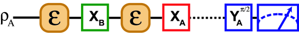
Figure 3: (Color online) A single ping-pong of the qubit between Alice and Bob in the coherent-transport protocol, with the decohering CPTP map included in the two traverses of the quantum channel.

A single exchange of the qubit between Alice and Bob in the coherent-transport protocol is shown in Fig. 3, where

$$\rho_{A}=|\phi_{A}\rangle\langle\phi_{A}|={\frac{1}{2}}(I+X_{A})$$ (30)

is the initial state (9) prepared by Alice. The qubit’s state on its return to Alice is

$$X_{A}\mathcal{E}\bigl{(}X_{B}\mathcal{E}(\rho_{A})X_{B}\bigr{)}X_{A}=\mathcal{G}(\rho_{A})\;.$$ (31)

Here we introduce the overall CPTP map $\mathcal{G}$ for a single exchange. What we want to calculate is the expectation value of the observable $X_{A}$ measured by Alice after this single exchange. Using $\Pi(X_{A})=X_{A}$ and Eq. (21), we can write this expectation value as

$$\langle X_{A}\rangle={\rm{Tr}}\bigl{(}X_{A}\mathcal{G}(\rho_{A})\bigr{)}={\rm{Tr}}\bigl{(}X_{A}\Pi\circ\mathcal{G}(\rho_{A})\bigr{)}\;.$$ (32)

Now we use Eq. (22) and the fact that $\Pi$ commutes with application of $X_{A}$ and $X_{B}$ to write

$$\Pi\circ\mathcal{G}(\rho_{A})=\lambda^{2}X_{A}e^{-iZ\alpha/2}X_{B}e^{-iZ\alpha/2}\Pi(\rho_{A})e^{iZ\alpha/2}X_{B}e^{iZ\alpha/2}X_{A}\;.$$ (33)

Equation (10) now gives

$$X_{A}e^{-iZ\alpha/2}X_{B}e^{-iZ\alpha/2}=X_{A}X_{B}=e^{iZ\varphi}\;,$$ (34)

from which we have

$$\Pi\circ\mathcal{G}(\rho_{A})=\lambda^{2}e^{iZ\varphi}\Pi(\rho_{A})e^{-iZ\varphi}={\frac{1}{2}}\lambda^{2}e^{iZ\varphi}X_{A}e^{-iZ\varphi}={\frac{1}{2}}\lambda^{2}X_{A}e^{-iZ2\varphi}\;.$$ (35)

Thus the desired expectation value is

$$\langle X_{A}\rangle={\frac{1}{2}}\lambda^{2}{\rm{Tr}}(e^{-iZ2\varphi})=\lambda^{2}\cos(2\varphi)\;.$$ (36)

These considerations are easily generalized to $r$ exchanges. The qubit state after $r$ exchanges is $\mathcal{G}^{r}(\rho_{A})$. Equation (35) generalizes to

$$\Pi\circ\mathcal{G}^{r}(\rho_{A})=\lambda^{2\,r}e^{iZr\varphi}\Pi(\rho_{A})e^{-iZr\varphi}={\frac{1}{2}}\lambda^{2\,r}X_{A}e^{-iZ2\,r\varphi}\;,$$ (37)

which means that the expectation value of a measurement of $X_{A}$ by Alice after $r$ exchanges is

$$\langle X_{A}\rangle={\rm{Tr}}\bigl{(}X_{A}\Pi\circ\mathcal{G}^{r}(\rho_{A})\bigr{)}=\lambda^{2\,r}\cos(2\,r\varphi)\;.$$ (38)

Comparison with the comparable expectation value (27) for the entangled protocol shows that the coherent-transport protocol has the same behavior as the entangled protocol, with $n=2r$, except that the coherent- transport protocol is insensitive to the systematic channel phase shift $\alpha$. In accordance with our discussion of the entangled protocol, this means that the coherent-transport protocol can determine the phase offset with uncertainty $\Delta\varphi\simeq 1/n\lambda^{n}$.

The insensitivity of the coherent-transport protocol to $\alpha$ is noteworthy and deserves discussion. The insensitivity to $\alpha$ comes about because Bob’s spin flip $X_{B}$ has the effect that the phase shift accumulated by the qubit as it traverses the channel from Alice to Bob is canceled by phase shift on the return leg to Alice. A slight modification of the entangled protocol allows it to take advantage of the same effect. Alice prepares $n/2$ qubits in the cat state. She sends the qubits to Bob, who performs his spin flip $X_{B}$ on each qubit and sends them all back to Alice. Alice then measures $X_{A}^{\otimes n/2}$. This combination of the entangled and coherent-transport protocols achieves the same Heisenberg-limited sensitivity as the coherent-transport protocol and, like it, is insensitive to an unvarying systematic channel phase shift.

V Conclusion

In classical clock-synchronization protocols, the uncertainty in the estimate of the time offset between Alice and Bob goes as $1/\sqrt{n}$, where $n$ is the number of uses of a channel between Alice and Bob. Quantum clock-synchronization protocols have a better scaling, $1/n$, known as the Heisenberg limit. Entanglement was originally identified as the resource necessary for a quantum advantage, but subsequent work showed that coherent transport without entanglement can achieve the same Heisenberg-limited scaling. The communication complexities of the cat-state entangled protocol and the coherent-transport protocol are identical. It is natural to ask if this equivalence is maintained in the presence of decoherence in the quantum channel between Alice and Bob. We show in this paper that this is indeed the case for any channel decoherence that does not itself provide synchronization information. The spatial coherence of cat-state entanglement and the temporal coherence used in coherent transport are affected in the same way by any such decoherence process. In analyzing the effect of decoherence, we found that the cat-state entangled protocol, unlike the coherent-transport protocol, is sensitive to an unknown, systematic phase shift induced by the quantum channel, even in the absence of real decoherence, and we discussed how to eliminate this sensitivity by combining the entangled protocol with a minimal amount of coherent transport.

References

- Braginsky and Vorontsov (1975) V. B. Braginsky and Y. I. Vorontsov, Sov. Phys. Usp. 17, 644 (1975).
- Giovannetti et al. (2004) V. Giovannetti, S. Lloyd, and L. Maccone, Science 306, 1330 (2004).
- Caves et al. (1980) C. M. Caves, K. S. Thorne, R. W. P. Drever, V. D. Sandberg, and M. Zimmermann, Rev. Mod. Phys. 52, 341 (1980).
- Bollinger et al. (1996) J. J. Bollinger, W. M. Itano, D. J. Wineland, and D. J. Heinzen, Phys. Rev. A 54, R4649 (1996).
- Huelga et al. (1997) S. F. Huelga, C. Macchiavello, T. Pellizzari, A. K. Ekert, M. B. Plenio, and J. I. Cirac, Phys. Rev. Lett. 79, 3865 (1997).
- Jozsa et al. (2000) R. Jozsa, D. S. Abrams, J. P. Dowling, and C. P. Williams, Phys. Rev. Lett. 85, 2010 (2000).
- Chuang (2000) I. L. Chuang, Phys. Rev. Lett. 85, 2006 (2000).
- Preskill (2000) J. Preskill, e-print quant-ph/001098 (2000).
- Yurtsever and Dowling (2002) U. Yurtsever and J. P. Dowling, Phys. Rev. A 65, 052317 (2002).
- Revzen and Mann (2003) M. Revzen and A. Mann, Phys. Lett. A 312, 11 (2003).
- de Burgh and Bartlett (2005) M. de Burgh and S. D. Bartlett, Phys. Rev. A 72, 042301 (2005).
- Rudolph and Grover (2003) T. Rudolph and L. Grover, Phys. Rev. Lett. 91, 217905 (2003).
- Salecker and Wigner (1958) H. Salecker and E. P. Wigner, Phys. Rev. 109, 571 (1958).
- Braunstein and Caves (1994) S. L. Braunstein and C. M. Caves, Phys. Rev. Lett 72, 3439 (1994).
- Nielsen and Chuang (2000) M. A. Nielsen and I. L. Chuang, Quantum Computation and Quantum Information (Cambridge University Press, Cambridge, 2000).
- Shaji and Caves (2006) A. Shaji and C. M. Caves (2006), to be published.