Detecting a set of entanglement measures in an unknown tripartite quantum state by local operations and classical communication

Abstract

We propose a more general method for detecting a set of entanglement measures, i.e. negativities, in an arbitrary tripartite quantum state by local operations and classical communication. To accomplish the detection task using this method, three observers, Alice, Bob and Charlie, do not need to perform the partial transposition maps by the structural physical approximation; instead, they are only required to collectively measure some functions via three local networks supplemented by a classical communication. With these functions, they are able to determine the set of negativities related to the tripartite quantum state.

I introduction

Entanglement epr35 plays a vital role in quantum information processing, such as quantum teleportation ben93 , quantum key distribution eke91 , and quantum dense code baw92 .

Before using the entanglement, one needs to make sure that it really exists in a given system. For an unknown quantum state, one may first perform the quantum state tomography vor89 ; smi93 ; rwz05 ; blp05 which provides the full information about the density matrix, and then evaluate the entanglement property in terms of certain criterion and measure. However, the quantum state tomography is not very efficient for the detection and measurement of entanglement. Horodecki and Ekert proposed the direct methods for detecting hae02 and measuring hol03 entanglement in an unknown bipartite quantum state. Their idea is to obtain the requisite eigenvalues by directly measuring some specific functions of the unknown quantum state. For example, when checking the positive partial transposition (PPT) criterion per93 ; hhh96 in an two-qubit quantum state $\rho_{AB}$, the observer can get the eigenvalues of the matrix $\rho_{AB}^{T_{A}}$ by directly measuring the functions $\mbox{Tr}(\rho_{AB}^{T_{A}})^{k}$, for $k=2,3,4$ hae02 . Comparing with the quantum state tomography, the direct method is parametrically efficient. In Horodecki and Ekert’s direct methods, the structural physical approximation (SPA) technique pha03 and a modified interferometer network spe00 ; ekl02 are employed. Recently, Carteret proved that the SPA is unnecessary car05 ; car06 , which makes the direct methods more feasible. For multipartite entangled states, based on a set of entropic inequalities, Alves et al. put forward an efficient method aaj04 for directly detecting entanglement in an optical lattice. The implementation of the method is also analyzed theoretically by Palmer et al paj05 .

It is needful to characterize entanglement within local operations and classical communication (LOCC) scenario. Curty et al. proved that entanglement is a precondition for secure quantum key distribution cll04 . The LOCC schemes for directly detecting and measuring entanglement in an unknown bipartite state have been addressed in Refs. aho03 ; blj05 ; bla05 . In multiparty quantum communication cgl99 ; cab02 ; czz05 , the multipartite entangled state is an essential ingredient. Therefore the LOCC detection and measurement of multipartite entanglement is worth to be considered. The property of the multipartite entangled state can be characterized partially by bipartite entanglement. For example, one can detect the entanglement in a tripartite system in terms of a set of PPT criteria, and furthermore, one can also quantify it with the corresponding set of negativities vaw02 . Recently, Hyllus et al. designed an LOCC network for directly testing the PPT criterion in a tripartite quantum state, which is assumed implicitly to possess some specific symmetrical properties hab04 .

In this paper, we generalize the network of Hyllus et al. and propose an LOCC method for detecting a set of negativities vaw02 in the arbitrary given tripartite quantum state. Using this method, three observers, Alice, Bob, and Charlie, need only to obtain the eigenvalues of a set of partial transposition matrices via the generalized LOCC network, rather than to perform the SPA. If the minimum eigenvalue of any partial transposition matrix is negative, the tripartite quantum state is entangled and the magnitude of entanglement can be measured in terms of the corresponding negativity.

The paper is organized as follows. In Sec. II, we present in detail the LOCC method for detecting negativities in an arbitrary given tripartite quantum state. Then we discuss our method in Sec. III. Finally, conclusions are given in Sec. IV.

II Detecting Negativities in an unknown tripartite quantum state by LOCC

Negativity is a nontrivial entanglement measure, which is defined as vaw02

$$\mathcal{N}(\rho) = \frac{\|\rho^{T_{A}}\|-1}{2},$$ (1)

where $\|\cdot\|$ denotes the trace norm which is the sum of the moduli of eigenvalues for the hermitian matrix $\rho^{T_{A}}$. This measure can be computed effectively for any mixed state of an arbitrary bipartite system. Moreover, it gives an upper bound to teleportation capacity.

The negativity can also be used to characterize the multipartite entanglement. Dür et al. suggested a useful way to classify the entanglement properties of tripartite quantum state $\rho_{ABC}$ by looking at the different bipartite splitting dct99 . Therefore, one may use a set of negativities, $\mathcal{N}_{(A-BC)}$, $\mathcal{N}_{(B-AC)}$, $\mathcal{N}_{(C-AB)}$, $\mathcal{N}_{(A-B)}$, $\mathcal{N}_{(A-C)}$ and $\mathcal{N}_{(B-C)}$, to quantify the corresponding entanglement in a tripartite system vaw02 .

We here develop an LOCC method to detecting the set of negativities without performing the SPA. It is assumed that Alice, Bob and Charlie share a number of copies of the unknown quantum state $\rho_{ABC}$. The quantum state is defined on Hilbert space $\mathcal{H=H_{A}\otimes H_{B}\otimes H_{C}}$ with the dimension as $d=d_{A}\otimes d_{B}\otimes d_{C}$. The main task for the three observers is to obtain the eigenvalues of the partial transposition matrices $\rho^{T_{A}}_{ABC}$, $\rho^{T_{B}}_{ABC}$, $\rho^{T_{C}}_{ABC}$, $\rho^{T_{A}}_{AB}$, $\rho^{T_{A}}_{AC}$ and $\rho^{T_{B}}_{BC}$ within the LOCC scenario. A general LOCC network used to accomplish this task is plotted in Fig.1, which is composed of three local networks. The first part of Alice’s local network is a modified interferometer circuit (see hae02 ; cf. spe00 ; ekl02 ) in which a controlled-$V_{k}$ gate is inserted. Here, the function of the shift operator $V_{k}$ is ekl02

$$V_{k}|\phi_{1}\rangle|\phi_{2}\rangle\cdots|\phi_{k}\rangle=|\phi_{k}\rangle|\phi_{1}\rangle\cdots|\phi_{k-1}\rangle.$$ (2)

The second part is another interferometer circuit in which a controlled-$R_{+}$ (or controlled-$R_{-}$) gate is inserted. The hermitian and unitary operators $R_{+}$ and $R_{-}$ are defined as bla05

$$R_{+}=\frac{1}{\sqrt{2}}(\sigma_{z}+\sigma_{y})=\frac{1}{\sqrt{2}}\left(\begin{array}[]{cc}1&-i\\ i&-1\\ \end{array}\right),R_{-}=\frac{1}{\sqrt{2}}(\sigma_{z}-\sigma_{y})=\frac{1}{\sqrt{2}}\left(\begin{array}[]{cc}1&i\\ -i&-1\\ \end{array}\right).$$ (7)

The local networks of Bob and Charlie are the same as that of Alice, except for the different choices of the controlled operations in the second part. (In fact, the first part of our LOCC network is just the network proposed by Hyllus et al., see Fig.3 in Ref. hab04 ). In our LOCC method, Alice, Bob and Charlie can obtain the eigenvalues of the set of partial transposition matrices by making four groups of measurements. In the first group, they implement the first part of the LOCC network and then measure the output state of the ancillary qubits $a_{1}$, $b_{1}$ and $c_{1}$. In other groups, they implement the whole LOCC network and then measure the output state of the ancillary qubits $a_{2}$, $b_{2}$ and $c_{2}$.

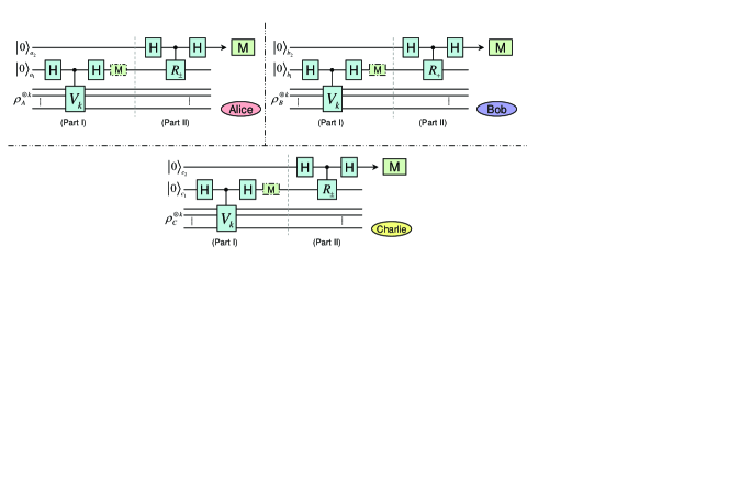
Figure 1: (Color online) A general network for remotely detecting the negativities in an unknown tripartite quantum state.

Now we analyze the first part of the LOCC network. This part is composed of three local modified interferometer circuits, in which the Hadamard gate and the controlled-$V_{k}$ gate can be represented by the unitary operators

$$H=\frac{1}{\sqrt{2}}\left(\begin{array}[]{cc}1&1\\ 1&-1\\ \end{array}\right),U_{C-V_{k}}=\left(\begin{array}[]{cc}1&0\\ 0&0\\ \end{array}\right)\otimes I+\left(\begin{array}[]{cc}0&0\\ 0&1\\ \end{array}\right)\otimes V_{k},$$ (14)

respectively. In this part, the input state is

$$\rho_{in}(k)=\rho_{ABC}^{\otimes k}\otimes\rho_{a_{1}b_{1}c_{1}},$$ (15)

where the quantum state $\rho_{a_{1}b_{1}c_{1}}=|000\rangle\langle 000|$ is the initial state of the ancillary qubits $a_{1}$, $b_{1}$ and $c_{1}$. After passing through the three interferometer circuits, the input state $\rho_{in}(k)$ will evolve into

$$\rho_{out}^{\prime}(k) = U_{h_{1}}U_{c-v}U_{h_{1}}\rho_{in}(k)U_{h_{1}}^{\dagger}U_{c-v}^{\dagger}U_{h_{1}}^{\dagger},$$ (16)

where $U_{h_{1}}=H_{a_{1}}\otimes H_{b_{1}}\otimes H_{c_{1}}\otimes I_{ABC}^{\otimes k}$ and $U_{c-v}=U_{C_{a_{1}}-V_{Ak}}\otimes U_{C_{b_{1}}-V_{Bk}}\otimes U_{C_{c_{1}}-V_{Ck}}$. In the output state, what we care about is the quantum state evolution of ancillary qubits $a_{1}$, $b_{1}$ and $c_{1}$. After tedious derivations, the output state of the ancillary qubits is found to be

$$\rho_{a_{1}b_{1}c_{1}}^{\prime}(k) = \mbox{Tr}_{ABC}[\rho_{out}^{\prime}(k)]$$ (25)

$$= \frac{1}{8}\left(\begin{array}[]{cccccccc}\mu_{1}^{(k)}&0&0&\mu_{9}^{(k)}&0&\mu_{10}^{(k)}&\mu_{11}^{(k)}&0\\ 0&\mu_{2}^{(k)}&-\mu_{9}^{(k)}&0&-\mu_{10}^{(k)}&0&0&\mu_{12}^{(k)}\\ 0&-\mu_{9}^{(k)}&\mu_{3}^{(k)}&0&-\mu_{11}^{(k)}&0&0&\mu_{13}^{(k)}\\ \mu_{9}^{(k)}&0&0&\mu_{4}^{(k)}&0&-\mu_{12}^{(k)}&-\mu_{13}^{(k)}&0\\ 0&-\mu_{10}^{(k)}&-\mu_{11}^{(k)}&0&\mu_{5}^{(k)}&0&0&\mu_{14}^{(k)}\\ \mu_{10}^{(k)}&0&0&-\mu_{12}^{(k)}&0&\mu_{6}^{(k)}&-\mu_{14}^{(k)}&0\\ \mu_{11}^{(k)}&0&0&-\mu_{13}^{(k)}&0&-\mu_{14}^{(k)}&\mu_{7}^{(k)}&0\\ 0&\mu_{12}^{(k)}&\mu_{13}^{(k)}&0&\mu_{14}^{(k)}&0&0&\mu_{8}^{(k)}\\ \end{array}\right),$$

where

$$\mu_{1}^{(k)} = 1+\alpha_{1}^{(k)}+\beta_{1}^{(k)}+\beta_{2}^{(k)}+\beta_{3}^{(k)}+\beta_{4}^{(k)}+\beta_{5}^{(k)}+\beta_{6}^{(k)}+\gamma_{1}^{(k)}+\gamma_{2}^{(k)}+\gamma_{3}^{(k)}+\gamma_{4}^{(k)},$$

$$\mu_{2}^{(k)} = 1+\alpha_{2}^{(k)}+\beta_{1}^{(k)}-\beta_{2}^{(k)}-\beta_{3}^{(k)}+\beta_{4}^{(k)}-\beta_{5}^{(k)}-\beta_{6}^{(k)}-\gamma_{1}^{(k)}-\gamma_{2}^{(k)}-\gamma_{3}^{(k)}-\gamma_{4}^{(k)},$$

$$\mu_{3}^{(k)} = 1+\alpha_{3}^{(k)}-\beta_{1}^{(k)}+\beta_{2}^{(k)}-\beta_{3}^{(k)}-\beta_{4}^{(k)}+\beta_{5}^{(k)}-\beta_{6}^{(k)}-\gamma_{1}^{(k)}-\gamma_{2}^{(k)}-\gamma_{3}^{(k)}-\gamma_{4}^{(k)},$$

$$\mu_{4}^{(k)} = 1+\alpha_{4}^{(k)}-\beta_{1}^{(k)}-\beta_{2}^{(k)}+\beta_{3}^{(k)}-\beta_{4}^{(k)}-\beta_{5}^{(k)}+\beta_{6}^{(k)}+\gamma_{1}^{(k)}+\gamma_{2}^{(k)}+\gamma_{3}^{(k)}+\gamma_{4}^{(k)},$$

$$\mu_{5}^{(k)} = 1-\alpha_{4}^{(k)}-\beta_{1}^{(k)}-\beta_{2}^{(k)}+\beta_{3}^{(k)}-\beta_{4}^{(k)}-\beta_{5}^{(k)}+\beta_{6}^{(k)}-\gamma_{1}^{(k)}-\gamma_{2}^{(k)}-\gamma_{3}^{(k)}-\gamma_{4}^{(k)},$$

$$\mu_{6}^{(k)} = 1-\alpha_{3}^{(k)}-\beta_{1}^{(k)}+\beta_{2}^{(k)}-\beta_{3}^{(k)}-\beta_{4}^{(k)}+\beta_{5}^{(k)}-\beta_{6}^{(k)}+\gamma_{1}^{(k)}+\gamma_{2}^{(k)}+\gamma_{3}^{(k)}+\gamma_{4}^{(k)},$$

$$\mu_{7}^{(k)} = 1-\alpha_{2}^{(k)}+\beta_{1}^{(k)}-\beta_{2}^{(k)}-\beta_{3}^{(k)}+\beta_{4}^{(k)}-\beta_{5}^{(k)}-\beta_{6}^{(k)}+\gamma_{1}^{(k)}+\gamma_{2}^{(k)}+\gamma_{3}^{(k)}+\gamma_{4}^{(k)},$$

$$\mu_{8}^{(k)} = 1-\alpha_{1}^{(k)}+\beta_{1}^{(k)}-\beta_{2}^{(k)}-\beta_{3}^{(k)}+\beta_{4}^{(k)}-\beta_{5}^{(k)}-\beta_{6}^{(k)}-\gamma_{1}^{(k)}-\gamma_{2}^{(k)}-\gamma_{3}^{(k)}-\gamma_{4}^{(k)},$$

$$\mu_{9}^{(k)} = \beta_{3}^{(k)}-\beta_{6}^{(k)}+\gamma_{1}^{(k)}+\gamma_{2}^{(k)}-\gamma_{3}^{(k)}-\gamma_{4}^{(k)},$$

$$\mu_{10}^{(k)} = \beta_{2}^{(k)}-\beta_{5}^{(k)}+\gamma_{1}^{(k)}-\gamma_{2}^{(k)}+\gamma_{3}^{(k)}-\gamma_{4}^{(k)},$$

$$\mu_{11}^{(k)} = \beta_{1}^{(k)}-\beta_{4}^{(k)}+\gamma_{1}^{(k)}-\gamma_{2}^{(k)}-\gamma_{3}^{(k)}+\gamma_{4}^{(k)},$$

$$\mu_{12}^{(k)} = \beta_{1}^{(k)}-\beta_{4}^{(k)}-\gamma_{1}^{(k)}+\gamma_{2}^{(k)}+\gamma_{3}^{(k)}-\gamma_{4}^{(k)},$$

$$\mu_{13}^{(k)} = \beta_{2}^{(k)}-\beta_{5}^{(k)}-\gamma_{1}^{(k)}+\gamma_{2}^{(k)}-\gamma_{3}^{(k)}+\gamma_{4}^{(k)},$$

$$\mu_{14}^{(k)} = \beta_{3}^{(k)}-\beta_{6}^{(k)}-\gamma_{1}^{(k)}-\gamma_{2}^{(k)}+\gamma_{3}^{(k)}+\gamma_{4}^{(k)},$$ (26)

in which

$$\alpha_{1}^{(k)} = \mbox{Tr}[V_{Ak}\rho_{A}^{\otimes k}]+\mbox{Tr}[V_{Bk}\rho_{B}^{\otimes k}]+\mbox{Tr}[V_{Ck}\rho_{C}^{\otimes k}]=\mbox{Tr}\rho_{A}^{k}+\mbox{Tr}\rho_{B}^{k}+\mbox{Tr}\rho_{C}^{k},$$

$$\alpha_{2}^{(k)} = \mbox{Tr}[V_{Ak}\rho_{A}^{\otimes k}]+\mbox{Tr}[V_{Bk}\rho_{B}^{\otimes k}]-\mbox{Tr}[V_{Ck}\rho_{C}^{\otimes k}]=\mbox{Tr}\rho_{A}^{k}+\mbox{Tr}\rho_{B}^{k}-\mbox{Tr}\rho_{C}^{k},$$

$$\alpha_{3}^{(k)} = \mbox{Tr}[V_{Ak}\rho_{A}^{\otimes k}]-\mbox{Tr}[V_{Bk}\rho_{B}^{\otimes k}]+\mbox{Tr}[V_{Ck}\rho_{C}^{\otimes k}]=\mbox{Tr}\rho_{A}^{k}-\mbox{Tr}\rho_{B}^{k}+\mbox{Tr}\rho_{C}^{k},$$

$$\alpha_{4}^{(k)} = \mbox{Tr}[V_{Ak}\rho_{A}^{\otimes k}]-\mbox{Tr}[V_{Bk}\rho_{B}^{\otimes k}]-\mbox{Tr}[V_{Ck}\rho_{C}^{\otimes k}]=\mbox{Tr}\rho_{A}^{k}-\mbox{Tr}\rho_{B}^{k}-\mbox{Tr}\rho_{C}^{k},$$

$$\beta_{1}^{(k)} = \frac{1}{2}\mbox{Tr}[(V_{Ak}\otimes V_{Bk})\rho_{AB}^{\otimes k}]=\frac{1}{2}\mbox{Tr}\rho_{AB}^{k},$$

$$\beta_{2}^{(k)} = \frac{1}{2}\mbox{Tr}[(V_{Ak}\otimes V_{Ck})\rho_{AC}^{\otimes k}]=\frac{1}{2}\mbox{Tr}\rho_{AC}^{k},$$

$$\beta_{3}^{(k)} = \frac{1}{2}\mbox{Tr}[(V_{Bk}\otimes V_{Ck})\rho_{BC}^{\otimes k}]=\frac{1}{2}\mbox{Tr}\rho_{BC}^{k},$$

$$\beta_{4}^{(k)} = \frac{1}{2}\mbox{Tr}[(V_{Ak}^{\dagger}\otimes V_{Bk})\rho_{AB}^{\otimes k}]=\frac{1}{2}\mbox{Tr}(\rho_{AB}^{T_{A}})^{k},$$

$$\beta_{5}^{(k)} = \frac{1}{2}\mbox{Tr}[(V_{Ak}^{\dagger}\otimes V_{Ck})\rho_{AC}^{\otimes k}]=\frac{1}{2}\mbox{Tr}(\rho_{AC}^{T_{A}})^{k},$$

$$\beta_{6}^{(k)} = \frac{1}{2}\mbox{Tr}([V_{Bk}^{\dagger}\otimes V_{Ck})\rho_{BC}^{\otimes k}]=\frac{1}{2}\mbox{Tr}(\rho_{BC}^{T_{B}})^{k},$$

$$\gamma_{1}^{(k)} = \frac{1}{4}\mbox{Tr}[(V_{Ak}\otimes V_{Bk}\otimes V_{Ck})\rho_{ABC}^{\otimes k}]=\frac{1}{4}\mbox{Tr}\rho_{ABC}^{k},$$

$$\gamma_{2}^{(k)} = \frac{1}{4}\mbox{Tr}[(V_{Ak}^{\dagger}\otimes V_{Bk}\otimes V_{Ck})\rho_{ABC}^{\otimes k}]=\frac{1}{4}\mbox{Tr}(\rho_{ABC}^{T_{A}})^{k},$$

$$\gamma_{3}^{(k)} = \frac{1}{4}\mbox{Tr}[(V_{Ak}\otimes V_{Bk}^{\dagger}\otimes V_{Ck})\rho_{ABC}^{\otimes k}]=\frac{1}{4}\mbox{Tr}(\rho_{ABC}^{T_{B}})^{k},$$

$$\gamma_{4}^{(k)} = \frac{1}{4}\mbox{Tr}[(V_{Ak}\otimes V_{Bk}\otimes V_{Ck}^{\dagger})\rho_{ABC}^{\otimes k}]=\frac{1}{4}\mbox{Tr}(\rho_{ABC}^{T_{C}})^{k}.$$ (27)

In the derivation of Eq. (25), we made use of the cyclicity of the trace and the property $\mbox{Tr}U^{\dagger}\rho=(\mbox{Tr}U\rho)^{\ast}$. In Eq. (II), the relations between the parameters $\alpha_{i}^{(k)}$, $\beta_{i}^{(k)}$, $\gamma_{i}^{(k)}$ and the traces of the corresponding matrices were analyzed in Ref. ekl02 ; aho03 ; car05 ; bla05 ; hab04 . In the first group of measurements, Alice, Bob and Charlie measure the expectation values of $\sigma_{z}\otimes\sigma_{z}\otimes\sigma_{z}$ on the output state $\rho_{a_{1}b_{1}c_{1}}^{\prime}(k)$, for $k=2,3,\cdots,d$. With these expectation values, they can get

$$\mbox{Tr}[(\sigma_{z}\otimes\sigma_{z}\otimes\sigma_{z})\rho_{a_{1}b_{1}c_{1}}^{\prime}(k)] = \gamma_{1}^{(k)}+\gamma_{2}^{(k)}+\gamma_{3}^{(k)}+\gamma_{4}^{(k)}$$ (28)

$$= \frac{1}{4}\mbox{Tr}\left(\rho_{ABC}^{k}+(\rho_{ABC}^{T_{A}})^{k}+(\rho_{ABC}^{T_{B}})^{k}+(\rho_{ABC}^{T_{C}})^{k}\right).$$

These expectation values can be obtained by collectively measuring the probabilities $P_{a_{1}b_{1}c_{1}}^{(k)}(ijl)$ of the output state $\rho_{a_{1}b_{1}c_{1}}^{\prime}(k)$ being found in the states $|000\rangle$,$|001\rangle$,$|010\rangle$,$|011\rangle$,$|100\rangle$,$|101\rangle$,$|110\rangle$ and $|111\rangle$, respectively, in which a classical communication is needed. With the probabilities $P_{a_{1}b_{1}c_{1}}^{(k)}(ijl)$, the three observers can also get the following relations:

$$\mbox{Tr}[(\sigma_{z}\otimes\sigma_{z})\rho_{a_{1}b_{1}}^{\prime}(k)] = \beta_{1}^{(k)}+\beta_{4}^{(k)}=\frac{1}{2}\left(\mbox{Tr}\rho_{AB}^{k}+\mbox{Tr}(\rho_{AB}^{T_{A}})^{k}\right)$$

$$\mbox{Tr}[(\sigma_{z}\otimes\sigma_{z})\rho_{a_{1}c_{1}}^{\prime}(k)] = \beta_{2}^{(k)}+\beta_{5}^{(k)}=\frac{1}{2}\left(\mbox{Tr}\rho_{AC}^{k}+\mbox{Tr}(\rho_{AC}^{T_{A}})^{k}\right)$$

$$\mbox{Tr}[(\sigma_{z}\otimes\sigma_{z})\rho_{b_{1}c_{1}}^{\prime}(k)] = \beta_{3}^{(k)}+\beta_{6}^{(k)}=\frac{1}{2}\left(\mbox{Tr}\rho_{BC}^{k}+\mbox{Tr}(\rho_{BC}^{T_{B}})^{k}\right),$$ (29)

where $\rho_{a_{1}b_{1}}^{\prime}(k)$, $\rho_{a_{1}c_{1}}^{\prime}(k)$ and $\rho_{b_{1}c_{1}}^{\prime}(k)$ are the bipartite reduced density matrices of $\rho_{a_{1}b_{1}c_{1}}^{\prime}(k)$. In Eqs. (10) and (11), the case for $k=2$ is special, which is due to the hermitian property of the shift operator $V_{2}$. Combining the hermitian property of $V_{2}$ and the definitions of $\beta_{i}$, $\gamma_{i}$, the three observers can have the following relations

$$\mbox{Tr}[(\sigma_{z}\otimes\sigma_{z}\otimes\sigma_{z})\rho_{a_{1}b_{1}c_{1}}^{\prime}(2)]=\mbox{Tr}\rho_{ABC}^{2}=\mbox{Tr}(\rho_{ABC}^{T_{A}})^{2}=\mbox{Tr}(\rho_{ABC}^{T_{B}})^{2}=\mbox{Tr}(\rho_{ABC}^{T_{C}})^{2}$$ (30)

$$\mbox{Tr}[(\sigma_{z}\otimes\sigma_{z})\rho_{a_{1}b_{1}}^{\prime}(2)]=\mbox{Tr}\rho_{AB}^{2}=\mbox{Tr}(\rho_{AB}^{T_{A}})^{2}$$

$$\mbox{Tr}[(\sigma_{z}\otimes\sigma_{z})\rho_{a_{1}c_{1}}^{\prime}(2)]=\mbox{Tr}\rho_{AC}^{2}=\mbox{Tr}(\rho_{AC}^{T_{A}})^{2}$$

$$\mbox{Tr}[(\sigma_{z}\otimes\sigma_{z})\rho_{b_{1}c_{1}}^{\prime}(2)]=\mbox{Tr}\rho_{BC}^{2}=\mbox{Tr}(\rho_{BC}^{T_{B}})^{2}.$$

While, for $k>2$, the shift operator $V_{k}$ is not hermitian pha03 , and the three observers cannot have the same relations as Eq. (30). From the above analysis, we can see that the three observers cannot obtain the requisite eigenvalues in general, unless the tripartite quantum state has the symmetrical property $\mbox{Tr}\rho_{ABC}^{k}=\mbox{Tr}(\rho_{ABC}^{T_{A}})^{k}=\mbox{Tr}(\rho_{ABC}^{T_{B}})^{k}=\mbox{Tr}(\rho_{ABC}^{T_{C}})^{k}$. This point seems to have been neglected in Ref. hab04 .

In order to obtain the eigenvalues of the set of partial transposition matrices for an arbitrary given tripartite quantum state, Alice, Bob and Charlie need to make other measurements. In the second group of measurements, they need to implement the whole LOCC network shown in Fig.1, in which they choose the controlled gates in the second part to be controlled-$R_{-}$, controlled-$R_{+}$ and controlled-$R_{+}$, respectively. In the second part, the input state is

$$\rho_{in}^{\prime}(k) = \rho^{\prime}_{a_{1}b_{1}c_{1}}(k)\otimes\rho_{a_{2}b_{2}c_{2}},$$ (31)

where the quantum state $\rho_{a_{2}b_{2}c_{2}}=|000\rangle\langle 000|$ is the initial state of the ancillary qubits $a_{2}$, $b_{2}$ and $c_{2}$. Passing through the three interferometer circuits, the input state $\rho_{in}^{\prime}(k)$ will evolve into the following form:

$$\rho_{out}^{-++}(k) = U_{h_{2}}U_{c-r_{1}}U_{h_{2}}\rho^{\prime}_{in}(k)U_{h_{2}}^{\dagger}U_{c-r_{1}}^{\dagger}U_{h_{2}}^{\dagger},$$ (32)

where $U_{h_{2}}=H_{a_{2}}\otimes H_{b_{2}}\otimes H_{c_{2}}\otimes I_{a_{1}b_{1}c_{1}}$ and $U_{c-r_{1}}=U_{C_{a_{2}}-R_{-}}\otimes U_{C_{b_{2}}-R_{+}}\otimes U_{C_{c_{2}}-R_{+}}$. In the output state $\rho_{out}^{-++}(k)$, what we care about is the quantum state evolution of the ancillary qubits $a_{2}$, $b_{2}$ and $c_{2}$. The corresponding output state is found to be

$$\rho_{a_{2}b_{2}c_{2}}^{-++}(k) = \mbox{Tr}_{a_{1}b_{1}c_{1}}[\rho_{out}^{-++}(k)]$$ (41)

$$= \frac{1}{8}\left(\begin{array}[]{cccccccc}\nu_{1}^{(k)}&0&0&0&0&0&0&0\\ 0&\nu_{2}^{(k)}&0&0&0&0&0&0\\ 0&0&\nu_{3}^{(k)}&0&0&0&0&0\\ 0&0&0&\nu_{4}^{(k)}&0&0&0&0\\ 0&0&0&0&\nu_{5}^{(k)}&0&0&0\\ 0&0&0&0&0&\nu_{6}^{(k)}&0&0\\ 0&0&0&0&0&0&\nu_{7}^{(k)}&0\\ 0&0&0&0&0&0&0&\nu_{8}^{(k)}\\ \end{array}\right),$$

where

$$\nu_{1}^{(k)} = 1+\frac{1}{\sqrt{2}}\alpha_{1}^{(k)}+\beta_{1}^{(k)}+\beta_{2}^{(k)}+\beta_{6}^{(k)}+\frac{1}{\sqrt{2}}\Gamma^{(k)},$$

$$\nu_{2}^{(k)} = 1+\frac{1}{\sqrt{2}}\alpha_{2}^{(k)}+\beta_{1}^{(k)}-\beta_{2}^{(k)}-\beta_{6}^{(k)}-\frac{1}{\sqrt{2}}\Gamma^{(k)},$$

$$\nu_{3}^{(k)} = 1+\frac{1}{\sqrt{2}}\alpha_{3}^{(k)}-\beta_{1}^{(k)}+\beta_{2}^{(k)}-\beta_{6}^{(k)}-\frac{1}{\sqrt{2}}\Gamma^{(k)},$$

$$\nu_{4}^{(k)} = 1+\frac{1}{\sqrt{2}}\alpha_{4}^{(k)}-\beta_{1}^{(k)}-\beta_{2}^{(k)}+\beta_{6}^{(k)}+\frac{1}{\sqrt{2}}\Gamma^{(k)},$$

$$\nu_{5}^{(k)} = 1-\frac{1}{\sqrt{2}}\alpha_{4}^{(k)}-\beta_{1}^{(k)}-\beta_{2}^{(k)}+\beta_{6}^{(k)}-\frac{1}{\sqrt{2}}\Gamma^{(k)},$$

$$\nu_{6}^{(k)} = 1-\frac{1}{\sqrt{2}}\alpha_{3}^{(k)}-\beta_{1}^{(k)}+\beta_{2}^{(k)}-\beta_{6}^{(k)}+\frac{1}{\sqrt{2}}\Gamma^{(k)},$$

$$\nu_{7}^{(k)} = 1-\frac{1}{\sqrt{2}}\alpha_{2}^{(k)}+\beta_{1}^{(k)}-\beta_{2}^{(k)}-\beta_{6}^{(k)}+\frac{1}{\sqrt{2}}\Gamma^{(k)},$$

$$\nu_{8}^{(k)} = 1-\frac{1}{\sqrt{2}}\alpha_{1}^{(k)}+\beta_{1}^{(k)}+\beta_{2}^{(k)}+\beta_{6}^{(k)}-\frac{1}{\sqrt{2}}\Gamma^{(k)},$$ (42)

in which $\Gamma^{(k)}=\gamma_{1}^{(k)}-\gamma_{2}^{(k)}+\gamma_{3}^{(k)}+\gamma_{4}^{(k)}$. In the second group of measurements, Alice, Bob and Charlie measure the expectation values of $\sigma_{z}\otimes\sigma_{z}\otimes\sigma_{z}$ on the output state $\rho_{a_{2}b_{2}c_{2}}^{-++}(k)$ for $k=3,4,\cdots,d$. These expectation values can be written as

$$\mbox{Tr}[(\sigma_{z}\otimes\sigma_{z}\otimes\sigma_{z})\rho_{a_{2}b_{2}c_{2}}^{-++}(k)] = \frac{1}{\sqrt{2}}(\gamma_{1}^{(k)}-\gamma_{2}^{(k)}+\gamma_{3}^{(k)}+\gamma_{4}^{(k)})$$ (43)

$$= \frac{1}{4\sqrt{2}}\mbox{Tr}\left[\rho_{ABC}^{k}-(\rho_{ABC}^{T_{A}})^{k}+(\rho_{ABC}^{T_{B}})^{k}+(\rho_{ABC}^{T_{C}})^{k}\right].$$

When they consider the expectation values of the bipartite reduced density matrices of $\rho_{a_{2}b_{2}c_{2}}^{-++}(k)$, they have

$$\mbox{Tr}[(\sigma_{z}\otimes\sigma_{z})\rho_{a_{2}b_{2}}^{-++}(k)] = \beta_{1}^{(k)}=\frac{1}{2}\mbox{Tr}\rho_{AB}^{k}$$

$$\mbox{Tr}[(\sigma_{z}\otimes\sigma_{z})\rho_{a_{2}c_{2}}^{-++}(k)] = \beta_{2}^{(k)}=\frac{1}{2}\mbox{Tr}\rho_{AC}^{k}$$

$$\mbox{Tr}[(\sigma_{z}\otimes\sigma_{z})\rho_{b_{2}c_{2}}^{-++}(k)] = \beta_{6}^{(k)}=\frac{1}{2}\mbox{Tr}(\rho_{BC}^{T_{B}})^{k}.$$ (44)

The expectation values in Eq. (43) and Eq. (II) can be obtain by measuring the probabilities $P_{a_{2}b_{2}c_{2}}^{(-++)(k)}(ijl)$ of the output state $\rho_{a_{2}b_{2}c_{2}}^{-++}(k)$ being found in the states $\{|ijl\rangle\}$.

In the third group of measurements, Alice, Bob and Charlie implement again the whole LOCC network. This time, they choose the controlled gates in the second part to be controlled-$R_{-}$, controlled-$R_{+}$ and controlled-$R_{-}$, respectively. The output state of the ancillary qubits $a_{2}$, $b_{2}$ and $c_{2}$ is

$$\rho_{a_{2}b_{2}c_{2}}^{-+-}(k)=\mbox{Tr}_{a_{1}b_{1}c_{1}}[\rho_{out}^{-+-}(k)] = \mbox{Tr}_{a_{1}b_{1}c_{1}}[U_{h_{2}}U_{c-r_{2}}U_{h_{2}}\rho^{\prime}_{in}(k)U_{h_{2}}^{\dagger}U_{c-r_{2}}^{\dagger}U_{h_{2}}^{\dagger}],$$ (45)

where $U_{c-r_{2}}=U_{C_{a_{2}}-R_{-}}\otimes U_{C_{b_{2}}-R_{+}}\otimes U_{C_{c_{2}}-R_{-}}$. By measuring the probabilities $P_{a_{2}b_{2}c_{2}}^{(-+-)(k)}(ijl)$ of the output state $\rho_{a_{2}b_{2}c_{2}}^{-+-}(k)$ being found in the states $\{|ijl\rangle\}$, they can obtain the following relations

$$\mbox{Tr}[(\sigma_{z}\otimes\sigma_{z}\otimes\sigma_{z})\rho_{a_{2}b_{2}c_{2}}^{-+-}(k)] = \frac{1}{\sqrt{2}}(\gamma_{1}^{(k)}+\gamma_{2}^{(k)}-\gamma_{3}^{(k)}+\gamma_{4}^{(k)})$$

$$= \frac{1}{4\sqrt{2}}\mbox{Tr}\left(\rho_{ABC}^{k}+(\rho_{ABC}^{T_{A}})^{k}-(\rho_{ABC}^{T_{B}})^{k}+(\rho_{ABC}^{T_{C}})^{k}\right),$$

$$\mbox{Tr}[(\sigma_{z}\otimes\sigma_{z})\rho_{a_{2}b_{2}}^{-+-}(k)] = \beta_{1}^{(k)}=\frac{1}{2}\mbox{Tr}\rho_{AB}^{k}$$

$$\mbox{Tr}[(\sigma_{z}\otimes\sigma_{z})\rho_{a_{2}c_{2}}^{-+-}(k)] = \beta_{5}^{(k)}=\frac{1}{2}\mbox{Tr}(\rho_{AC}^{k})^{T_{A}}$$

$$\mbox{Tr}[(\sigma_{z}\otimes\sigma_{z})\rho_{b_{2}c_{2}}^{-+-}(k)] = \beta_{3}^{(k)}=\frac{1}{2}\mbox{Tr}\rho_{BC}^{k},$$ (46)

where $k=3,4,\cdots,d$.

In the fourth group of measurements, the three observers still implement the whole LOCC network, but at this time they choose the controlled gates in the second part to be controlled-$R_{+}$, controlled-$R_{+}$ and controlled-$R_{-}$, respectively. The output state of the ancillary qubits $a_{2}$, $b_{2}$ and $c_{2}$ is

$$\rho_{a_{2}b_{2}c_{2}}^{++-}(k)=\mbox{Tr}_{a_{1}b_{1}c_{1}}[\rho_{out}^{++-}(k)] = \mbox{Tr}_{a_{1}b_{1}c_{1}}[U_{h_{2}}U_{c-r_{3}}U_{h_{2}}\rho^{\prime}_{in}(k)U_{h_{2}}^{\dagger}U_{c-r_{3}}^{\dagger}U_{h_{2}}^{\dagger}],$$ (47)

where $U_{c-r_{3}}=U_{C_{a_{2}}-R_{+}}\otimes U_{C_{b_{2}}-R_{+}}\otimes U_{C_{c_{2}}-R_{-}}$. By measuring the probabilities $P_{a_{2}b_{2}c_{2}}^{(++-)(k)}(ijl)$ of the output state $\rho_{a_{2}b_{2}c_{2}}^{++-}(k)$ being found in the states $\{|ijl\rangle\}$, Alice, Bob and Charlie have

$$\mbox{Tr}[(\sigma_{z}\otimes\sigma_{z}\otimes\sigma_{z})\rho_{a_{2}b_{2}c_{2}}^{++-}(k)] = \frac{1}{\sqrt{2}}(\gamma_{1}^{(k)}+\gamma_{2}^{(k)}+\gamma_{3}^{(k)}-\gamma_{4}^{(k)})$$

$$= \frac{1}{4\sqrt{2}}\mbox{Tr}\left(\rho_{ABC}^{k}+(\rho_{ABC}^{T_{A}})^{k}+(\rho_{ABC}^{T_{B}})^{k}-(\rho_{ABC}^{T_{C}})^{k}\right),$$

$$\mbox{Tr}[(\sigma_{z}\otimes\sigma_{z})\rho_{a_{2}b_{2}}^{++-}(k)] = \beta_{1}^{(k)}=\frac{1}{2}\mbox{Tr}(\rho_{AB}^{T_{A}})^{k}$$

$$\mbox{Tr}[(\sigma_{z}\otimes\sigma_{z})\rho_{a_{2}c_{2}}^{++-}(k)] = \beta_{5}^{(k)}=\frac{1}{2}\mbox{Tr}\rho_{AC}^{k}$$

$$\mbox{Tr}[(\sigma_{z}\otimes\sigma_{z})\rho_{b_{2}c_{2}}^{++-}(k)] = \beta_{3}^{(k)}=\frac{1}{2}\mbox{Tr}\rho_{BC}^{k},$$ (48)

where $k=3,4,\cdots,d$.

Once Alice, Bob and Charlie complete all the four groups of measurements, they can deduce the functions of the set of partial transposition matrices. According to Eqs. (II), (30), (43), (II), (II) and (II), they can get

$$\mbox{Tr}(\rho_{ABC}^{T_{A}})^{k}=2\mbox{Tr}[(\sigma_{z}\otimes\sigma_{z}\otimes\sigma_{z})\rho_{a_{1}b_{1}c_{1}}^{\prime}(k)]-2\sqrt{2}\mbox{Tr}[(\sigma_{z}\otimes\sigma_{z}\otimes\sigma_{z})\rho_{a_{2}b_{2}c_{2}}^{-++}(k)]$$

$$\mbox{Tr}(\rho_{ABC}^{T_{B}})^{k}=2\mbox{Tr}[(\sigma_{z}\otimes\sigma_{z}\otimes\sigma_{z})\rho_{a_{1}b_{1}c_{1}}^{\prime}(k)]-2\sqrt{2}\mbox{Tr}[(\sigma_{z}\otimes\sigma_{z}\otimes\sigma_{z})\rho_{a_{2}b_{2}c_{2}}^{-+-}(k)]$$

$$\mbox{Tr}(\rho_{ABC}^{T_{C}})^{k}=2\mbox{Tr}[(\sigma_{z}\otimes\sigma_{z}\otimes\sigma_{z})\rho_{a_{1}b_{1}c_{1}}^{\prime}(k)]-2\sqrt{2}\mbox{Tr}[(\sigma_{z}\otimes\sigma_{z}\otimes\sigma_{z})\rho_{a_{2}b_{2}c_{2}}^{++-}(k)]$$

$$\mbox{Tr}(\rho_{AB}^{T_{A}})^{k}=2\mbox{Tr}[(\sigma_{z}\otimes\sigma_{z})\rho_{a_{1}b_{1}}^{\prime}(k)]-2\mbox{Tr}[(\sigma_{z}\otimes\sigma_{z})\rho_{a_{2}b_{2}}^{-++}(k)]$$

$$\mbox{Tr}(\rho_{AC}^{T_{A}})^{k}=2\mbox{Tr}[(\sigma_{z}\otimes\sigma_{z})\rho_{a_{1}c_{1}}^{\prime}(k)]-2\mbox{Tr}[(\sigma_{z}\otimes\sigma_{z})\rho_{a_{2}c_{2}}^{-++}(k)]$$

$$\mbox{Tr}(\rho_{BC}^{T_{B}})^{k}=2\mbox{Tr}[(\sigma_{z}\otimes\sigma_{z})\rho_{a_{2}c_{2}}^{-++}(k)],$$ (49)

where $k=3,4,\cdots,d$. Combining the above equation with Eq. (30), they can determine the requisite eigenvalues and then the set of negativites $\mathcal{N}_{(A-BC)}$, $\mathcal{N}_{(B-AC)}$, $\mathcal{N}_{(C-AB)}$, $\mathcal{N}_{(A-B)}$, $\mathcal{N}_{(A-C)}$ and $\mathcal{N}_{(B-C)}$.

III discussions

Our LOCC direct method is more parametrically efficient than the LOCC quantum state tomography. For a $d$-dimensional tripartite quantum state $\rho_{ABC}$, the quantum state tomography needs to measure $d^{2}-1$ parameters. However, our direct method merely requires to measure $4(d-2)+1$ parameters. Figure 2 shows the number of parameters that need to be measured in quantum state tomography (square) and our direct method (triangle) for the $2\otimes 2\otimes 2$, $2\otimes 2\otimes 3$, $2\otimes 2\otimes 4$ and $2\otimes 3\otimes 3$ quantum states.

Figure 2: The number of required parameters in the LOCC quantum state tomography (square) and our LOCC direct method (triangle) for some lower dimensional tripartite quantum states.

In one-to-two party quantum communication, the observers possibly care only about a part of the set of negativities. For example, in the communication of Alice to Bob and Charlie, they only want to know the negativities $\mathcal{N}_{(A-BC)}$, $\mathcal{N}_{(A-B)}$ and $\mathcal{N}_{(A-C)}$. In this case, the three observers need only to make the first and the second group of measurements, i.e., to measure $2d-3$ parameters. Then, by comparing the tripartite relations and bipartite relations in Eqs. (28), (II), (43) and (II), they can obtain the target negativities. Similarly, if they measure the first and third group of parameters (or the first and forth group of parameters), they can obtain $\{\mathcal{N}_{(B-AC)},\mathcal{N}_{(A-B)},\mathcal{N}_{(B-C)}\}$ (or $\{\mathcal{N}_{(C-AB)},\mathcal{N}_{(A-C)},\mathcal{N}_{(B-C)}\}$) in terms of corresponding relations.

As is known, the majorization criterion nak01 is stronger than the entropic inequality. The criterion states that if $\rho_{AB}$ is separable then $\lambda(\rho_{AB})\prec\lambda(\rho_{A})$ and $\lambda(\rho_{AB})\prec\lambda(\rho_{B})$, where $\lambda(\rho)$ is the eigenvalue vector of $\rho$. The relation $x\prec y$ between two n-dimensional vectors means that $\sum_{i=1}^{k}x_{i}^{\downarrow}\leq\sum_{i=1}^{k}y_{i}^{\downarrow},(1\leq k\leq n-1)$ and $\sum_{i=1}^{n}x_{i}^{\downarrow}=\sum_{i=1}^{n}y_{i}^{\downarrow}$, in which the symbol “$\downarrow$” stands for the decreasing order of the components of the vector. If the dimensions of $x$ and $y$ are different, the smaller vector is enlarged by appending extra zeros to equalize their dimensions. In the tripartite system, Alice, Bob and Charlie may characterize the entanglement in terms of a set of majorization criteria related to the eigenvalue vectors $\lambda(\rho_{ABC})$, $\lambda(\rho_{AB})$, $\lambda(\rho_{AC})$, $\lambda(\rho_{BC})$, $\lambda(\rho_{A})$, $\lambda(\rho_{B})$ and $\lambda(\rho_{C})$. In order to testing the set of criteria, they need to perform two groups of measurements, in which $2d-3$ parameters are measured. In the first group, they implement the first part of the LOCC network shown in Fig.1 and then measure the probabilities $P_{a_{1}b_{1}c_{1}}^{(k)}(ijl)$ for $k=2,3,\cdots,d$. In the second group, they implement the whole LOCC network in which all the controlled gates in the second part are chosen to be controlled-$R_{+}$, and then measure the probabilities $\rho_{a_{2}b_{2}c_{2}}^{+++}(k)$ for $k=3,4,\cdots,d$. After completing these measurements, they can get two groups of relations, by which they can obtain the target eigenvalue vectors.

However, in general, the majorization criterion is weaker than the PPT criterion. Alice, Bob and Charlie can use a set of PPT criteria to detect some bound entangled states which cannot be detected by the corresponding majorization criteria. The Dür-Cirac-Tarrach (DCT) state is just such a kind of quantum state, which takes the form dct99

$$\rho_{DCT} = \sum_{\sigma=\pm}\lambda_{0}^{\sigma}|\Psi_{0}^{\sigma}\rangle\langle\Psi_{0}^{\sigma}|+\sum_{k=01,10,11}\lambda_{k}(|\Psi_{k}^{+}\rangle\langle\Psi_{k}^{+}|+|\Psi_{k}^{+}\rangle\langle\Psi_{k}^{+}|),$$ (50)

where $|\Psi_{k}^{\pm}\rangle=(|k_{1}k_{2}0\rangle\pm|\overline{k}_{1}\overline{k}_{2}1\rangle)/\sqrt{2}$, with $k_{1}$ and $k_{2}$ as the binary digits of $k$ and $\overline{k}_{i}$ as the flipped $k_{i}$. When the parameters are chosen to be $\lambda_{0}^{+}=\frac{1}{3}$, $\lambda_{0}^{-}=\lambda_{10}=0$ and $\lambda_{01}=\lambda_{11}=\frac{1}{6}$, the corresponding quantum state is a bound entangled state and its matrix form reads

$$\rho_{bound}=\left(\begin{array}[]{cccccccc}\frac{1}{6}&0&0&0&0&0&0&\frac{1}{6}\\ 0&\frac{1}{6}&0&0&0&0&0&0\\ 0&0&\frac{1}{6}&0&0&0&0&0\\ 0&0&0&0&0&0&0&0\\ 0&0&0&0&0&0&0&0\\ 0&0&0&0&0&\frac{1}{6}&0&0\\ 0&0&0&0&0&0&\frac{1}{6}&0\\ \frac{1}{6}&0&0&0&0&0&0&\frac{1}{6}\\ \end{array}\right)$$ (59)

in the computational basis $\{|ijl\rangle\}$. The method for generating and detecting the DCT bound entanglement was given by Hyllus et al. hab04 . Here, we redescribe the detection procedure with our LOCC direct method. It is assumed that Alice, Bob and Charlie share a number of copies of quantum state $\rho_{bound}$ which is unknown to the three observers. After performing the four groups of measurements with the network shown in Fig.1, they can obtain theoretically the data listed in Table 1.

$\begin{array}[]{cc}&k\\ <\sigma_{z}^{\otimes 3}>_{(k)}&\\ \end{array}$	2	3	4	5	6	7	8
$<\sigma_{z}^{\otimes 3}>_{(k)}^{a_{1}b_{1}c_{1}}$	$\frac{2}{9}$	$\frac{7}{144}$	$\frac{17}{1296}$	$\frac{19}{5284}$	$\frac{51}{46656}$	$\frac{67}{186624}$	$\frac{197}{1679616}$
$<\sigma_{z}^{\otimes 3}>_{(k)}^{-++}$	/	$\frac{5}{144\sqrt{2}}$	$\frac{13}{1296\sqrt{2}}$	$\frac{17}{5184\sqrt{2}}$	$\frac{49}{46656\sqrt{2}}$	$\frac{65}{186624\sqrt{2}}$	$\frac{193}{1679616\sqrt{2}}$
$<\sigma_{z}^{\otimes 3}>_{(k)}^{-+-}$	/	$\frac{1}{48\sqrt{2}}$	$\frac{7}{1296\sqrt{2}}$	$\frac{7}{5184\sqrt{2}}$	$\frac{19}{46656\sqrt{2}}$	$\frac{23}{186624\sqrt{2}}$	$\frac{67}{1679616\sqrt{2}}$
$<\sigma_{z}^{\otimes 3}>_{(k)}^{++-}$	/	$\frac{1}{48\sqrt{2}}$	$\frac{7}{1296\sqrt{2}}$	$\frac{7}{5184\sqrt{2}}$	$\frac{19}{46656\sqrt{2}}$	$\frac{23}{186624\sqrt{2}}$	$\frac{67}{1679616\sqrt{2}}$

Table 1: Theoretical values of the four groups of parameters for the quantum state $\rho_{bound}$ in our LOCC direct method.

Combining these data with Eq. (II), the three observers can deduce that $\rho_{bound}^{T_{A}}$ is negative and other partial transposition matrices is semi-positive. Based on the negative eigenvalue, they can obtain further the $\mathcal{N}_{A-BC}(\rho_{bound})=\frac{1}{6}$. Here, it is noted that only when an infinite ensemble of identically prepared output state is given can Alice, Bob and Charlie determine the parameter precisely. When a finite ensemble is given, they can only determine the parameter approximately. Therefore, in order to obtain these parameters with high fidelity, they need to run the network many times. Especially, for $k$ is bigger, they need to implement the network even more times.

Although our method that makes use of bipartite entanglement measures is limited to characterize partially the tripartite quantum state, it can occasionally detect the genuine tripartite entanglement in some specific cases. For example, in the case of three-qubit quantum state, when $\mathcal{N}_{AB}=0$, $\mathcal{N}_{AC}=0$ and $\mathcal{N}_{A-BC}>0$, we can deduce that the entanglement in the bipartite splitting $A-BC$ is actually the genuine tripartite entanglement among Alice, Bob and Charlie. This is because that the negativities $\mathcal{N}_{AB}$ and $\mathcal{N}_{AC}$ can characterize the two-qubit entanglement sufficiently. When the two entanglements are zero, the residual entanglement $\mathcal{N}_{A-BC}$ must be the tripartite entanglement. The quantum state $\rho_{bound}$ in Eq. (25) is just the case. Similarly, when $\mathcal{N}_{AB}=0,\mathcal{N}_{BC}=0$ and $\mathcal{N}_{B-AC}>0$ (or $\mathcal{N}_{AC}=0,\mathcal{N}_{BC}=0$ and $\mathcal{N}_{C-AB}>0$), we are also able to judge that $\mathcal{N}_{B-AC}$ (or $\mathcal{N}_{C-AB}$) is of tripartite entanglement. Certainly, for a general three-qubit mixed state, whether or not the tripartite entanglement exists cannot be detected, simply because a well-defined tripartite entanglement measure is still unavailable, though a lot of efforts have been made.

Two problems are worth to remark in our LOCC method. First, the set of negativities can only quantify some aspects of the entanglement in a tripartite system. There exists some tripartite entangled state abl01 that is PPT with respect to any of the bipartite splitting. Moreover, as pointed by Hyluss et al. hab04 , there is a potential problem in practical application of the direct methods, i.e., how to implement effectively the controlled quantum gates, especially the controlled-swap gate hfc95 . The solution of this problem relies on the quantum technology that is currently being developed.

IV conclusions

In this paper, we have generalized the direct approach of Hyllus et al. hab04 and proposed an LOCC method for detecting a set of negativities in an arbitrary given tripartite quantum state. The main task for the three observers is to measure $4(d-2)+1$ parameters via three local networks supplemented by a classical communication. Comparing with the LOCC quantum state tomography which requires to measure $d^{2}-1$ parameters, our LOCC method is more efficient. Moreover, our LOCC method does not require the observers to perform the SPA of partial transposition maps, which supports the Carteret’s opinion car05 on the three-party scenario, i.e., it is not the only way that they make the quantum state undergo the partial transposition map, if Alice, Bob and Charlie want to measure the function of the partial transposition of $\rho_{ABC}$.

References

• (1) A. Einstein, B. Podolsky, and N. Rosen, Phys. Rev. 47, 777 (1935).
• (2) C. H. Bennett, G. Brassard, C. Crépeau, R. Jozsa, A. Peres, and W. K. Wootters, Phys. Rev. Lett. 70, 1895 (1993).
• (3) A. K. Ekert, Phys. Rev. Lett. 67, 661 (1991).
• (4) C. H. Bennett and S. Wiesner, Phys. Rev. Lett. 69, 2881 (1992).
• (5) K. Vogel, H. Risken, Phys. Rev. A 40, R2847 (1989).
• (6) D. T. Smithey, M. Beck, M. G. Raymer and A. Faradani, Phys. Rev. Lett. 70, 1244 (1993).
• (7) K. J. Resch, P. Walther, and A. Zeilinger, Phys. Rev. Lett. 94, 070402 (2005).
• (8) J. T. Barreiro, N. K. Langford, N. A. Peters, and P. G. Kwiat, Phys. Rev. Lett. 95, 260501 (2005).
• (9) P. Horodecki and A. Ekert, Phys. Rev. Lett. 89, 127902 (2002).
• (10) P. Horodecki, Phys. Rev. Lett. 90, 167901 (2003).
• (11) A. Peres, Phys. Rev. Lett. 77, 1413 (1996)
• (12) M. Horodecki, P. Horodecki, and R. Horodecki, Phys. Lett. A 223, 1 (1996).
• (13) P. Horodecki, Phys. Rev. A 68, 052101 (2003).
• (14) E. Sjöqvist, A. K. Pati, A. Ekert, J. S. Anandan, M. Ericsson, D. K. L. Oi, and V. Vedral, Phys. Rev. Lett. 85, 2845 (2000).
• (15) A. K. Ekert, C. M. Alves, D. K. L. Oi, M. Horodecki, P. Horodecki, and L. C. Kwek, Phys. Rev. Lett. 88, 217901 (2002).
• (16) H. A. Carteret, Phys. Rev. Lett. 94, 040502, (2005).
• (17) H. A. Carteret, quant-ph/0309212v6.
• (18) C. M. Alves and D. Jaksch, Phys. Rev. Lett. 93, 110501 (2004).
• (19) R. N. Palmer, C. M. Alves, and D. Jaksch, Phys. Rev. A 72, 042335 (2005).
• (20) M. Curty, M. Lewenstein and N. Lütkenhaus, Phys. Rev. Lett. 92, 217903 (2004).
• (21) C. M. Alves, P. Horodecki, D. K. L. Oi, L. C. Kwek, and A. K. Ekert, Phys. Rev. A 68, 032306 (2003).
• (22) Y.-K. Bai, S.-S. Li and H.-Z. Zheng, J. Phys. A 38, 8633 (2005).
• (23) Y.-K. Bai, S.-S. Li and H.-Z. Zheng, Phys. Rev. A 72, 052320 (2005).
• (24) R. Cleve, D. Gottesman, and H.-K. Lo, Phys. Rev. Lett. 83, 648 (1999).
• (25) A. Cabello, Phys. Rev. Lett. 89, 100402 (2002).
• (26) Y.-A. Chen, A.-N. Zhang, Z. Zhao, X.-Q. Zhou, C.-Y. Lu, C.-Z. Peng, T. Yang, and J.-W. Pan, Phys. Rev. Lett. 95, 200502 (2005).
• (27) G. Vidal and R. F. Werner, Phys. Rev. A 65, 032314 (2002)
• (28) P. Hyllus, C. M. Alves, D. Bruß, and C. Macchiavello, Phys. Rev. A 70, 032316 (2004)
• (29) W. Dür, J. I. Cirac, and R. Tarrach, Phys. Rev. Lett. 83, 3562 (1999).
• (30) M. A. Nielsen and J. Kempe, Phys. Rev. Lett. 86, 5184 (2001).
• (31) A. Acin, D. Bruß, M. Lewenstein, and A. Sanpera, Phys. Rev. Lett. 87, 040401 (2001).
• (32) H. F. Chau and F. Wilczek, Phys. Rev. Lett. 75, 748 (1995).