The characteristic function and entanglement of optical evolution

Abstract

The master equation of quantum optical density operator is transformed to the equation of characteristic function. The parametric amplification and amplitude damping as well as the phase damping are considered. The solution for the most general initial quantum state is obtained for parametric amplification and amplitude damping. The purity of one mode Gaussian system and the entanglement of two mode Gaussian system are studied.

PACS: 03.65.Yz ; 42.50.Dv; 42.50.Lc

Keywords: parametric amplifier, amplitude damping, phase damping, characteristic function

1 Introduction

Quantum information with continuous variables (CV) [1] [2] is a flourishing field, as shown by the spectacular implementations of deterministic teleportation schemes[3] [4] [5] [6], quantum key distribution protocols [7], entanglement swapping [5] [8], dense coding [9], quantum state storage [10] and quantum computation [11] processes in quantum optical settings . The crucial resource enabling a better-than-classical manipulation and processing of information is CV entanglement. In all such practical instances the information and entanglement contained in a given quantum state of the system, so precious for the realization of any specific task, is constantly threatened by the unavoidable interaction with the environment. Such an interaction entangles the system of interest with the environment, causing some amount of information to be scattered and lost in the environment. The overall process, corresponding to a non unitary evolution of the system, is commonly referred to as decoherence [4] [5]. In this work we study the decoherences of general states of continuous variable systems whose evolutions are ruled by optical master equations. We will consider the parametric amplification, amplitude damping and phase damping [12] of a general quantum CV state in the fashion of quantum characteristic function. The main starting point for this research work was the result of Lindblad’s bounded generator of a completely positive quantum dynamical semigroup [13]. Quantum characteristic function had been used to treat the amplitude damping of one mode squeezed states [14].

2 Time evolution of characteristic function

The density matrix obeys the following master equation [12] [13][15]

$$\frac{d\rho}{dt}=-\frac{i}{\hbar}[H,\rho]+(\mathcal{L}_{1}\mathcal{+L}_{2})\rho.$$ (1)

with the quadratic Hamiltonian

$$H=\hbar\sum_{jk}\frac{i}{2}(\eta_{jk}a_{j}^{\dagger}a_{k}^{\dagger}-\eta_{jk}^{*}a_{j}a_{k})$$ (2)

where $\eta$ is a complex symmetric matrix. In the single-mode case, this Hamiltonian describes two-photon downconversion from an undepleted (classical) pump[15]. The full multi-mode model describes quasi-particle excitation in a BEC within the Bogoliubov approximation [16]. This item represents the parametric amplifier. While the amplitude damping is described by $\mathcal{L}_{1},$

$$\mathcal{L}_{1}\rho = \sum_{j}\frac{\Gamma_{j}}{2}\{(\overline{n}_{j}+1)L[a_{j}]\rho+\overline{n}_{j}L[a_{j}^{\dagger}]\rho$$

$$-w_{j}^{*}M[a_{j}]\rho-w_{j}M[a_{j}^{\dagger}]\rho\}.$$

where the Lindblad super-operators are defined as $L[\widehat{o}]\rho\equiv$ $2\widehat{o}\rho\widehat{o}^{\dagger}-\widehat{o}^{\dagger}\widehat{o}\rho-\rho\widehat{o}^{\dagger}\widehat{o}$ and $M[\widehat{o}]\rho\equiv 2\widehat{o}\rho\widehat{o}-\widehat{o}\widehat{o}\rho-\rho\widehat{o}\widehat{o}.$ The requirement of positivity of the density operator imposes the constraint $\left|w_{j}\right|^{2}\leq\overline{n}_{j}(\overline{n}_{j}+1).$ At thermal equilibrium, i.e. $w_{j}=0,$ $\overline{n}_{j}$ is equal to the average thermal photon number of the environment. If $w_{j}\neq 0,$ then the bath $j$ is said to be ‘squeezed’[17].

$\mathcal{L}_{2}$ describes the phase damping,

$$\mathcal{L}_{2}\rho=\sum_{j}\frac{\gamma_{j}}{2}L[a_{j}^{\dagger}a_{j}]\rho.$$ (4)

We now transform the density operator master equation to the diffusion equation of the characteristic function. We use characteristic function because it is more convinent for our problem. One may use Glauber’s P-representation instead, but Glauber’s P-representation does not exist for some of the states (e.g.[14] [18]), although the generalised positive P-representation does always exist [19]. Any quantum state can be equivalently specified by its characteristic function. Every operator $\mathcal{A}\in\mathcal{B(H)}$ is completely determined by its characteristic function $\chi_{\mathcal{A}}:=tr[\mathcal{AD}(\mu)]$ [20], where $\mathcal{D}(\mu)=\exp(\mu a^{\dagger}-\mu^{*}a)$ is the displacement operator, with $\mu=[\mu_{1},\mu_{2},\cdots,\mu_{s}]$ $,a=[a_{1},a_{2},\cdots,a_{s}]^{T}$ and the total number of modes is $s.$ It follows that $\mathcal{A}$ may be written in terms of $\chi_{\mathcal{A}}$ as [21]: $\mathcal{A}=\int[\prod_{i}\frac{d^{2}\mu_{i}}{\pi}]\chi_{\mathcal{A}}(\mu)\mathcal{D}(-\mu).$ The density matrix $\rho$ can be expressed with its characteristic function $\chi$. $\chi=tr[\rho\mathcal{D}(\mu)]$ . Multiplying $\mathcal{D}(\mu)$ to the master equation then taking trace, the master equation of density operator will be transformed to the diffusion eqation of the characteristic function. It should be noted that the complex parameters $\mu_{j}$ are not a function of time, thus $\frac{\partial\chi}{\partial t}=tr[\frac{\partial\rho}{\partial t}\mathcal{D}(\mu)],$ the parametric amplification part in the form of characteristic function will be [15]

$$\frac{1}{2}tr\{\sum_{jk}[\eta_{jk}a_{j}^{\dagger}a_{k}^{\dagger}-\eta_{jk}^{*}a_{j}a_{k},\rho]D(\mu)\}=-\sum_{jk}(\eta_{jk}\mu_{j}^{*}\frac{\partial\chi}{\partial\mu_{k}}+\eta_{jk}^{*}\mu_{j}\frac{\partial\chi}{\partial\mu_{k}^{*}}).$$ (5)

The master equation can be transformed to the diffusion equation of the characteristic function, it is

$$\frac{\partial\chi}{\partial t} = -\sum_{jk}(\eta_{jk}\mu_{j}^{*}\frac{\partial\chi}{\partial\mu_{k}}+\eta_{jk}^{*}\mu_{j}\frac{\partial\chi}{\partial\mu_{k}^{*}})$$

$$-\frac{1}{2}\sum_{j}\Gamma_{j}\{\left|\mu_{j}\right|\frac{\partial\chi}{\partial\left|\mu_{j}\right|}+((2\overline{n}_{j}+1)\left|\mu_{j}\right|^{2}-w_{j}^{*}\mu_{j}^{2}-w_{j}\mu_{j}^{*2})\chi\}$$

$$+\frac{1}{2}\sum_{j}\gamma_{j}\frac{\partial^{2}\chi}{\partial\theta_{j}^{2}}.$$

Where we denote $\mu_{j}$ as $\left|\mu_{j}\right|e^{i\theta_{j}},$ and we should take care about that the variables are $\mu_{j}$ and $\mu_{j}^{*}$ in the amplification while they are $\left|\mu_{j}\right|$ $,\theta_{j}$ in the damping.

3 Solutions of some special cases

Firstly, let us consider $\Gamma_{j}=\gamma_{j}=0$ for all $j,$ the solution to the amplification is

$$\chi(\mu,\mu^{*},t)=\chi(\nu,\nu^{*},0),$$ (7)

with

$$(\nu,\nu^{*})=(\mu,\mu^{*})\left(\begin{array}[]{ll}\cosh^{*}(\left|\eta\right|t)&-\eta^{*}\frac{\sinh(\left|\eta\right|t)}{\left|\eta\right|}\\ -\frac{\sinh(\left|\eta\right|t)}{\left|\eta\right|}\eta&\cosh(\left|\eta\right|t)\end{array}\right),$$ (8)

where the matrix cosh and sinh functions are defined as[22]

$$\cosh\left|\xi\right| = I+\frac{1}{2!}\xi\xi^{*}+\frac{1}{4!}(\xi\xi^{*})^{2}+\cdots,$$ (9)

$$\frac{\sinh\left|\xi\right|}{\left|\xi\right|}\xi = \xi+\frac{1}{3!}\xi\xi^{*}\xi+\frac{1}{5!}(\xi\xi^{*})^{2}\xi+\cdots.$$

Then suppose $\eta=0$ and $\gamma_{j}=0$ for all $j,$ the solution to the amplitude damping equation of $\chi$ is

$$\chi(\mu,t)=\chi(\mu e^{-\frac{\Gamma t}{2}},0)\exp\{-\sum_{j}(1-e^{-\Gamma_{j}t})[(\overline{n}_{j}+\frac{1}{2})\left|\mu_{j}\right|^{2}-\frac{1}{2}w_{j}^{*}\mu_{j}^{2}-\frac{1}{2}w_{j}\mu_{j}^{*2}]\}.$$ (10)

Where $\mu e^{-\frac{\Gamma t}{2}}$ is the abbreviation of $(\mu_{1}e^{-\frac{\Gamma_{1}t}{2}},\mu_{2}e^{-\frac{\Gamma_{2}t}{2}},\cdots,\mu_{s}e^{-\frac{\Gamma_{s}t}{2}})$. Next, suppose $\eta=0$ and $\Gamma_{j}=0$ for all $j,$ the solution to the phase equation of $\chi$ then will be

$$\chi(\mu,\mu^{*},t)=\int dx\chi(\mu e^{ix},\mu^{*}e^{-ix},0)\prod_{i}(2\pi\gamma_{i}t)^{-1/2}\exp(-\frac{x_{i}^{2}}{2\gamma_{i}t}),$$ (11)

where $\mu e^{ix}$ is the abbreviation of $(\mu_{1}e^{ix_{1}},\mu_{2}e^{ix_{2}},\cdots,\mu_{s}e^{ix_{s}})$. The simultaneous amplitude and phase damping ($\eta=0$) for any initial characteristic function is (for $w_{j}=0$) [23]

$$\chi(\mu,\mu^{*},t) = \int dx\chi(\mu e^{-\frac{\Gamma t}{2}+ix},\mu^{*}e^{-\frac{\Gamma t}{2}-ix},0)\prod_{j}(2\pi\gamma_{j}t)^{-1/2}$$

$$\exp[-\frac{x_{j}^{2}}{2\gamma_{j}t}-(1-e^{-\Gamma_{i}t})(\overline{n}_{j}+\frac{1}{2})\left|\mu_{j}\right|^{2}].$$

The density matrix then can be obtained by making use of operator integral.

4 The parametric amplifier and the amplitude damping

The diffusion equation (2) now is with its $\gamma_{j}=0$ for all $j$. Suppose the solution to the diffusion equation is

$$\chi(\mu,\mu^{*},t)=\chi(\nu,\nu^{*},0)\exp[\frac{1}{2}(\nu,-\nu^{*})\left(\begin{array}[]{ll}\alpha&\beta^{*}\\ \beta&\alpha^{*}\end{array}\right)(\nu^{*},-\nu)^{T}-\frac{1}{2}(\mu,-\mu^{*})\left(\begin{array}[]{ll}\alpha&\beta^{*}\\ \beta&\alpha^{*}\end{array}\right)(\mu^{*},-\mu)^{T}],$$ (13)

where $\nu=\mu M+\mu^{*}N,$ with $M$ and $N$ being time varying matrices. $\alpha$ and $\beta$ are constant matrices and $\alpha^{\dagger}=\alpha,$ $\beta=\beta^{T}$. $M$ and $N$ are the solutions of the following matrix equations

$$\frac{dM}{dt} = -\eta^{*}N-\frac{\Gamma}{2}M,$$ (14)

$$\frac{dN}{dt} = -\eta M-\frac{\Gamma}{2}N,$$ (15)

where $\Gamma=diag\{\Gamma_{1},\Gamma_{2},\cdots,\Gamma_{s}\}.$ While $\alpha$ and $\beta$ are the solution of the following matrix equations

$$2\eta\alpha+2\alpha^{*}\eta-\Gamma\beta-\beta\Gamma+\Gamma w+w\Gamma = 0,$$ (16)

$$\Gamma\alpha+\alpha\Gamma-2\eta^{*}\beta-2\beta^{*}\eta-\Gamma(\overline{n}+\frac{1}{2})-(\overline{n}+\frac{1}{2})\Gamma = 0.$$ (17)

where $w$ $=diag\{w_{1},w_{2},\cdots,w_{s}\},\overline{n}=diag\{\overline{n}_{1},\overline{n}_{2},\cdots,\overline{n}_{s}\}.$ The constant matrices $\alpha$ and $\beta$ can be worked out as the solution of linear algebraic equations (16) and (17). What left is to solve matrix equations (14) and (15). There are two situations that the equations are solvable. The first case is that all the modes undergo the same amplitude damping, that is $\Gamma_{1}=\Gamma_{2}=\cdots=\Gamma_{s}$, thus $\Gamma=\Gamma_{1}\mathbf{I}_{s}.$ $\Gamma$ commutes with any matrix. Equations (14) and (15) have solution

$$M = e^{-\frac{1}{2}\Gamma t}\cosh^{*}(\left|\eta\right|t),$$ (18)

$$N = -e^{-\frac{1}{2}\Gamma t}\frac{\sinh(\left|\eta\right|t)}{\left|\eta\right|}\eta.$$ (19)

The solution to the one-mode situation is simple. In the two-mode situation, $M$ and $N$ can be further simplified. For $\eta$ is a symmetric matrix, we can express it as $\eta=\eta_{0}\sigma_{0}+\eta_{1}\sigma_{1}+\eta_{3}\sigma_{3},$ where $\sigma_{0}=\mathbf{I}_{2},$ $\sigma_{i}$ $(i=1,2,3)$ are Pauli matrices. The $\sigma_{2}$ term is nulled by the symmetry of $\eta.$ By using of the algebra of Pauli matrices, we arrive at the results:

$$\cosh(\left|\eta\right|t) = \sigma_{0}\cosh(\sqrt{(C+A)/2}t)\cosh(\sqrt{(C-A)/2}t)$$

$$+\sinh(\sqrt{(C+A)/2}t)\sinh(\sqrt{(C-A)/2}t)\overrightarrow{\sigma}\cdot\overrightarrow{b},$$

$$\frac{\sinh(\left|\eta\right|t)}{\left|\eta\right|}\eta = \frac{1}{2}\sigma_{0}[\sinh(\sqrt{(C+B)}t)/\sqrt{(C+B)}+\sinh(\sqrt{(C-B)}t)/\sqrt{(C-B)}]\eta$$

$$+\frac{1}{2}[\sinh(\sqrt{(C+B)}t)/\sqrt{(C+B)}-\sinh(\sqrt{(C-B)}t)/\sqrt{(C-B)}]\overrightarrow{\sigma}\cdot\overrightarrow{b}\eta.$$

Where $C=\left|\eta_{0}\right|^{2}+\left|\eta_{1}\right|^{2}+\left|\eta_{3}\right|^{2},$ $A=\left|\eta_{0}^{2}-\eta_{1}^{2}-\eta_{3}^{2}\right|,$ $B=\sqrt{C^{2}-A^{2}}.$ $\overrightarrow{b}$ is a unit vector and it is equal to $(\eta_{0}\eta_{1}^{*}+\eta_{1}\eta_{0}^{*},i\eta_{3}\eta_{1}^{*}-i\eta_{1}\eta_{3}^{*},\eta_{0}\eta_{3}^{*}+\eta_{3}\eta_{0}^{*})/B.$ Thus the characteristic function is simplified. If the initial state is Gaussian. The correlation matrix of the time dependent state can be obtained explicitly.

The second case is that $\eta$ is a real matrix while the amplitude damping can be different for each mode. The solution of equations (14) and (15) will be

$$M = \frac{1}{2}[\exp(-\eta t-\frac{\Gamma t}{2})+\exp(\eta t-\frac{\Gamma t}{2})],$$ (22)

$$N = \frac{1}{2}[\exp(-\eta t-\frac{\Gamma t}{2})-\exp(\eta t-\frac{\Gamma t}{2})].$$ (23)

For two-mode situation, this $M$ and $N$ can be simplified to

$$M = \frac{1}{2}e^{-C_{1}t}[\cosh(B_{1}t)\sigma_{0}-\sinh(B_{1}t)\overrightarrow{\sigma}\cdot\overrightarrow{b_{1}}]$$

$$+\frac{1}{2}e^{-C_{2}t}[\cosh(B_{2}t)\sigma_{0}-\sinh(B_{2}t)\overrightarrow{\sigma}\cdot\overrightarrow{b_{2}}],$$

$$N = \frac{1}{2}e^{-C_{1}t}[\cosh(B_{1}t)\sigma_{0}-\sinh(B_{1}t)\overrightarrow{\sigma}\cdot\overrightarrow{b_{1}}]$$

$$-\frac{1}{2}e^{-C_{2}t}[\cosh(B_{2}t)\sigma_{0}-\sinh(B_{2}t)\overrightarrow{\sigma}\cdot\overrightarrow{b_{2}}].$$

where $C_{1,2}=\pm\eta_{0}+\frac{1}{4}(\Gamma_{1}+\Gamma_{2});$ $B_{1,2}=\sqrt{\eta_{1}^{2}+(\frac{1}{4}(\Gamma_{1}-\Gamma_{2})\pm\eta_{3})^{2}};$ $\overrightarrow{b}_{1,2}=(\pm\eta_{1},0,\pm\eta_{3}+\frac{1}{4}(\Gamma_{1}-\Gamma_{2}))/B_{1,2}.$

5 One mode Gaussian system

In this and next sections, we will apply the solutions of previous section to Gaussian states. In the case of the parametric amplifier and the amplitude damping, we consider the case of $\Gamma_{1}=\Gamma_{2}=\cdots=\Gamma_{s}=\Gamma$ (hereafter $\Gamma$ is a number, not the matrix used in previous sections). If the initial state is Gaussian, its characteristic function has the form of $\chi(\mu,\mu^{*},0)=\exp[\mu m^{\dagger}(0)-\mu^{*}m^{T}(0)-\frac{1}{2}(\mu,-\mu^{*})\gamma(0)(\mu^{*},-\mu)^{T}],$ the state will keep to be a Gaussian state in later evolution. The complex correlation matrix (CM) $\gamma(0)$ should be chosen in a fashion that the intial state is physical. The time evolution of the complex CM is

$$\gamma(t)=e^{-\Gamma t}\left[\begin{array}[]{ll}\cosh^{*}(\left|\eta\right|t)&\eta^{*}\frac{\sinh(\left|\eta\right|t)}{\left|\eta\right|}\\ \frac{\sinh(\left|\eta\right|t)}{\left|\eta\right|}\eta&\cosh(\left|\eta\right|t)\end{array}\right](\gamma(0)-\left[\begin{array}[]{ll}\alpha&\beta^{*}\\ \beta&\alpha^{*}\end{array}\right])\left[\begin{array}[]{ll}\cosh^{*}(\left|\eta\right|t)&\eta^{*}\frac{\sinh(\left|\eta\right|t)}{\left|\eta\right|}\\ \frac{\sinh(\left|\eta\right|t)}{\left|\eta\right|}\eta&\cosh(\left|\eta\right|t)\end{array}\right]+\left[\begin{array}[]{ll}\alpha&\beta^{*}\\ \beta&\alpha^{*}\end{array}\right].$$ (26)

The time evolution of the complex first moment $m$ is

$$m(t)=e^{-\frac{1}{2}\Gamma t}[m(0)\cosh^{*}(\left|\eta\right|t)+m^{*}(0)\frac{\sinh(\left|\eta\right|t)}{\left|\eta\right|}\eta].$$ (27)

The solution of the characteristic function for one mode system is characterized by Eq. (18) and Eq. (19) where $\eta$ is simply a complex number now, and (for $\Gamma\neq 2\left|\eta\right|$)

$$\alpha = \alpha^{*}=\frac{\Gamma}{\Gamma^{2}-4\left|\eta\right|^{2}}[\Gamma(\overline{n}+\frac{1}{2})+\eta^{*}w+\eta w^{*}],$$ (28)

$$\beta = \frac{1}{\Gamma^{2}-4\left|\eta\right|^{2}}[2\Gamma\eta(\overline{n}+\frac{1}{2})+(\Gamma^{2}-2\left|\eta\right|^{2})w+2\eta^{2}w^{*}].$$ (29)

The result reduces to that of [22] when $w$ $=0,\overline{n}=0$ and $\eta$ is real. The degree of the mixedness of a quantum state $\rho$ is characterized by means of the so called purity $\mu_{p}=Tr\rho^{2}$. With characteristic function, we have $\mu_{p}=\int\frac{d^{2}\mu}{\pi}$ $\left|\chi(\mu,\mu^{*})\right|^{2}$. For one mode Gaussian state, it reads

$$\mu_{p}(t)=\frac{1}{2\sqrt{(\text{Re}\gamma_{1}{}(t))^{2}-\left|\gamma_{2}(t)\right|^{2}}},\text{ with }\gamma(t)=\left[\begin{array}[]{ll}\gamma_{1}(t)&\gamma_{2}^{*}(t)\\ \gamma_{2}(t)&\gamma_{1}^{*}(t)\end{array}\right].$$ (30)

We now consider the evolution of coherent state, squeezed state and thermal state. The coherent state is given by $\exp[m(0)a^{\dagger}-m^{*}(0)a]\left|0\right\rangle,$the complex CM is $\gamma(0)=diag\{\frac{1}{2},\frac{1}{2}\}.$ The squeezed state is given by $\exp[(\zeta a^{\dagger 2}-\zeta^{*}a^{2})/2]\left|0\right\rangle,$ where $\zeta=r\exp[i\varphi],$the complex CM is $\gamma(0)=\frac{1}{2}[\cosh(2r)\sigma_{0}+\sinh(2r)\cos\varphi\sigma_{1}+\sinh(2r)\sin\varphi\sigma_{2}].$ The thermal state is given by $\sum_{n=0}^{\infty}[N/(N+1)]^{n}\left|n\right\rangle\left\langle n\right|$ with $N$ is the average photon number, the complex CM is $\gamma(0)=diag\{N+\frac{1}{2},N+\frac{1}{2}\}.$

For $\Gamma>2\left|\eta\right|,$ all these states (and other Gaussian initial states) will tend to a Gaussian state with complex CM $\gamma(\infty)=\left[\begin{array}[]{ll}\alpha&\beta^{*}\\ \beta&\alpha\end{array}\right]$ after a sufficient large evolution time. The ultimate purity is

$$\mu_{p}(\infty)=\frac{1}{2}\{\frac{1}{\Gamma^{2}-4\left|\eta\right|^{2}}[\Gamma^{2}(\overline{n}+\frac{1}{2})^{2}-\left|w\right|^{2}(\Gamma^{2}-2\left|\eta\right|^{2})-\eta^{*2}w^{2}-\eta^{2}w^{*2}\}^{-\frac{1}{2}}.$$ (31)

When the phase angle of the amplification $\eta$ is equal to the phase angle of the ’squeezed’ environment $w$ , the ultimate purity is maximized, which is

$$\mu_{p\max}(\infty)=\frac{1}{2}\{\frac{\Gamma^{2}}{\Gamma^{2}-4\left|\eta\right|^{2}}(\overline{n}+\frac{1}{2})^{2}-\left|w\right|^{2}\}^{-\frac{1}{2}}.$$ (32)

The ultimate purity is a monotonically decreasing function of the amplification $\left|\eta\right|$.

For $\Gamma<2\left|\eta\right|,$ we consider the case of $w$ $=0$ and $\eta$ is real and positive for simplicity. When the initial state is a thermal state with $\gamma(0)=diag\{N+\frac{1}{2},N+\frac{1}{2}\}$ (coherent state is the special case of $N=0$ when CM is concerned). Denote $\cosh r_{0}=2\eta/\sqrt{4\eta^{2}-\Gamma^{2}}$, then

$$\gamma(t) = e^{-\Gamma t}(N+\frac{1}{2})[\cosh(2\eta t)\sigma_{0}+\sinh(2\eta t)\sigma_{1}]$$ (33)

$$+(\overline{n}+\frac{1}{2})\sinh r_{0}[e^{-\Gamma t}(\sinh(2\eta t+r_{0})\sigma_{0}+\cosh(2\eta t+r_{0})\sigma_{1})-(\sinh r_{0}\sigma_{0}+\cosh r_{0}\sigma_{1})].$$

The state is a squeezed thermal state, with its purity

$$\mu_{p}(t)=\frac{1}{2}\{[N^{\prime}e^{(2\eta-\Gamma)t}+\overline{n}^{\prime}e^{r_{0}}(e^{(2\eta-\Gamma)t}-1)][N^{\prime}e^{-(2\eta+\Gamma)t}+\overline{n}^{\prime}e^{-r_{0}}(1-e^{-(2\eta+\Gamma)t})]\}^{-\frac{1}{2}},$$ (34)

where $N^{\prime}=N+\frac{1}{2},$ $\overline{n}^{\prime}=(\overline{n}+\frac{1}{2})\sinh r_{0}.$ For large $t,$ $\mu_{p}(t)\approx\frac{1}{2}\exp[-(\eta-\Gamma/2)t]/\sqrt{\overline{n}^{\prime 2}+\overline{n}^{\prime}N^{\prime}e^{-r_{0}}}.$ The purity is an decreasing function of the amplification $\eta$ at large $t.$ When the initial state is a squeezed state with squeezed parameter $\zeta=r\exp[i\varphi],$ we consider the simple case of $\varphi=0,$then

$$\mu_{p}(t)=\frac{1}{2}\{[\frac{1}{2}e^{(2\eta-\Gamma)t+2r}+\overline{n}^{\prime}e^{r_{0}}(e^{(2\eta-\Gamma)t}-1)][\frac{1}{2}e^{-(2\eta+\Gamma)t-2r}+\overline{n}^{\prime}e^{-r_{0}}(1-e^{-(2\eta+\Gamma)t})]\}^{-\frac{1}{2}}.$$ (35)

For large $t,$ $\mu_{p}(t)\approx\frac{1}{2}\exp[-(\eta-\Gamma/2)t]/\sqrt{\overline{n}^{\prime 2}+\overline{n}^{\prime}e^{2r-r_{0}}/2}.$

6 Two mode Gaussian system

The algebra equation of $\alpha$ and $\beta$ in two mode system is complicated in general situation. To investigate the entanglement property of the amplifier, we will set $\eta_{0}=\eta_{3}=0$ which corresponds to no single mode amplification. Thus $\eta=\eta_{1}\sigma_{1}$, it corresponds to two mode amplification. The solution is simplified to (with $\Gamma_{1}=\Gamma_{2}=\Gamma$, and the two modes undergo the same noise ($\overline{n}=\overline{n}_{0}\mathbf{I}_{2}$) for simplicity)

$$\alpha = \frac{\Gamma}{\Gamma^{2}-4\left|\eta_{1}\right|^{2}}\left[\begin{array}[]{ll}\Gamma(\overline{n}_{0}+\frac{1}{2}),&\eta_{1}w_{b}+\eta_{1}^{*}w_{a}^{*}\\ \eta_{1}w_{a}+\eta_{1}^{*}w_{b}^{*}&\Gamma(\overline{n}_{0}+\frac{1}{2})\end{array}\right],$$ (38)

$$\beta = \frac{1}{\Gamma(\Gamma^{2}-4\left|\eta_{1}\right|^{2})}\left[\begin{array}[]{ll}(\Gamma^{2}-2\left|\eta_{1}\right|^{2})w_{a}+\eta_{1}^{2}w_{b}^{*}&2\eta_{1}\Gamma(\overline{n}_{0}+\frac{1}{2})\\ 2\eta_{1}\Gamma(\overline{n}_{0}+\frac{1}{2})&(\Gamma^{2}-2\left|\eta_{1}\right|^{2})w_{b}+\eta_{1}^{2}w_{a}^{*}\end{array}\right],$$ (41)

where we have denoted $w$ $=diag\{w_{a},w_{b}\}$ for the two modes $\ a$ and $b.$ If the initial state is Gaussian, the state will keep to be a Gaussian state in later evolution.

For $\Gamma>2\left|\eta_{1}\right|$, the state will tend to a Gaussian state which is characterized by the residue complex CM $\gamma(\infty)$ after a sufficient larger evolution time. The Peres-Horodecki criterion [24] [25] for separability of the state is an inequality on the real parameter CM $\gamma_{re}(\infty),$ which is

$$\gamma_{re}(\infty)=\left[\begin{array}[]{ll}\gamma_{a}&\gamma_{c}\\ \gamma_{c}^{T}&\gamma_{b}\end{array}\right]=L\left[\begin{array}[]{ll}\alpha&\beta^{*}\\ \beta&\alpha^{*}\end{array}\right]L^{\dagger},$$ (42)

with

$$L=\frac{1}{\sqrt{2}}\left[\begin{array}[]{llll}i&0&i&0\\ 1&0&-1&0\\ 0&i&0&i\\ 0&1&0&-1\end{array}\right].$$ (43)

Thus we have $\gamma_{a}=\alpha_{a}\sigma_{0}-$Im$\beta_{a}\sigma_{1}+$Re$\beta_{a}\sigma_{3},$ $\gamma_{b}=\alpha_{b}\sigma_{0}-$Im$\beta_{b}\sigma_{1}+$Re$\beta_{b}\sigma_{3},$ $\gamma_{c}=$Re$\alpha_{c}\sigma_{0}-$Im$\beta_{c}\sigma_{1}-i$Im$\alpha_{c}\sigma_{2}+$Re$\beta_{c}\sigma_{3},$ where we have denoted

$$\alpha=\left[\begin{array}[]{ll}\alpha_{a}&\alpha_{c}\\ \alpha_{c}^{*}&\alpha_{b}\end{array}\right],\text{ }\beta=\left[\begin{array}[]{ll}\beta_{a}&\beta_{c}\\ \beta_{c}&\beta_{b}\end{array}\right].$$ (44)

The separable criterion takes the form of $\det\gamma_{a}\det\gamma_{b}+(\frac{1}{4}$ -$\left|\det\gamma_{c}\right|)^{2}$-$tr(\gamma_{a}J\gamma_{c}J\gamma_{b}J\gamma_{c}^{T}J)\geq$ $\frac{1}{4}(\det\gamma_{a}+\det\gamma_{b})$ [24], with $J=i\sigma_{2}.$ Hence in the form of $\alpha$ and $\beta$, it will be

$$\det\gamma_{a}^{\prime}\det\gamma_{b}^{\prime}+(\frac{1}{4}-\left|\det\gamma_{c}^{\prime}\right|)^{2}-tr(\gamma_{a}^{\prime}\sigma_{3}\gamma_{c}^{\prime}\sigma_{3}\gamma_{b}^{\prime}\sigma_{3}\gamma_{c}^{\prime\dagger}\sigma_{3})\geq\frac{1}{4}(\det\gamma_{a}^{\prime}+\det\gamma_{b}^{\prime}),$$ (45)

where

$$\gamma_{i}^{\prime}=\left[\begin{array}[]{ll}\alpha_{i}&\beta_{i}^{*}\\ \beta_{i}&\alpha_{i}^{*}\end{array}\right],\text{ }i=a,b,c.$$ (46)

We now consider the situation of $w$ $=0$ for simplicity. Then $\alpha_{a}=\alpha_{b}=$ $\frac{\Gamma^{2}(\overline{n}_{0}+\frac{1}{2})}{\Gamma^{2}-4\left|\eta_{1}\right|^{2}},\alpha_{c}=0;$ $\beta_{c}=\frac{2\eta_{1}^{*}\Gamma(\overline{n}_{0}+\frac{1}{2})}{\Gamma^{2}-4\left|\eta_{1}\right|^{2}},$ $\beta_{a}=\beta_{b}=0,$ the CM $\gamma_{re}(\infty)$ can be transformed to the standard form [25] by local rotation. The standard form CM is $\gamma_{re}^{s}(\infty)=\frac{\Gamma(\overline{n}_{0}+\frac{1}{2})}{\Gamma^{2}-4\left|\eta_{1}\right|^{2}}(\Gamma\sigma_{0}\otimes\sigma_{0}+2\left|\eta_{1}\right|\sigma_{1}\otimes\sigma_{3}).$The inseparability criterion reads $\alpha_{a}-\left|\beta_{c}\right|<\frac{1}{2}$, which is

$$\Gamma\overline{n}_{0}<\left|\eta_{1}\right|<\Gamma/2.$$ (47)

The possible entanglement appears only when $\overline{n}_{0}<\frac{1}{2}$ . The entanglement of formation (EoF) of the inseparable state will be [26] [27]

$$E_{f}=g(\Delta(2\alpha_{a}-2\left|\beta_{c}\right|))=g(\Delta(\frac{\Gamma(2\overline{n}_{0}+1)}{\Gamma+2\left|\eta_{1}\right|})),$$ (48)

where $\Delta(z)=(z+z^{-1}-2)/4$ and $g(x)=(x+1)\log_{2}(x+1)-x\log_{2}x$ is the bosonic entropy function. $g(x)$ is a monotonically increasing function of $x,$ thus the entanglement is a monotonically increasing function of the amplification $\left|\eta_{1}\right|$( note that $\alpha_{a}-\left|\beta_{c}\right|<\frac{1}{2}$). The entanglement tends to its supremum when $\overline{n}_{0}=0$ and $\left|\eta_{1}\right|\rightarrow\Gamma/2.$ The supremum is $E_{f}^{\sup}=g(\frac{1}{8})=0.5662$ .

For $\Gamma<2\left|\eta_{1}\right|$, we consider case of $w$ $=0$ and $\eta_{1}$ is real and positive for simplicity. From equations (4) and (4), the time evolution solution of complex CM will be

$$\gamma(t) = e^{-\Gamma t}[\cosh(\eta_{1}t)\sigma_{0}\otimes\sigma_{0}+\sinh(\eta_{1}t)\sigma_{1}\otimes\sigma_{1}][\gamma(0)-(\alpha_{a}\sigma_{0}\otimes\sigma_{0}+\beta_{c}\sigma_{1}\otimes\sigma_{1})]$$ (49)

$$[\cosh(\eta_{1}t)\sigma_{0}\otimes\sigma_{0}+\sinh(\eta_{1}t)\sigma_{1}\otimes\sigma_{1}]+\alpha_{a}\sigma_{0}\otimes\sigma_{0}+\beta_{c}\sigma_{1}\otimes\sigma_{1}.$$

Where $\beta_{c}$ is real and positive. If the initial state is a two mode squeezed thermal state with real CM $\gamma_{re}(0)=(N+\frac{1}{2})(\cosh 2r\sigma_{0}\otimes\sigma_{0}+\sinh 2r\sigma_{1}\otimes\sigma_{3}),$ then $\gamma_{re}(t)=\gamma_{re1}(t)\sigma_{0}\otimes\sigma_{0}+$ $\gamma_{re2}(t)\sigma_{1}\otimes\sigma_{3},$ with

$$\gamma_{re1}(t) = e^{-\Gamma t}[(N+\frac{1}{2})\cosh 2(\eta_{1}t+r)-\alpha_{a}\cosh(2\eta_{1}t)-\beta_{c}\sinh(2\eta_{1}t)]+\alpha_{a}$$ (50)

$$\gamma_{re2}(t) = e^{-\Gamma t}[(N+\frac{1}{2})\sinh 2(\eta_{1}t+r)-\alpha_{a}\sinh(2\eta_{1}t)-\beta_{c}\cosh(2\eta_{1}t)]+\beta_{c}$$ (51)

The inseparable criterion for the state is $\gamma_{re1}(t)-\gamma_{re2}(t)<\frac{1}{2},$ that is

$$(N+\frac{1}{2})\exp[-(2\eta_{1}+\Gamma)t-2r]+(\alpha_{a}-\beta_{c})\{1-\exp[-(2\eta_{1}+\Gamma)t]\}<\frac{1}{2}.$$ (52)

The EoF of the inseparable state will be

$$E_{f}(t)=g(\Delta(2\gamma_{re1}(t)-2\gamma_{re2}(t))).$$ (53)

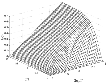
Figure 1: Entanglement of formation of the two mode amplification and damping, with the environment noise $\overline{n}_{0}=0.4$ . The initial state is vacuum state.

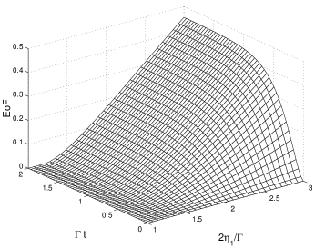
Figure 2: Entanglement of formation of the two mode amplification and damping, with the environment noise $\overline{n}_{0}=0.6$ . The initial state is vacuum state.

When $t\rightarrow\infty,$ EoF saturates at

$$E_{f}(\infty)=g(\Delta(\frac{\Gamma}{\Gamma+2\eta_{1}}[2\overline{n}_{0}+1])).$$ (54)

If the initial state is vacuum state, then $N=0,r=0.$ Inequality (52) reduces to $\alpha_{a}-\beta_{c}<\frac{1}{2}$ . It can be further simplified to

$$\eta_{1}>\max\{\overline{n}_{0}\Gamma,\frac{\Gamma}{2}\}.$$ (55)

EoFs for $\overline{n}_{0}=0.4,0.6$ are shown in Fig.1 and Fig.2. We can see that EoF is a monotonically increasing function of the amplification $\eta_{1},$ $E_{f}(\infty)$ has the same expression for $\eta_{1}>$ $\frac{\Gamma}{2}$ and $\eta_{1}<$ $\frac{\Gamma}{2}$ (see (48)). $E_{f}(\infty)$ is shown in Fig.3 (It is for any Gaussian initial state, not only for vacuum initial state). The inseparable criterion inequalities (47) and (55) can be combine

$$\eta_{1}/\Gamma>\overline{n}_{0}.$$ (56)

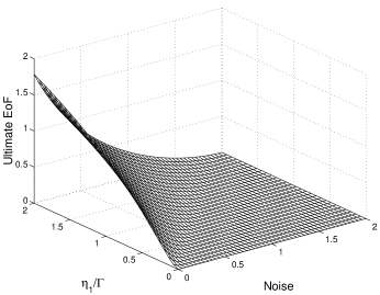
Figure 3: The ultimate entanglement of formation with respect to amplification damping ratio $\eta_{1}/\Gamma$ and environment noise $\overline{n}_{0}$

7 Conclusion

The master equation of quantum continuous variable system is converted to the equation of quantum characteristic function. It turn out to be a linear partial differential equation about the characteristic function. The time evolution solution can be obtained exactly for any initial quantum optical state in several cases. The solvable cases include (1) parametric amplification [22] , (2) amplitude damping with thermal or squeezed noise [17] , (3) simultaneously amplitude and phase damping together with thermal noise[23], (4) simultaneous multi-mode parametric amplification and amplitude damping with thermal or squeezed noise when each mode undergoes the same strength of damping, (5) simultaneous multi-mode real parametric amplification and amplitude damping with thermal or squeezed noise.

The applications to one mode and two mode Gaussian initial conditions are investigated. In one mode Gaussian system, the purity of the evolution state is monotonically decreasing with the amplification. In the situation of less amplification ($\left|\eta\right|<\Gamma/2$), the ultimate purity is maximized when the phase of the amplification $\eta$ matches with the phase of the ’squeezed’ environment $w$ . In two mode Gaussian system, the entanglement of formation monotonically increases with the two mode amplification. In the situation of less amplification ($\left|\eta_{1}\right|<\Gamma/2$), the supremum of the entanglement of formation is given. In the situation of over amplification ($\left|\eta_{1}\right|>\Gamma/2$), after a sufficient large time, the entanglement of formation saturates. The ultimate entanglement of formation is given as a function of the amplification damping ratio and the noise. It is independent of the initial Gaussian state. The ultimate state is separable when the amplification damping ratio is greater than the noise.

In real experiment, the parametric amplification and the damping may occur successively. Thus the concatenate of above solutions will represent most of the optical evolution system.

References

- [1] S. L. Braunstein and A. K. Pati Eds. Quantum Information with Continuous Variables, (Kluwer, Dordrecht, 2003).
- [2] S. L. Braunstein and P. van Loock, Rev. Mod. Phys. 77, 513 (2005).
- [3] L. Vaidman, Phys. Rev. A 49, 1473 (1994); S. L. Braunstein and H. J. Kimble, Phys. Rev. Lett. 80, 869 (1998).
- [4] A. Furusawa, J. L. Sorensen, S. L. Braunstein, C. A. Fuchs, H. J. Kimble,and E. S. Polzik, Science 282, 706 (1998); T. C. Zhang, K. W. Goh, C. W.Chou, P. Lodahl, and H. J. Kimble, Phys. Rev. A 67, 033802 (2003).
- [5] N. Takei, H. Yonezawa, T. Aoki, and A. Furusawa, Phys. Rev.Lett. 94, 220502 (2005).
- [6] P. van Loock and S. L. Braunstein, Phys. Rev. Lett. 84, 3482(2000); H. Yonezawa, T. Aoki, and A. Furusawa, Nature 431,430 (2004).
- [7] F. Grosshans and P. Grangier, Phys. Rev. Lett. 88, 057902 (2002); F.Grosshans, G. Van Assche, J. Wenger, R. Brouri, N. J. Cerf, and P. Grangier, Nature 421, 238 (2003). H. P. Yuen and A. Kim, Phys. Lett. A 241, 135 (1998); K. Bencheikh, T. Symul, A. Jankovic, and J. A. Levenson, J. Mod. Opt. 48, 1903 (2001); F. Grosshans, G. Van Assche, J. Wenger, R. Brouri, N. J. Cerf, and P. Grangier, Nature 421, 238 (2003).
- [8] P. van Loock and S. L. Braunstein, Phys. Rev. A 61, 010302(R) (2000); X. Jia, X. Su, Q. Pan, J. Gao, C. Xie, and K. Peng, Phys. Rev. Lett. 93, 250503 (2004).
- [9] M. Ban, J. Opt. B 1, L9 (1999); S. L. Braunstein and H. J. Kimble,Phys. Rev. A 61, 042302 (2000); X. Li, Q. Pan, J. Jing, J. Zhang, C. Xie, and K. Peng, Phys. Rev. Lett. 88, 047904 (2002); J. Mizuno, K. Wakui, A. Furusawa, and M. Sasaki, Phys. Rev. A 71, 012304 (2005).
- [10] B. Julsgaard, J. Sherson, J. I. Cirac, J. Fiurasek, and E. S. Polzik, Nature 432, 482 (2004).
- [11] S. Lloyd and S. L. Braunstein, Phys. Rev. Lett. 82, 1784 (1999); T. C. Ralph, A. Gilchrist, G. J. Milburn, W. J. Munro, and S. Glancy, Phys. Rev. A 68, 042319 (2003).
- [12] P. Kinsler and P. D. Drummond, Phys. Rev. A 43, 6194 (1991).
- [13] G. Lindblad, Commun. Math. Phys. 48, 119 (1976).
- [14] P. Marian, Phys. Rev. A 47, 4487 (1993).
- [15] D. Walls and G. Milburn, Quantum optics (Springer Verlag, Berlin, 1994).
- [16] A. J. Leggett, Rev. Mod. Phys. 73, 307 (2001).
- [17] A. Serafini, M.G.A. Paris, F. Illuminati, S. De Siena, J. Opt. B. 7, R19 (2005).
- [18] A. S. Holevo, M. Sohma, and O. Hirota, Phys. Rev. A 59, 1820 (1999).
- [19] P. D. Drummond, C. W. Gardiner, J. Phys. A: Math. Gen. ,13, 2353,(1980).
- [20] D. Petz, An Invitation to the Algebra of Canonical Commutation Relations, Leuven University Press, Leuven (1990).
- [21] A. Perelomov, Generalized Coherent states, Springer Verlag, Berlin (1986).
- [22] J. F. Corney, P. D. Drummond, Eprint, quant-ph/0308064, (2003).
- [23] X. Y. Chen, Phys. Rev. A, 73, 022307, (2006).
- [24] R. Simon, Phys. Rev. Lett. 84, 2726, (2000).
- [25] L. M. Duan , Giedke G, Cirac J I and Zoller P, Phys. Rev. Lett. 84, 2722 (2000).
- [26] G. Giedke, M. M. Wolf, O. Krüger, R. F. Werner, and J. I. Cirac ,Phys. Rev. Lett. 91, 107901 (2003).
- [27] X. Y. Chen, P. L. Qiu, Phys. Lett. A, 314, 191(2003).