Experimental Quantum Teleportation with a 3-Bell-state Analyzer

Abstract

We present a Bell-state analyzer for time-bin qubits allowing the detection of three out of four Bell-states with linear optics, two detectors and no auxiliary photons. The theoretical success rate of this scheme is $50\%$. A teleportation experiment was performed to demonstrate its functionality. We also present a teleportation experiment with a fidelity larger than the cloning limit of F=5/6.

I Introduction

Bell-State Analyzers (BSA) form an essential part of quantum communications protocols. Their uses range from quantum relays based on teleportation Bennett1993 ; Bouwmeester1997 ; Boschi1998 ; Waks2002 ; Jacobs2002 ; Marcikic2003 ; Collins2005 or entanglement swapping Pan1998 ; Riedmatten2005 to quantum dense coding Bennett1992 ; Mattle1996 . An important restriction for BSAs is that a system based on linear optics , without using auxiliary photons, is limited to a 50% overall success rate Calsamiglia2001 ; Knill2001 . This important result does not restrict the number of Bell-states that can be measured, but only the overall efficiency of a measurement. Nevertheless, a complete BSA is possible for at least two different cases: the first approach uses non-linear optics Kim2001 but this has the drawback of an exceedingly low efficiency and is therefore not well adapted for quantum communication protocols. Another possibility is the use of continuous variable encoding Braunstein1998 ; Furusawa1998 , however, this technique has the disadvantage that postselection is not possible. Note that postselection is a very useful technique that allows one to use only ‘good’ measurement results and straightaway eliminate all others without the need for great computational analysis.

Many experiments have been done up to date that use BSAs. In this article a novel BSA is introduced Houwelingen2006 . It has the maximum possible efficiency that can be obtained when using only linear optics without ancilla photons. It is different with respect to other BSAs since it can distinguish three out of the four Bell-states. All of the used BSAs up to date that can reach the maximum efficiency, without the use of ancilla photons, are limited to two (or less) Bell-states Weinfurther1994 ; Bouwmeester1997 ; Marcikic2003 ; Pan1998 ; Riedmatten2005 . There have also been experiments of a BSA that detects all 4 Bell-states but its overall efficiency does not reach 50% and it requires the use of an entangled ancilla photon-pair Walther2005 .

II Theory

II.1 Time-bin encoding

In our experiments a qubit is encoded on photons using time-bins Tittel1999 . This means that a photon is created that exists in a superposition of two well defined instant in time (time-bins) that have a fixed temporal separation of $\tau$. By convention the Fock-state with $N=1$ corresponding to a photon in the early time of existence $t_{0}$ is written as $|0\rangle$ and for the later time $t_{1}=t_{o}+\tau$ as $|1\rangle$. Photons in such a state can be created in several ways. The simplest method is to pass a single photon through an unbalanced interferometer with a path length difference of $nc\tau$, where $n$ is the refractive index. After the interferometer the photon will be in the qubit state $A\mbox{$|0\rangle$}+e^{i\alpha}B\mbox{$|1\rangle$}$. Here $A$ and $B$ are amplitudes that depend on the characteristics of the interferometer and $\alpha$ is the phase-difference between the interferometer paths which is directly determined by $\alpha=\frac{2\pi nc\tau}{\lambda}(\mbox{mod }2\pi)$. For sake of readability we will use the word ‘qubit’ when talking about a ‘photon that is in a qubit state’.

II.2 Bell-state Analyzer

In a large part of all experiments using Bell-state analyzers (BSAs) that have been performed up to date, the BSA consists essentially of a beamsplitter and single photon detectors (SPDs). In such a beamsplitter-BSA(BS-BSA) the ‘clicks’ of the SPDs are analyzed and, depending on their results, the input state will be projected onto a particular Bell-state. With time-bin qubits as described above a simple BS-BSA works as follows: two qubits arrive at the same time on a beamsplitter but at different entry ports. Since the 4 standard Bell-states

$$\mbox{$|\phi_{\pm}\rangle$}=\frac{1}{\sqrt{2}}(\mbox{$|00\rangle$}\pm\mbox{$|11\rangle$})$$ (1)

$$\mbox{$|\psi_{\pm}\rangle$}=\frac{1}{\sqrt{2}}(\mbox{$|01\rangle$}\pm\mbox{$|10\rangle$})$$ (2)

form a complete basis we can write our 2-qubit input-state as a superposition of these four states. One can calculate for each Bell input-state the possible output states. These states can then be detected using SPDs. The different detection patterns and their probabilities are shown in Table 1.

D1	00		11		01		0	0	1	1
D2		00		11		01	0	1	0	1
$|\phi_{+}\rangle$	1/4	1/4	1/4	1/4
$|\phi_{-}\rangle$	1/4	1/4	1/4	1/4
$|\psi_{+}\rangle$					1/2	1/2
$|\psi_{-}\rangle$								1/2	1/2

Table 1: The table shows the probability to find specific coincidences as a function of the input Bell-state in the case of a single beamsplitter as a BSA. A ‘0’(‘1’) in row D1 means that a photon was found at detector ‘D1’ at time $t_{0}$($t_{1}$) etc. Note that only half of the combinations of detection are possible for only one Bell-state(the bold entries), therefore when such a combination is found a projection onto this Bell-state was performed. The theoretical success-probability is 50%.

By convention, a detection click at time ‘0’(‘1’) means that the photon was detected in time-bin $t_{0}$($t_{1}$). The output combinations show that, if one detects two photons in the same path but in a different time-bin, the input state could only have been caused by the Bell-state $|\psi_{+}\rangle$ and therefore the overall state of the system is projected onto this state. When the photons arrive at different detectors with a time-bin difference the input-state is projected onto the state $|\psi_{-}\rangle$. However, when one measures two photons in the same time-bin in the same detector the state could either be $|\phi_{+}\rangle$ or $|\phi_{-}\rangle$ and therefore the state has not been projected onto a single Bell-state but onto a superposition of two Bell-states. This method has a success rate of 50% which corresponds to the maximal possible success rate that can be obtained while using only linear optics and no auxiliary photons Calsamiglia2001 .

Here we propose a new BSA which is capable of distinguishing more than 2 Bell-states while still having the maximum success rate of 50%. This is possible by replacing the beamsplitter with a time-bin interferometer equivalent to the ones used to encode and decode time-bin qubits (Fig. 1). This BSA will be capable of distinguishing three out of four Bell-states, but $|\phi_{+}\rangle$ and $|\psi_{-}\rangle$ will only de discriminated 50% of the time as will be explained shortly.

Figure 1: A schematic representation of the new type of Bell-state Measurement. When two qubit states are sent into a time-bin interferometer the output state is a mixture of photons in two directional modes and three temporal modes. By looking at certain combinations of these photons a Bell-state measurement can be performed for three different Bell-states

Two qubits enter in port $a$ and $b$, respectively. The first beamsplitter acts like above, allowing the distinction of two Bell-states ($|\psi_{+}\rangle$ and $|\psi_{-}\rangle$). A second possibility for interference is added by another BS for which the inputs are the outputs of the first BS, with one path having a delay corresponding to the time-bin separation $\tau$. The two-photon effects on this beamsplitter leads to fully distinguishable photon combinations of one of the two remaining Bell states ($|\phi_{+}\rangle$) while still allowing a partial distinction of the first two.

One might expect that when it is possible to measure three out of four states that the fourth, non-measured, state can simply be inferred from a negative measurement result of the three measurable states. This is, however, not the case. The above described measurement is a POVM with $21$ possible outcomes, some of these outcomes are only possible for one of the four input Bell-states. Therefore when such an outcome is detected it unambiguously discriminates the corresponding input Bell-state. The rest of the $21$ outcomes correspond to outcomes which can result from more than one input Bell-state. In other words, their results are ambiguous and the input state is not projected onto a single Bell-state but onto a superposition of Bell-states.

The state after the interferometer can be calculated for any input-state using:

$$\hat{a}^{\dagger}(t)\Rightarrow\frac{1}{\sqrt{4}}( -\hat{e}^{\dagger}(t)+e^{i\delta}\hat{e}^{\dagger}(t+\tau)$$ (3)

$$+i\hat{f}^{\dagger}(t)+ie^{i\delta}\hat{f}^{\dagger}(t+\tau) )$$

$$\hat{b}^{\dagger}(t)\Rightarrow\frac{1}{\sqrt{4}}( \hat{f}^{\dagger}(t)-e^{i\delta}\hat{f}^{\dagger}(t+\tau)$$ (4)

$$+i\hat{e}^{\dagger}(t)+ie^{i\delta}\hat{e}^{\dagger}(t+\tau) )$$

where $\hat{i}^{\dagger}(j)$ is the creation operator of a photon at time $j$ in mode $i$. When the input-states are qubits and the photons are detected after the interferometers the detection-patterns are readily calculated and are shown in Table 2.

$D1$	00		11		22		01		02		12		0	2	1	1	0	1	2	0	2
$D2$		00		11		22		01		02		12	0	2	1	0	1	2	1	2	0
$|\phi_{+}^{\prime}\rangle$	1/16	1/16			1/16	1/16							1/8	1/8	1/2
$|\phi_{-}^{\prime}\rangle$	1/16	1/16	1/4	1/4	1/16	1/16							1/8	1/8
$|\psi_{+}^{\prime}\rangle$							1/8	1/8			1/8	1/8				1/8	1/8	1/8	1/8
$|\psi_{-}^{\prime}\rangle$			1/4	1/4					1/8	1/8										1/8	1/8

Table 2: The table shows the probability to find any of the 21 possible coincidences as a function of the input Bell-state. A ‘0’ in row D1 means that a photon was found at detector ‘D1’ and at a time corresponding to the photon having taken the short path in the interferometer and it was originally a photon in time-bin $t_{0}$, a ‘1’ corresponds to $t_{0}+\textbf{1}\times\tau$ with $\tau$ corresponding to a the difference between the time-bins etc. Note that several combinations of detection are possible for only one Bell-state(the bold entries), therefore when such a combination is found a Bell-state Measurement was performed. The theoretical probability of a successful measurement is 0.5 which is the optimal value using only linear optics Calsamiglia2001 .

The output coincidences on detectors $D1\mbox{ (port $e$)}$ and $D2\mbox{ (port $f$)}$ are shown as a function of a Bell-state as input. By convention, a detection at time ‘0’ means that the photon was in time $t_{0}$ after the BSA-interferometer. This is only possible if it took the short path in the BSA and it was originally a photon in time-bin $t_{0}$ (Fig. 1). Similarly a detection at time ‘1’ means that either the photon was originally in $t_{1}$ and took the short path of the BSA interferometer or it was in $t_{0}$ and took the long path. A detection at time ‘2’ means the photon was in $t_{1}$ and took the long path. In Table 2 we see that some of the patterns corresponds to a single Bell-state and therefore the measurement is unambiguous. For the other cases the result could have been caused by two Bell-states, i.e. the result is ambiguous and hence inconclusive. More specifically, the Bell-state $|\psi_{+}^{\prime}\rangle$ is detected with probability 1, $|\phi_{-}^{\prime}\rangle$ is never detected and both $|\psi_{-}^{\prime}\rangle$ and $|\phi_{+}^{\prime}\rangle$ are detected with probability 1/2.

The above described approach is correct in the case were the separation $\tau$ of the incoming qubits is equal to the time-bin separation caused by the interferometer. If this in not the case and the interferometer creates a time-bin seperation of $\tau+\frac{n\lambda\delta}{2\pi c}$, where $\delta$ is a phase, the situation is slightly more complicated In such a case, our BSA still distinguishes 3 Bell-states, but these are no longer the standard Bell-states but are the following:

$$|\phi^{\prime}_{\pm}\rangle = \mbox{$|00\rangle$}\pm e^{2i\delta}\mbox{$|11\rangle$}=(\sigma_{\delta}\otimes\sigma_{\delta})\mbox{$|\phi_{\pm}\rangle$}$$ (5)

$$|\psi^{\prime}_{\pm}\rangle = e^{i\delta}(\mbox{$|01\rangle$}\pm\mbox{$|10\rangle$})=e^{i\delta}\mbox{$|\psi_{\pm}\rangle$}$$ (6)

Here $\sigma_{\delta}=P_{\mbox{$|0\rangle$}}+e^{i\delta}P_{\mbox{$|1\rangle$}}$ is a phase shift of $\delta$ to be applied to the time bin $|1\rangle$. These new Bell-states are equivalent to the standard states except that the $|1\rangle$ is replaced by $e^{i\delta}\mbox{$|1\rangle$}$ for each of the input modes.

In a realistic experimental environment the success probabilities of the BSA are affected by detector limitations. This is because existing photon detectors are not fast enough to distinguish photons which follow each other closely (in our case two photons separated by $\tau=1.2$ ns) in a single measurement cycle. This limitation rises from the dead time of the photodetectors. When including this limitation we find that the maximal probabilities of success in our experimental setup are reduced to $1/2$, $1/4$ and $1/2$ for $\psi_{+}$, $\psi_{-}$ and $\phi_{+}$, respectively. This leads to an overall probability of success of $5/16$ which is greater by $25\%$ than the success rate of $1/4$ for a BSA consisting only of one beamsplitter and two detectors with the same limitation. This limitation could be partially eliminated by using a beamsplitter and two detectors in order to detect the state 50% of the time, or it could be completely eliminated by using an ultra-fast optical switch (sending each time-bin to a different detector). Both of these methods are associated with a decrease in signal-to-noise ratio. This is caused by additional noise from the added detector and by additional losses from the optical switch, respectively.

II.3 Bell-state analyzer for polarization qubits

So far the discussion about this BSA only considered time-bin qubits. The authors would like to note at this point that it is also possible to implement a similar BSA for polarization encoded photons. This can be done by the equivalent polarization setup as shown in Fig. 2. This setup would require 4 detectors but there will never be two photons on one detector and therefore dead-times don’t hinder the measurement of all the detection patterns and the overall efficiency can reach 50% with today‘s technology.

Figure 2: A schematic representation of the new type of Bell-state Analyzer for polarization qubits. The grey cubes represent non-polarizing beamsplitters and the white cubes are polarizing beamsplitters.

II.4 4-Bell-state analyzer?

This paper discusses our results testing a 3-Bell-state analyzer. It is obviously interesting to also consider the possibility of a linear optics 4-Bell-state analyzer with 50% efficiency and no ancilla photons. Such a system was not used for the simple reason that there is no known method to make such a measurement. Is there a fundamental reason to suspect that such a BSA cannot be performed? No such reason is known to the authors, therefor this article will be limited to the 3-Bell-state analyzer.

II.5 Teleportation

One of the most stunning applications of a BSA is its use in the teleportation protocol. In order to perform a teleportation experiment an entangled qubit photon pair is created (EPR Einstein1935a ) as well as a qubit to be teleported(Alice). One photon of the entangled pair is made to interact with Alices qubit in a BSA (Charly). This interaction followed by detection projects the overall state onto a Bell-state (if the BSA is successful). The remaining photon (Bob) now carries the same information as the photon from Alice up to a unitary transformation. The situation for the new BSA is slightly different since the entangled pair is not a member of the detected Bell-basis (Eq. 5 and 6). However this has no major influence on the theory. After a succesful measurement of the BSA the remaining photon at Bob is equal to the original qubit up to a unitary transformation. This transformation however has to be adapted with regards to the standard case from [$\openone$,$\sigma_{z}$,$\sigma_{x}$,$\sigma_{x}\sigma_{z}$] to [$\sigma_{2\delta}^{-1}$,$\sigma_{z}\sigma_{2\delta}^{-1}$,$\sigma_{x}$,$\sigma_{x}\sigma_{z}$], as can be seen from the following calculation.

$$\mbox{$|\zeta_{abc}\rangle$}=\mbox{$|\zeta\rangle$}_{a} \otimes |\phi_{+}\rangle$$ (7)

$$=\frac{1}{2}(\mbox{$|\phi^{\prime}_{+}\rangle$}_{ab} \otimes \sigma_{2\delta}^{-1}\mbox{$|\zeta\rangle$}_{c}$$ (8)

$$+\mbox{$|\phi^{\prime}_{-}\rangle$}_{ab} \otimes \sigma_{z}\sigma_{2\delta}^{-1}\mbox{$|\zeta\rangle$}_{c}$$

$$+\mbox{$|\psi^{\prime}_{+}\rangle$}_{ab} \otimes e^{-i\delta}\sigma_{x}\mbox{$|\zeta\rangle$}_{c}$$

$$+\mbox{$|\psi^{\prime}_{-}\rangle$}_{ab} \otimes e^{-i\delta}\sigma_{x}\sigma_{z}\mbox{$|\zeta\rangle$}_{c}$$

Recall $\sigma_{2\delta}^{-1}=P_{\mbox{$|0\rangle$}}+e^{-2i\delta}P_{\mbox{$|1\rangle$}}$ is a phase shift of the bit $|1\rangle$.

III Experimental Teleportation

The new BSA was tested in a quantum teleportation experiment. Presented in this section are the experimental setup that was used as well as some of the required preliminary alignment experiments. Finally the results of the experiment are given and discussed.

III.1 Experimental setup

A rough schematic of the experimental setup is shown in Fig. 3, the experiment is an adaptation of a setup used previously for long distance teleportation Marcikic2003 and for entanglement swapping Riedmatten2005 .

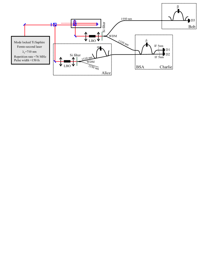
Figure 3: A rough overview of the experimental setup. The fiber interferometers shown here are in reality Michelson-interferometers, for the interferometer in the BSA two circulators are used to have two separate inputs and outputs. Not shown in the figure is the method used for stabilizing the interferometers.

Alice prepares a photon in the state $\mbox{$|\zeta\rangle$}_{a}=\frac{1}{\sqrt{2}}(\mbox{$|0\rangle$}+e^{i\alpha}\mbox{$|1\rangle$})$. A BSA is used by Charly on Alices qubit combined with a part of an entangled qubit pair. Bob analyzes the other half of the pair (the teleported qubit) and measures interference fringes for each successful BSA announced by Charly.

The setup consist of a mode-locked Ti-sapphire laser (MIRA with 8W VERDI pump-laser, Coherent) creating 150fs pulses with a spectral width of 4nm, a central wavelength of 711nm, a mean power of 400mW and a repetition-rate of 80MHz. This beam is split in two beams using a variable coupler ($\lambda/2$ and a PBS). The reflected light (Alice) is sent to a scannable delay and afterwards to a Lithium tri-Borate crystal(LBO, Crystal Laser) where by parametric down-conversion a pair of photons is created at 1.31 and 1.55 $\mu$m. Pump light is suppressed with a Si-filter, and the created photons are collected by a single mode optical fiber and separated with a wavelength-division-multiplexer (WDM). The 1.55 $\mu$m photon is ignored, whereas the photon at 1.31 $\mu$m is send to a fiber interferometer which encodes the qubit state $\mbox{$|\zeta\rangle$}_{a}$ onto the photon. The transmitted beam (Bob) is passed through an unbalanced Michelson-type bulk interferometer. The seperation between the two time-bins after this interferometer is considered as the reference for all the other seperations. The phase of the interferometer can therefore be considered as a reference phase and can be defined as 0. After the interferometer the beam passes a different LBO crystal. The non-degenerate photons-pairs created in this crystal are entangled and their state corresponds to $\mbox{$|\phi_{+}\rangle$}=\frac{1}{\sqrt{2}}(\mbox{$|00\rangle$}+\mbox{$|11\rangle$})$.

The photons at 1.31$\mu$m are send to Charly in order to perform the Bell-state measurement. To assure temporal indistinguishability, Charly filters the received photons down to a spectral width of 5nm using a bulk interference filter. Because of this the coherence time of the generated photons is greater than that of the photons in the pump beam, and as such no distinguishablity between photons can be caused by jitter in their creation time Riedmatten2003 . Bob filters his 1.55$\mu$m photon to 15nm in order to avoid multi photon-pair events Riedmatten2004 ; Scarani2005a , this filtering is done by the WDM that separates the photons at 1.31 and 1.5$\mu$m. This filter is larger than Charlies filter for experimental reasons. A liquid Nitrogen cooled Ge Avalanche-Photon-Detector (APD) D1 with passive quenching detects one of the two photons in the BSA and triggers the InGaAs APDs (id Quantique) D2 and D3. Events are analyzed with a time to digital converter (TDC, Acam) and coincidences are recorded on a computer.

Each interferometer is stabilized in temperature and for greater stability an active feedback system adjusts the phase every $100$ seconds using reference lasers. The reference for Bob‘s interferometer is a laser (Dicos) stabilized on an atomic transition at 1531nm and for both Alice‘s and Charlies interferometer a stabilized DFB-laser (Dicos) at 1552nm is used. It is possible to use different lasers for Alice and Charly if one wants to create two independent units. By using independent interferometer units using different stabilization lasers it was assured that this experiment is ready for use ‘in the field’. A more detailed description of the active stabilization of the interferometers is given in ref Riedmatten2005 . For sake of clarity the interferometers shown in the setup (Fig. 3) are Mach-Zender type interferometers but in reality they are Michelson interferometers which use Faraday-mirrors in order to avoid distinguishability due to polarization differences Tittel2001 .

III.2 Alignment experiments

There are two important, non-trivial alignments that have to be made before one can perform a quantum teleportation experiment with time-bin encoded qubits. First, one would have to assure that all the time-bin interferometers have the same difference in length between the two paths. Second, it is required that there is temporal indistinguishability between qubits coming from Alice and Bob on the BSA. The equalization of the interferometers is needed in order to assure that all the interferometers have a difference in length of $\frac{c\tau}{n}$ with a precision higher than the coherence length of the photons ($\approx$150$\mu m$). We have two mechanisms to actively change the optical path lengths: the first is changing the temperature of the interferometers and thus allowing the long arm to increase/decrease its length more than the short arm, the second is to directly change the length of only one arm by means of a cylindric piezo-electric element. When changing the voltage over the piezo we change the diameter of the cylinder and thus the length of the fiber changes. This is used for the active feedback stabilization system. In order to align the interferometers with each other we perform two different experiments: First, we optimize the visibilty of single photon interference fringes for photons from Alice detected in $D1$. This aligns Alices interferometer with the BSA interferometer. Next, we optimize a Fransson-type Bell-test of the entangled photon-pair Franson1989 . While optimizing this experiment we do not change the BSA-interferometer. This optimization aligns the bulk-interferometer and Bobs analysis interferometer to the other two. Using this method we found visibilities of $97\%\pm 1\%$ for the single photon interference and $94\%\pm 1\%$ for the Bell-test (Fig. 4).

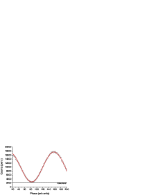
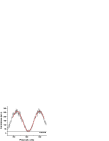
Figure 4: Left: Single photon interference with $V_{net}=0.97\pm 0.01$. Right: Fransson-type Bell-test with $V_{net}=0.94\pm 0.01$.

The second alignment procedure is necessary in order to assure temporal indistinguishability between the photons arriving at the BSA. In the case of a BS-BSA this can be assured by performing a Hong-Ou-Mandel dip type experiment Hong1987 , which is to say, make a scan in a delay for one of the incoming photons and look at a decrease in the number of coincidences as a result of photon bunching (Fig. 5). The position where the minimum is obtained corresponds to the point with maximal temporal overlap of the two photons.

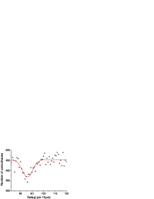
Figure 5: Left, IF-BSA: Graph showing the number of measured coincidences as a function of a change in the delayline. Both ‘00’ and ‘22’ clearly show an antidip at the same location. The net visibilties are $V_{00}=32\pm 3\%$ and $V_{22}=26\pm 2\%$ Right, BS-BSA: Graph showing the decrease in the number of measured coincidences ‘00’ as a function of a change in the delayline Hong1987 . The net visibility is $V=29\pm 3\%$.

In the case of an interferometer-BSA (IF-BSA) this procedure becomes more complicated. We can no longer look at a mandel dip because the second beamsplitter will probabilistically split up the photons that bunched on the first beamsplitter. However the photon bunching remains and it can still be seen by a different method. Consider the situation where two single photons, both in the state $|0\rangle$, are send to the different inputs of an IF-BSA (Fig. 6). If the photons are not temporally indistinguishable there are three possible output differences between detection times, corresponding to ‘10’, ‘00&11’ and ‘01’. If the photons are indistinguishable they bunch at the first BS and therefore the difference in arrival time between the photons has to be zero. This means that ‘10’ and ‘01’ are not possible anymore and the possibility for ‘00&11’ is larger.

Figure 6: The simple experiment on the left (one photon in each input of an IF-BSA) will have the following property. If the photons are not temporally indistinguishable one will find three different coincidence peaks: ‘10’,‘00&11’ and ‘01’ (dotted curve), however, if the photons are indistinguishable there will be only one peak: ‘00&11’(plain curve). This is caused by photon bunching.

If the inputs are arbitrary qubits instead of the simple example above there will be more coincidence possibilities and some of them will be subject to single-photon interference and/or photon bunching. It is possible to see an increase in the coincidences for ‘00’ and ‘22’, which is not affected by single-photon interference, for similar reasons as the increase that was explained above. These coincidences can be measured in a straightforward way with our setup. A more rigorous calculation and explication of this alignment procedure is given in the appendix. A typical result of an experiment in which the count rate is measured while changing a delay is shown in Fig. 5 and clearly shows the expected increase in count rate.

The measured antidips have a net visibility of $32\pm 3\%$ and $26\pm 2\%$ after noise substraction. The maximal attainable value is $1/3$ due to undesired but unavoidable double-pair events (see appendix). The large visibilities mean that the temporal indistinguishability is very good, this will thus not be limiting for our experiments. The noise substraction for this estimation is justified because in a teleportation experiment the noise will be reduced since one will consider only 3-photon events. The difference in height of the two coincidences is related to an electronic loss of signal in an electrical delay line.

III.3 Experimental Results

Two different types of teleportation experiments were performed. Namely a standard BS-BSA teleportation in order to benchmark our equipment followed by the new IF-BSA experiment. For the BS-BSA the main difference with regards to previous experiments Riedmatten2004 ; Riedmatten2005 was that the interferometers now all had an active stabilization. This allows for large stability and long measurement times. The experiment consisted of Bob scanning of his interferometer phase while the other interferometers where kept constant, we therefore expect to find an interference curve of the form $1+Vsin(\beta+\alpha)$ where $\alpha$ is kept constant. The results of the experiment (Fig. 7) clearly shows the expected behavior.

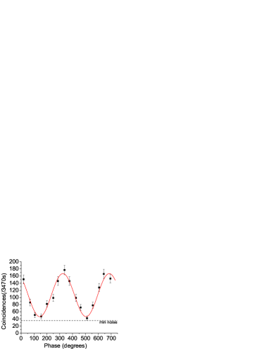
Figure 7: The Result of the 1-Bell state teleportation experiment (a beamsplitter instead of the interferometer) with $F_{raw}=0.79\pm 0.02$ and $F_{net}=0.91\pm 0.02$.

The visibility measured was $V=0.57\pm 0.03$ ($F=0.79\pm 0.02$). After conservative noise substraction we find $V=0.83\pm 0.04$ ($F=0.91\pm 0.02$). This clearly is higher than the strictest threshold that has been associated with quantum teleportation of $F=5/6$ Grosshans2001 ; Bruss1998a . The limiting factors of this experiment are the detectors and the fiber-coupling after the LBO crystals.

After this experiment the setup was changed to the IF-BSA. The count-rates in this experiment with regards to the previous one is reduced due to two reasons. The introduction of the BSA-interferometer and its stabilization optics means an additional 3dB of loss which reduces count rates. Another difference is that now the counts are distributed over three different Bell-states whereas before there was only one. Therefore an overall reduction of counts per state will occur. Combined these effects result in a large reduction of the count rate per Bell-state. This problem was overcome by, on one hand, an overall increase of the BSA efficiency by 1/4 (from 25% for the BS-BSA to 31.25% for the IF-BSA) and, on the other hand, by integrating data over longer time periods. During the teleportation-experiment scans were made in the interferometer of Alice rather than Bob. This was done since the most important noise is dependant of the phase of Bob‘s interferometer but not of Alice‘s (more details are given in the next subsection). The experiments were performed with approximately 4.4 hours per phase setting in order to have low statistical noise.

For this IF-BSA all the different unambiguous results (Table 2) where analyzed both separately (for example ‘02’) and combined as a Bell-state (for example $\mbox{$|\psi_{-}\rangle$}=$‘02’$+$‘20’). For the separate results it is expected that each BSA outcome will have count rates depending on the phases of the interferometers as $R(1+Vcos(\alpha+\rho))$. Here $R$ is dependant of the overall efficiency of the experiment and is different for each BSA outcome and $\rho$ is a combination of the constant phases of the interferometers of Bob and Charlie and is different for different BSA results:

$$\mbox{$|\psi_{+}\rangle$},\mbox{$|01\rangle$},\mbox{$|10\rangle$},\mbox{$|12\rangle$},\mbox{$|21\rangle$} \rightarrow \rho=\beta$$ (9)

$$\mbox{$|\phi_{+}\rangle$},\mbox{$|11\rangle$} \rightarrow \rho=-\beta-2\delta$$ (10)

$$\mbox{$|\psi_{-}\rangle$},\mbox{$|02\rangle$},\mbox{$|20\rangle$} \rightarrow \rho=\beta+\pi$$ (11)

As is evident from the differences in $\rho$ we expect that fringes corresponding to one particular Bell-state are in phase with each other, but have a well determined phase-difference with fringes corresponding to another Bell-state.

The measured count rates as a function of the phase of Alices interferometer are shown in (Fig. 8).

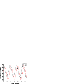
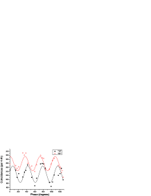
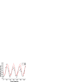
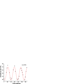
Figure 8: Measured coindance counts as a function of phase. Top-Left: BSA-results ‘01’, ‘10’. Top-Right: BSA-results ‘12’, ‘21’. Bottom-Left: BSA-results ‘02’ and ‘20’. Bottom-Right: BSA-results ‘11’. Note that for each graph there is an unknown, but equal, offset of the phase-value.

Note that, due to experimental restrictions, the absolute phases of the interferometers are not known and therefor all phase-values have an unknown offset. The results clearly show that each of the outcomes has the expected interference behavior. Furthermore, the fringe corresponding to ‘01’ is in phase with the fringe ‘21’. The same is true for the fringe ‘10’ with ‘12’ and for ‘02’ with ‘20’. It is expected that all four of the fringes corresponding to $|\psi_{+}\rangle$ (‘01’,‘10’,‘12’ and ‘21’) are all in phase with each other, but there is a clear phase-shift between the first two and the last two. The average phase of these four fringes is different by $180^{o}$ from the fringes corresponding to ‘02’ and ‘20’ as expected. The fringe corresponding to ‘11’ is in phase with the fringes of ‘02’ and ‘20’ as was expected since for this measurement we had arranged $2(\beta+\delta)=\pi(\mbox{mod}2\pi)$. The results of the fits to these fringes is shown in Table 3. The differences in phase and visibility are in part due to noise (see next subsection)

Result 3BSA		$V_{raw}$	$V_{net}$	$\rho_{raw}$	$\rho_{net}$	$P_{raw}$	$P_{net}$
$|\psi_{+}\rangle$	$|01\rangle$	35$\pm$ 3	61$\pm$ 6	278 $\pm$ 4	279$\pm$5	13$\pm$1	14$\pm$1
	$|10\rangle$	43$\pm$ 3	72$\pm$ 13	339 $\pm$ 4	338$\pm$8	11$\pm$1	13$\pm$1
	$|12\rangle$	18$\pm$ 3	64$\pm$ 7	340 $\pm$ 7	340$\pm$4	14$\pm$1	7$\pm$1
	$|21\rangle$	13$\pm$ 2	36$\pm$ 2	227 $\pm$ 9	278$\pm$1	17$\pm$1	10$\pm$1
$|\phi_{+}\rangle$	$|11\rangle$	43$\pm$ 3	55$\pm$ 2	136 $\pm$ 3	136$\pm$10	29$\pm$1	41$\pm$1
$|\psi_{-}\rangle$	$|02\rangle$	40$\pm$ 5	83$\pm$ 13	126 $\pm$ 12	126$\pm$8	8$\pm$1	6$\pm$1
	$|20\rangle$	39$\pm$ 4	62$\pm$ 10	153 $\pm$ 4	153$\pm$8	9$\pm$1	9$\pm$1
$|\psi_{+}\rangle$		$22\pm 1$	$51\pm 3$	311 $\pm$ 3	311$\pm$ 3	54$\pm$1	43$\pm$1
$|\phi_{+}\rangle$		$43\pm 3$	$55\pm 2$	136 $\pm$ 10	136$\pm$ 3	29$\pm$1	41$\pm$1
$|\psi_{-}\rangle$		$38\pm 5$	$69\pm 10$	140 $\pm$ 6	140$\pm$ 7	17$\pm$1	15$\pm$1

Table 3: For each of the different detection possibilities the fitted result are shown before and after noise correction.‘$V$’ refers to the Visibility (%), ‘$\rho$’ to the phase of the fringes (degrees, unknown offset) and ‘P’ to the normalized probabilities of a coincidence detection (%) . The last three rows correspond to fits made after adding the corresponding BSA outcomes, therefore these values can be slightly different from the average of the individual results.

The results corresponding to each of the three possible Bell-states can be found by adding the measurements of the constituent parts. When doing this one would expect coincidence fringes of the form $R(1+Vcos(\alpha+\rho))$ with $R$ and $\rho$ as above. This corresponds to three distinct interference fringes, with $|\phi_{+}\rangle$ and $|\psi_{-}\rangle$ in phase and $|\psi_{+}\rangle$ with a $180^{o}$ phase-difference with respect to the other two.

In Fig. 9 we show the raw coincidence interference fringes between detection rate at Bob and a successful BSA as a function of a change of phases in Alices interferometer. As expected fringes for $|\psi_{-}\rangle$ and $|\psi_{+}\rangle$ have a $180^{o}$ phase difference due to the phase flip caused by the teleportation. On the other hand the fringe for $|\phi_{+}\rangle$ is in phase with the $|\psi_{+}\rangle$ as expected. The raw visibilities obtained for the projection on each Bell-state are $V_{\psi_{-}}=0.38\pm 0.05$, $V_{\psi_{+}}=0.22\pm 0.01$, $V_{\phi_{+}}=0.43\pm 0.03$ which leads to an overall value of $V=0.34\pm 0.06$ ($F=0.67\pm 3$). In order to check the dependence of $|\phi_{+}\rangle$ on $\delta$ we also performed a teleportation with a different value for $\delta$ and we clearly observe the expected shift in the fringe (Fig. 10) while measuring similar visibilities.

Note that Bob is able to derive the phase value $\delta$ of the BSA interferometer just by looking at the phase differences between the fringes made by $\psi_{\pm}$ and $\phi_{+}$ and his knowledge about $\beta$. It is important to know $\delta$ since this allows Bob to perform the unitary transformation $\sigma_{2\delta}$ on the teleported photon.

Since the count rates were quite low we expected to have an important noisefactor, an analysis of the noise follows in the next subsection.

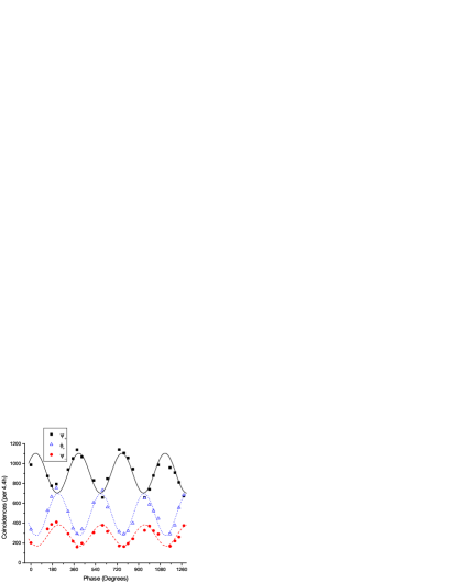
Figure 9: Uncorrected teleportation fringes found when scanning the interferometer at Bob. The fitted curves have visibilities of 0.22,0.43 and 0.38 for $|\psi_{+}\rangle$, $|\phi_{+}\rangle$ and $|\psi_{-}\rangle$. The average visibility of the BSA is $V_{avg}=0.34$ (F=0.67).

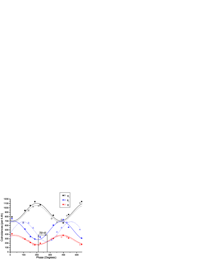
Figure 10: Teleportation fringes measured in two distinct measurement with a $\delta$ which had changed by $70\pm 10^{o}$. In the measurement a clear shift is visible of the fringe $|\phi_{+}\rangle$ by $74^{o}$ with regards to the other fringes.

III.4 Noise Analysis and Discussion

In the case of the BS-BSA the noise analysis is straightforward. All of the important noise counts are completely independent of the phase, since they concern situations in which there is no single-photon interference possible. The most important sources of noise were estimated and then measured. The estimated SNR was $2.6$, measurements find a SNR of approximately $2.2\pm 0.5$. The largest source of noise are darkcounts at one detector combined with two real detections.

The situation for the IF-BSA is more complicated. The additional interferometer has an unfortunate side-effect. There are now possibilities for noise to depend on the phases of the interferometers. In other words, while measuring interference fringes there are also noise fringes. It it obviously important to be able to distinguish between the two. The most important fluctuating noise is caused by false coincidence-detections that involve one (or more) photons coming from Alice and no photons from the EPR-source at the BSA. These noise sources depend on the phases $\alpha$ and $\delta$ since the photon coming from Alice experiences single-photon interference. Since during the experiment $\alpha$ is changed the noise-rate also changes. The period of this change is the same as for teleportation, however, there is a $\pi$ phaseshift between ‘01’(‘21’) and ‘10’(‘12’) that is not present in the teleportation signal. Such a noise influences the results of our measurements in different ways, first of all, the visibilities are altered and are smaller for ‘01’ and ‘21’ but larger for ‘10’ and ‘12’. Secondly, when the fringe is not in phase with the teleportation signal there is a phaseshift in the opposite direction for ‘01’ and ‘21’ with regards to ‘10’ and ‘12’. In our measurements the phases were arranged in such a way that this second effect would not take place since the fringes would be completely in or out of phase with the teleportation signal. This noise was measured and the result (Fig. 11) clearly shows the expected fringes and phaseshifts.

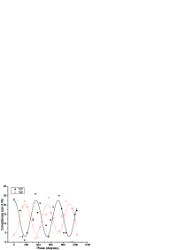
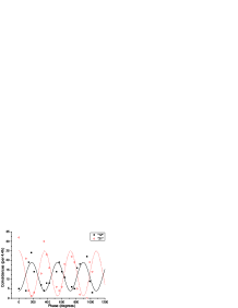
Figure 11: Measurements of the Noise for a interferometer-BSA teleportation experiment. Left: ‘01’ and ‘10’ are in antiphase as expected and have Visibilities of $V_{01}=0.77\pm 0.12$, $V_{10}=0.65\pm 0.12$ Right: ‘12’ and ‘21’ have a $\pi$ phaseshift as expected and have Visibilities of $V_{12}=0.66\pm 0.14$, $V_{21}=0.91\pm 0.13$

Other possibilities for fluctuating noise sources are when no photons from Alice arrive at the BSA. In this case single (or multiple) photon-pairs from the EPR-source combined with darkcounts will give coincidences that depend on the phases $\beta$ and $\delta$. This corresponds to a combination of a Fransson-type Bell-test with a darkcount. The fluctuation of this noise was avoided in our experiment since we only changed the phase of Alices interferometer($\alpha$).

Not all possible sources of noise depend on the phases of the interferometers, there are also stable sources of noise, which are different for each of the BSA-possibilities. The average value of the most important noise sources are shown in table 4, which shows that by choosing to scan Alice instead of Bob a large fluctuating noise was avoided.

		01			02			10			11			12			20			21
Source Alice Blocked	70	$\pm$	4	60	$\pm$	4	60	$\pm$	4	88	$\pm$	6	147	$\pm$	6	46	$\pm$	3	157	$\pm$	5
EPR to Bob Blocked	2.7	$\pm$	0.1	1.0	$\pm$	0.1	3.5	$\pm$	0.1	5.3	$\pm$	0.1	4.3	$\pm$	0.1	1.7	$\pm$	0.1	4.2	$\pm$	0.1
EPR to BSM Blocked	13	$\pm$	1	7	$\pm$	1	12	$\pm$	1	15	$\pm$	1	11	$\pm$	1	7.8	$\pm$	1	13.07	$\pm$	1

Table 4: The average noisecounts of several noise possibilities. Note that each measured value concerns a combination of different sources of noise. The most important noise (source Alice blocked) didn’t fluctuate during the experiment because the scan in phase was done by Alice.

It also shows the fluctuating noise from Alice is only a small part of the total noise and therefore its effect will only be limited. Another source of errors that is different for each coincidence combination is electronical loss. These losses are caused by long (up to 100 ns) electronical delays that are required in the treatment of the coincidence signals.

The results, after noise-substraction and correction for electronical transmission differences for the individual coincidence combinations, are shown in table 3. There is a clear agreement with theory, for example the probability of finding a ‘11’ is approximately $4$ times larger than the probability for any of the other possibilities (Fig. 12).

There are a few noteworthy differences between the results and theory. First of all there are small differences in visibility, these are probably caused by several small unmeasured noise sources and partially they are real physical differences which are caused by imperfect interferometers, an indication of these imperfections is given by the quality of the alignment experiments. Second the phases of the curves show an interesting phase difference between ‘01’(‘12’) and ‘10’(‘21’). The reason for this shift is unknown, but the average value of the two phases corresponds with the phase that is expected from the curve for ‘02’ and ‘20’. This suggests that this effect is caused by a fluctuating noise that is out of phase with the teleportation fringe.

Figure 12: Normalized probabilities of detecting a coincidence or a Bell-state. The expected value for the coincidence ‘11’ is $0.4$ and for the other coincidances $0.1$. For the Bell-state $|\psi_{-}\rangle$ one expects $0.2$ and $0.4$ for $|\psi_{+}\rangle$ and $|\phi_{+}\rangle$.

When the different possibilities of the BSA are summed, in order to have the Bell-states, the noise will no longer have any fluctuations. This is because the different noise-possibilities had a $\pi$ phase difference. After summing the different parts of the noise of a Bell-state the result will be constant. For example, the noise of ‘01’ combined with ‘10’ is approximately constant. The overall resulting noise is in practise independent of the phase. The results after noise substraction and correction for electronic transmission differences are shown in Fig 13 and Table 3 .

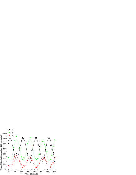
Figure 13: Result of the Teleportation experiment using an interferometer Bell-state analyzer. These results are corrected for noise and electronic differences.

The results show excellent correspondence between theory and experiment. The visibilities are similar within their errors. The difference in phase between $|\psi_{+}\rangle$ and $|\psi_{-}\rangle$ ($189^{o}\pm 9^{o}$) corresponds with theory ($180^{o}$). Also, since the phases were arranged in such a way that $\beta=-\delta(\mbox{mod }2\pi)$, the fringe of $|\phi_{+}\rangle$ is in phase with $|\psi_{-}\rangle$ (phase difference of $4^{o}\pm 9^{o}$). The normalized probabilities of a measurement (Fig. 12) show that $|\psi_{+}\rangle$ and $|\phi_{+}\rangle$ have the same probability (43% resp. 41%) and these values correspond with the theoretical value of 40%. The probability of $|\psi_{-}\rangle$ is 15% with a theoretical value of 20%. These excellent agreements with theory suggest that the discrepancies as seen for the individual results are caused by differences in noise that cancel out when they are added to each other.

IV Conclusions

In conclusion we have shown experimentally that it is possible to perform a three-state Bell analysis while using only linear optics without the use of ancilla photons. In principle this measurement can reach a success rate of 50%. We have shown some of the techniques that have to be used to align a teleportation experiment which uses this BSA. Our teleportation experiment shows a non-corrected overall fidelity of F=$67\%$, after noise substraction we find F=$76\%$. Also, we performed a teleportation experiment with a one state BSA which exceeded the cloning limit.

The authors acknowledge financial support from the European IST-FET project ”RamboQ”, the european project ”QAP” and from the Swiss NCCR project ”Quantum Photonics” and thank C. Barreiro and J.-D. Gautier for technical support. Also we would like to express our gratitude to Dr. Keller of the ETH Zurich for the lending of materials.

V Appendix: Temporal Alignment

For a BSA to work it is important to have complete indistinguishability of the incoming qubits. This includes a indistinguishability in time. In order to align the path lengths in an experiment it is useful to perform photon bunching experiments, since photon bunching only occurs for indistinguishable photons. In the case of a teleportation experiment using a BS-BSA it is possible to perform a Mandel-dip experiment Hong1987 by looking at the coincidence-rate ‘00’ or ‘11’. A decrease in the number of coincidences between the BSA-detectors is observed when the photons from Alices source and the EPR-source are indistinguishable. When an IF-BSA is used it is not trivial to directly measure such an effect, without having to make significant changes to the optical setup (such as replacing the interferometer by a beamsplitter) in between two teleportation experiments. In order to avoid any changes to the setup another method of checking indistinguishability was used. An increase in the number of coincidences ‘00’ or ‘22’ is dependant on indistinguishability, as was explained in the main text of the article. The difference is clearly seen by calculating the probability to find ‘0’ in both D0 and D1 for indistinguishable photons ($P(\mbox{`00'}|\mbox{aligned})$) and distinguishable ($P(\mbox{`00'}|\mbox{non-aligned})$) photons:

1 photon from both sources

$$P(\mbox{`00'}|\mbox{aligned}) = 1/4$$ (12)

$$P(\mbox{`00'}|\mbox{non-aligned}) = 1/8$$ (13)

The maximum visibility when measuring the difference between aligned and non-aligned can be calculated by taking into account the probability to create two photons in Alice $(P(\mbox{`00'}|(a^{\dagger})^{2})$ or at the EPR-source $P(\mbox{`00'}|(b^{\dagger})^{2})$.

$$P(\mbox{`00'}|(a^{\dagger})^{2}) = P(\mbox{`00'}|(b^{\dagger})^{2})=1/8$$ (14)

$$V = -\frac{P_{out}-P_{in}}{P_{out}}$$ (15)

$$P_{out} = 1/8+2*1/8=3/8$$ (16)

$$P_{in} = 2/8+2*1/8=4/8$$ (17)

$$V_{max} = 1/3$$

Note that when making measurements of ‘antidips’ the photons at Bob are completely ignored.

The antidips discussed above are not the only method of aligning the setup. It is also possible to look at a dip. For example there will be a decrease in the number of ‘01’ depending on whether there is photon-bunching or not. During measurements of such a decrease the interferometers are not stabilized for experimental reasons. Since the coincidence-rate is dependant on single-photon interference it is very difficult to clearly see the decrease in counts (Fig. 14). One way to avoid this problem is to use a baby-peak as a normalization. baby-peaks are coincidences with one (or more) laser pulses of difference between the creation time of the detected photons. For example, laser-pulse $n$ creates a photon in Alice and this photons goes to detector $D0$, while laser-pulse $n+1$ creates a photon in the EPR-source which goes to $D1$. The amount of coincidences measured for these pulses will depend on the single-photon interference but there will clearly not be any photon-bunching. Since such coincidances have the same interference effects as for the real coincidences it can be used to normalize a measurement and in this way a dip can be found (Fig. 14). Since this normalisation method is much more complicated and less accurate it was not used for alignment, only antidip-alignment was used.

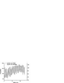
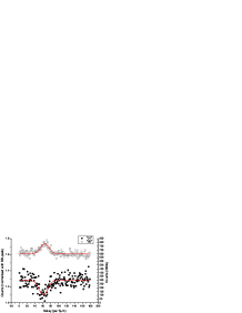
Figure 14: Left: The count rate for ‘01’ depends on the phases of the interferometers, which were not stabilized. Since this interference is single-photon interference it is present for both the main ‘01’-coincidence and for the baby-peaks. Right: Using the baby-peaks to normalize the main count rate it is possible to see a dip in the count rate when scanning an optical delay. This decrease is caused by photon bunching. The dip is in the same position as the measured antidip ‘00’.

If temporal alignment isn’t accomplished in a BS-BSA teleportation experiment the resulting coincidence rates will not depend on the phases of the interferometers and therefore a fringe with $V=0\%$ is found. When using an IF-BSA this is not the case since the presence of the extra interferometer leads to single photon interference when changing the phase $\alpha$. It is clearly important to be able to distinguish between these interferences and the interference fringes caused by teleportation. The behavior of the non-aligned setup can be readily calculated and the fringes that will be found are shown in Table 5. One important fact clearly stands out straight away: there is no interference for ‘02’ and ‘20’ if the photons are distinguishable but there is when the photons are indistinguishable. The visibility of these fringes are an important indication whether or not there was temporal alignment during the experiment. In the experiment presented here a visibility of $V=55\%\pm 3\%$ was found which indicates that there was temporal indistinguishability.

Other indications whether there is good temporal alignment can be found when simulating the result of an unaligned experiment. Such a simulation is shown (Fig. 15) for the case of $\delta=-\beta$ as was used during our experiments. The simulation clearly shows differences between the two cases which are readily identifiable in an experiment, such as the phaseshift of $\pi$ between the fringes for ‘01’ and ‘10’. These differences make it possible to see after an experiment whether or not the alignment was good and stayed good.

BSA	indistinguishable	distinguishable
‘01’	$1+cos(\alpha+\beta)$	$1+cos(\alpha)$
‘02’	$1-cos(\alpha+\beta)$	$1$
‘10’	$1+cos(\alpha+\beta)$	$3-cos(\alpha)$
‘11’	$4(1+cos(\alpha+\beta-2\delta))$	$2(2+2cos(\alpha-\delta))$
‘12’	$1+cos(\alpha+\beta)$	$3-cos(\alpha)$
‘20’	$1-cos(\alpha+\beta)$	$1$
‘21’	$1+cos(\alpha+\beta)$	$1+cos(\alpha)$

Table 5: Theoretical interference for different projections made by the BSA. Two different cases are shown: indistinguishable photons (teleportation) and distinguishable photons (noise).

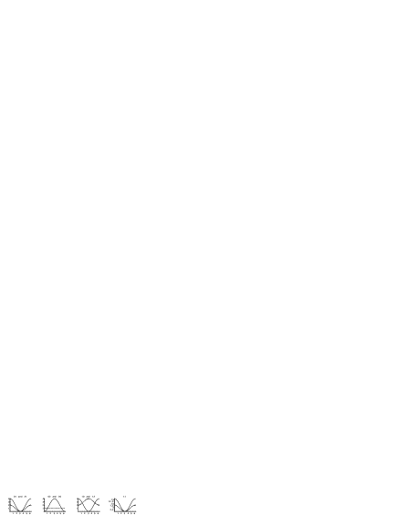
Figure 15: Simulation of result from a teleportation experiment in the case that the interferometers have been aligned to have $\delta=-\beta$ as was the case in our experiment. The dashed curves are for the case of distinguishable photons at the BSA and the plain curves are for indistinguishable photons (teleportation).

References

- (1) C. Bennett et al., Phys. Rev. lett. 70, 1895 (1993).
- (2) D. Bouwmeester et al., Nature 390, 575 (1997).
- (3) D. Boschi et al., Phys. Rev. Lett. 80, 1121 1125 (1998).
- (4) E. Waks, A. Zeevi, and Y. Yamamoto, Phys. Rev. A 65, 052310 (2002).
- (5) B. C. Jacobs, T. B. Pittman, and J. D. Franson, Phys. Rev. A 66, 052307 (2002).
- (6) I. Marcikic et al., Nature 421, 509 (2003).
- (7) D. Collins, N. Gisin, and H. De Riedmatten, Journal of Modern Optics 52, 735 (2005).
- (8) J.-W. Pan, D. Bouwmeester, H. Weinfurter, and A. Zeilinger, Phys. Rev. Lett. 80, 3891 (1998).
- (9) H. de Riedmatten et al., Phys. Rev. A 71, 050302(R) (2005).
- (10) C. H. Bennett and S. J. Wiesner, Phys. Rev. Lett. 69, 2881 (1992).
- (11) K. Mattle, H. Weinfurter, P. G. Kwiat, and A. Zeilinger, Phys. Rev. Lett. 76, 4656 (1996).
- (12) J. Calsamiglia and N. Lütkenhaus, Applied Physics B: Lasers and Optics 72, 67 (2001).
- (13) E. Knill, R. Laflamme, and G. Milburn, Nature 409, 46 (2001).
- (14) Y.-H. Kim, S. P. Kulik, and Y. Shih, Phys. Rev. Lett. 86, 1370 (2001).
- (15) S. L. Braunstein and H. J. Kimble, Phys. Rev. Lett. 80, 869 (1998).
- (16) A. Furusawa et al., Science 282, 706 (1998).
- (17) J. van Houwelingen et al., PRL 96, 130502 (2006).
- (18) H. Weinfurther, Europhysics Letters 25, 559 (1994).
- (19) P. Walther and A. Zeilinger, Phys. Rev. A 72, 010302(R) (2005).
- (20) W. Tittel, J. Brendel, N. Gisin, and H. Zbinden, Phys. Rev. A 59, 4150 (1999).
- (21) A. Einstein, B. Podolsky, and N. Rosen, Phys. Rev. 47, 777 (1935).
- (22) H. de Riedmatten et al., Phy. Rev. A 67, 022301 (2003).
- (23) H. de Riedmatten et al., Phys. Rev. Lett. 92, 047904 (2004).
- (24) V. Scarani, H. de Riedmatten, H. Marcikic, I.and Zbinden, and N. Gisin, Eur. Phys. J. D 32, 129 (2005).
- (25) W. Tittel and G. Weihs, QIC 1–56, 3 (2001).
- (26) J. D. Franson, Phys. Rev. Lett. 62, 2205 (1989).
- (27) C. K. Hong, Z. Y. Ou, and M. L., Phys. Rev. Lett. 59, 2044 (1987).
- (28) F. Grosshans and P. Grangier, Phys. Rev. A 64, 010301 (2001).
- (29) D. Bruss et al., Phys. Rev. A 57, 2368 (1998).