Dynamics of entanglement of bosonic modes on symmetric graphs
F. Ghahari,       V. Karimipour       R. Shahrokhshahi

Department of Physics, Sharif University of Technology,

P.O. Box 11365-9161,

Tehran, Iran

We investigate the dynamics of an initially disentangled Gaussian state on a general finite symmetric graph. As concrete examples we obtain properties of this dynamics on mean field graphs (also called fully connected or complete graphs) of arbitrary sizes. In the same way that chains can be used for transmitting entanglement by their natural dynamics, these graphs can be used to store entanglement. We also consider two kinds of regular polyhedron which show interesting features of entanglement sharing.

PACS Numbers: 03.67.-a, 03.65.Bz.

1 Introduction

One of the basic problems of quantum information processing is the problem of entanglement transformation or more generally manipulation of entanglement. For long distances one usually uses photons through optical fibres or free air to transmit entanglement . However for short distances other methods are being explored which are based on using discrete sets of interacting quantum systems such as spins [1, 2, 3, 4, 5] or harmonic oscillators [6], which by their natural dynamics can generate and transmit entanglement. In particular in [6], one dimensional lattices of harmonic oscillators coupled by two different types of Hamiltonians, were studied and various phenomena were investigated with regard to entanglement generation and transmission. Among other things it was shown that the largest amount of entanglement between two oscillators is always obtained when one places them at the two ends of an open chain. This maximality was attributed to the fact that in this case the two oscillators have fewer neighbors to which they can become entangled. It was argued in [6] that besides linear arrays of oscillators, other geometries, in principle any arrangement corresponding to weighted graphs are worth of study, since they can act as building blocks of more complicated networks. In [6] itself two other geometries, namely a $Y$ shape geometry which mimics a beam splitter and another geometry corresponding to an interferometer were studied.

In this article we want to extend these considerations in one particular direction, namely we want to study compact and symmetric geometries, i.e. symmetric graphs of finite size. The basic motivation is that in contrast to the geometries considered in [7, 8] which were suitable for transmission of entanglement, finite graphs are suitable for storing entanglement. As any other resource, entanglement needs to be stored for use in later suitable times and hence in any complicated network, building blocks which can store entanglement, should be implemented. In the simplest electrical analogy we may think of finite geometries as capacitors and linear arrays of the type considered in [6] as resistors or transmission lines.
However in contrast to the static properties of entanglement, for which various symmetric graphs have been considered [8], for our purpose, only one type of symmetric graph seems to be useful, namely the mean field or a fully connected graph. The reason is the very simple temporal behavior of entanglement on these graphs, compared with the complicated behavior of arbitrary graphs. In fact a system of harmonic oscillators on a mean field graphs has only two natural frequencies which makes the resulting time development of entanglement quite simple and easily controllable, while for other symmetric graphs, this is not the case. If as in [1] we are to extract entanglement at an optimal time, then it is of utmost importance that the dynamics of entanglement follows a simple and not a complicated pattern.

For that reason we mostly consider mean field clusters of arbitrary sizes and determine how an originally disentangled set of harmonic oscillators positioned on the nodes of such a cluster, when coupled to each other, develop a pairwise entanglement between themselves. How this entanglement develops in time, what is its maximum value, and how it depends on the size of the cluster. We stress that our general setting is apt for analysis of any symmetric graph and we indeed include two other graphs for observing some other phenomena.

The structure of this paper is as follows: In section 2 we briefly review the Gaussian states and their entanglement properties, especially we remind the closed formula for entanglement of Formation (EoF) [9] which in the context of symmetric graphs is more suitable than negativity as a measure of entanglement. In section 3 we study the dynamics of a Gaussian state on an arbitrary symmetric graph and obtain closed formulas for the EoF between any two sites as a function of time. This formula reduces the calculation of the EoF to the diagonalization of the adjacency matrix of the graph.
In section 4 we study in detail the simplest graph consisting of two nodes. In section 5 we specialize to the mean field graphs where our concrete results are reported in figures (2, 3, 4) and table (1).

Finally in section (6) we consider two other symmetric graphs for comparison and draw some conclusions about the sharing of entanglement which challenge the arguments of [6] on this issue.

2 Preliminaries on Gaussian States

In this section we collect the rudimentary material on Gaussian states that we need in the sequel. References [10, 11] can be consulted for rather detailed reviews on the subject of Gaussian states.
Let $\hat{R}:=(\hat{x}_{1},\hat{x}_{2},\cdots\hat{x}_{N},\hat{p}_{1},\hat{p}_{2},\cdots\hat{p}_{N})$ be $N$ conjugate operators characterizing $N$ modes and subject to the canonical commutation relations

$$[\hat{R}_{k},\hat{R}_{l}]=i\sigma_{kl},$$

where $\sigma=\left(\begin{array}[]{cc}&I_{n}\\ -I_{n}&\end{array}\right)$ is the $2n$ dimensional symplectic matrix and $I_{n}$ denotes the $n$ dimensional unit matrix.
A quantum state $\rho$ is called Gaussian if its characteristic function defined as $C(\xi):=tr(e^{-i\xi_{k}\sigma_{kl}\hat{R}_{l}}\rho),$ is a Gaussian function of the $\xi$ variables, namely if

$$C(\xi):=e^{\frac{-1}{2}\xi_{k}\Gamma_{kl}\xi_{l}},$$

where we have assumed that linear terms have been removed by suitable unitary transformations. The matrix $\Gamma$, called the covariance matrix of the state, encodes all the correlations in the form

$$\Gamma_{kl}:=\langle R_{k}R_{l}+R_{l}R_{k}\rangle-2\langle R_{k}\rangle\langle R_{l}\rangle.$$

For a two mode symmetric Gaussian state, one in which there is a symmetry with respect to the interchange of the two modes, the covariance matrix will be

$$\Gamma=\left(\begin{array}[]{cc}\alpha&\beta\\ \beta&\alpha\end{array}\right).$$ (1)

where the modes have been arranged in the order $x_{1},\ p_{1},\ x_{2},\ p_{2}$ and $\alpha$ and $\beta$ are $2\times 2$ symmetric matrices. By symplectic transformations the covariance matrix of a two mode symmetric Gaussian state can always be put into the standard form (in the order $x_{1},x_{2},p_{1},p_{2}$)

$$\Gamma_{s}=\left(\begin{array}[]{cccc}n&k_{x}&&\\ k_{x}&n&&\\ &&n&k_{p}\\ &&k_{p}&n\end{array}\right),$$ (2)

where $k_{x}\geq 0\geq k_{p}$ and $k_{x}\geq|k_{p}|$. The entries of the standard form of $\Gamma_{s}$ can be determined from the following symplectic invariants:

$$n^{2} = \det\alpha$$ (3)

$$k_{x}k_{p} = \det\beta$$ (4)

$$(n^{2}-k_{x}^{2})(n^{2}-k_{p}^{2}) = \det\Gamma.$$ (5)

For a symmetric Gaussian state a closed formula for the entanglement of Formation has been derived in [9]. Note that there are other criteria for studying the entanglement or separability of Gaussian states [12], however we use only Entanglement of Formation here to take advantage of the inherent built-in symmetry of our graphs. EoF of a Gaussian state $\rho$, denoted simply by $E(\rho)$ is expressed as follows:

$$E(\rho):=C_{+}\log_{2}C_{+}-C_{-}\log_{2}C_{-},$$ (6)

in which

$$C_{\pm}=\frac{(1\pm\Delta)^{2}}{4\Delta},$$ (7)

and

$$\Delta:=min(1,\delta:=\sqrt{(n-k_{x})(n+k_{p})}).$$ (8)

Thus a state is entangled only if $\delta\leq 1$.

Note that $\delta$ can be expressed in terms of the original covariance matrix. To express it we denote

$$u := \det\alpha$$ (9)

$$v := \det\beta$$ (10)

$$w := \det\Gamma$$ (11)

and

$$\xi:=u^{2}+v^{2}-w.$$ (12)

Then a simple calculation gives

$$\delta^{2}=u-v-\sqrt{\frac{\xi-\sqrt{\xi^{2}-4u^{2}v^{2}}}{2}}-\sqrt{\frac{\xi+\sqrt{\xi^{2}-4u^{2}v^{2}}}{2}}.$$ (13)

In the following sections we use this equation for calculating the entanglement of a Gaussian state which is initially disentangled and evolves in time under a quadratic hamiltonian.

3 Dynamics of entanglement of Gaussian states on symmetric graphs

Consider a symmetric graph, having $n$-nodes, corresponding to an adjacency matrix A and a system of bosonic modes corresponding to the vertices of this graph interacting by a quadratic Hamiltonian. In this paper we consider a Hamiltonian of the form

$$H=\frac{1}{2}\sum_{i=1}^{n}p_{i}^{2}+\frac{1}{2}\sum_{\langle i,j\rangle}x_{i}^{2}+x_{j}^{2}+c(x_{i}-x_{j})^{2},$$ (14)

where the sum runs over adjacent nodes and $c$ is a coupling constant. This Hamiltonian describes a simple mass-spring system of the form first studied by Plenio [6] in the context of entanglement dynamics. The above Hamiltonian can be written in the compact form

$$H=\frac{1}{2}R^{\dagger}\left(\begin{array}[]{cc}V&0\\ 0&T\end{array}\right)R$$ (15)

where $V$ and $T$ (here equal to I) are the potential and the kinetic matrices. We include the case of arbitrary $T$ (but commuting with $V$) for generality, since some other Hamiltonians like the one in [7] can be expressed in this way.

The dynamics of $R$ is easily determined by solving the equations of motion

$$\frac{dR}{dt}=-i[R,H]$$ (16)

or using $[R_{i},R_{j}]=i\sigma_{ij}$

$$\frac{dR}{dt}=\sigma\hat{H}R=\left(\begin{array}[]{cc}0&T\\ -V&0\end{array}\right)R.$$ (17)

The solution of the above equation is given by

$$R(t)=exp({\left(\begin{array}[]{cc}0&T\\ -V&0\end{array}\right)t})R(0).$$ (18)

The explicit form of the evolution matrix is found by writing it as

$$U(t):=exp({\left(\begin{array}[]{cc}0&T\\ -V&0\end{array}\right)t})=e^{\frac{1}{2}\sigma_{x}\otimes(T-V)+\frac{i}{2}\sigma_{y}\otimes(T+V)}.$$ (19)

In order to find the explicit form of the evolution matrix we use the following

Lemma: For any two commuting matrices $A$ and $B$, the following identity holds:

$$e^{A\otimes\sigma_{+}-B\otimes\sigma_{-}}=I\otimes\cos\sqrt{AB}+\left(\sigma_{+}\otimes\sqrt{\frac{A}{B}}-\sigma_{-}\otimes\sqrt{\frac{B}{A}}\right)\sin\sqrt{AB}.$$ (20)

This lemma is proved by a simple application of the identity $e^{i\theta\hat{n}\cdot\vec{\sigma}}=\cos\theta+i\sin\theta\hat{n}\cdot\vec{\sigma}$.

Using the above lemma, we find the final form of the evolution matrix

$$U(t) = I\otimes\cos\sqrt{VT}t+\left(\sqrt{\sigma_{+}\otimes\frac{T}{V}}-\sigma_{-}\otimes\sqrt{\frac{V}{T}}\right)\sin\sqrt{VT}$$ (21)

$$= \left(\begin{array}[]{cc}\cos\sqrt{VT}t&\sqrt{\frac{T}{V}}\sin\sqrt{VT}t\\ -\sqrt{\frac{V}{T}}\sin\sqrt{VT}t&\cos\sqrt{VT}t\end{array}\right)$$ (24)

For the case we consider in this article the kinetic matrix $T$ is identity ($T=I$) and so with the definition $W:=\sqrt{V}$, $U(t)$ simplifies to

$$U(t)=I\otimes\cos Wt+\left(\sigma_{+}\otimes W^{-1}-\sigma_{-}\otimes W\right)\sin Wt=\left(\begin{array}[]{cc}\cos Wt&W^{-1}\sin Wt\\ -W\sin Wt&\cos Wt\end{array}\right).$$ (25)

From the definition of the covariance matrix we find

$$\Gamma(t)=U(t)\Gamma(0)U^{T}(t).$$ (26)

Let us consider the case where the initial state is a completely uncorrelated state with $\Gamma(0)=I$.

The covariance matrix as a function of time will then be given by

$$\Gamma(t)=U(t)U^{T}(t)=\left(\begin{array}[]{cc}\cos^{2}Wt+W^{-2}\sin^{2}Wt&(W^{-1}-W)\sin Wt\cos Wt\\ (W^{-1}-W)\sin Wt\cos Wt&\cos^{2}Wt+W^{2}\sin Wt\end{array}\right).$$ (27)

The covariance matrix between any two modes (sites of the graph) is determined by extracting only the sub-matrix pertaining to those two sites. For this we need the matrix which diagonalizes $V$. Let $\Omega^{-1}W\Omega=W_{D}$ where $W_{D}$ is a diagonal matrices with diagonal elements $\omega_{i}$. The matrix $\Omega$ is the matrix which diagonalizes the adjacency matrix of the graph.

$$\Gamma(t)=(\Omega\oplus\Omega)\left(\begin{array}[]{cc}\Gamma_{xx}^{D}&\Gamma_{xp}^{D}\\ \Gamma_{xp}^{D}&\Gamma_{pp}^{D}\end{array}\right)(\Omega\oplus\Omega)^{T}$$ (28)

where

$$\Gamma_{xx}^{D} = diag\ \ (\cos^{2}\omega_{i}t+\omega_{i}^{-2}\sin^{2}\omega_{i}t)$$ (29)

$$\Gamma_{pp}^{D} = diag\ \ (\cos^{2}\omega_{i}t+\omega_{i}^{2}\sin^{2}\omega_{i}t)$$ (31)

$$\Gamma_{xp}^{D} = diag\ \ ((\omega_{i}^{-1}-\omega_{i})\sin\omega_{i}t\cos\omega_{i}t).$$ (33)

Then the covariance matrix between any two modes say modes $1$ and $2$ will be the form

$$\Gamma_{x_{1},x_{1}} = \Gamma_{x_{2},x_{2}}=\sum_{i=1}^{n}\Omega_{1i}^{2}({\Gamma_{xx}^{D}})_{i}$$ (34)

$$\Gamma_{x_{1},x_{2}} = \Gamma_{x_{2},x_{1}}=\sum_{i=1}^{n}\Omega_{1i}\Omega_{2i}({\Gamma_{xx}^{D}})_{i}$$ (35)

$$\Gamma_{p_{1},p_{1}} = \Gamma_{p_{2},p_{2}}=\sum_{i=1}^{n}{\Omega_{1i}}^{2}({\Gamma_{pp}^{D}})_{i}$$ (36)

$$\Gamma_{p_{1},p_{2}} = \Gamma_{p_{2},p_{1}}=\sum_{i=1}^{n}\Omega_{1i}\Omega_{2i}({\Gamma_{pp}^{D}})_{i}$$ (37)

$$\Gamma_{x_{1},p_{1}} = \Gamma_{x_{2},p_{2}}=\sum_{i=1}^{n}\Omega_{1i}^{2}({\Gamma_{xp}^{D}})_{i}$$ (38)

$$\Gamma_{x_{1},p_{2}} = \Gamma_{x_{2},p_{1}}=\sum_{i=1}^{n}\Omega_{1i}\Omega_{2i}({\Gamma_{xp}^{D}})_{i}.$$ (39)

Therefore in each case we should only determine the matrix $\Omega$ which diagonalizes the potential matrix $V$ and from (29, and 34 ) determine the eigenvalues $\omega_{i}$ . In the forthcoming sections we use this formalism to determine the dynamics of entanglement between any two modes on a wide variety of symmetric graphs. Note that the entanglement of formation is defined only for symmetric Gaussian states, and in this paper we are considering only symmetric graphs. So in all of the graphs that we consider, this entanglement is invariant under isomorphism of graphs.

4 The simplest example, A Two-Mode System

As the simplest example we consider a two mode system represented by a simple graph consisting of two nodes and a link connecting them.

The Hamiltonian is

$$H=\frac{1}{2}(p_{1}^{2}+p_{2}^{2})+\frac{1}{2}(x_{1}^{2}+x_{2}^{2}+c(x_{1}-x_{2})^{2}),$$ (40)

which corresponds to the matrices

$$T=I,\hskip 28.45274pt\ \ and\ \ V=\left(\begin{array}[]{cc}1+c&-c\\ -c&1+c\end{array}\right).$$ (41)

The eigenvalues of the matrix $V$ are readily obtained to be $1$ and $\omega:=\sqrt{1+2c}$.

The covariance matrix is given by

$$\Omega=\frac{1}{\sqrt{2}}\left(\begin{array}[]{cc}1&1\\ 1&-1\end{array}\right),$$ (42)

and

$$\Gamma^{D}_{x,x} = diag(1,\cos^{2}\omega t+\omega^{-2}\sin^{2}\omega t)$$ (43)

$$\Gamma^{D}_{p,p} = diag(1,\cos^{2}\omega t+\omega^{2}\sin^{2}\omega t)$$ (44)

$$\Gamma^{D}_{x,p} = diag(0,(\omega^{-1}-\omega)\sin\omega t\cos\omega t).$$ (45)

Using (13) we find the parameter $\delta$ which is essential for calculating the entanglement of the state. The result is

$$\delta=\sqrt{1+\frac{1}{4}(\omega^{-1}-\omega)^{2}\sin^{2}\omega t}-\frac{1}{2}\mid(\omega^{-1}-\omega)\sin\omega t\mid.$$ (46)

The entanglement of the state is shown in figure (1) for two difference coupling constants.

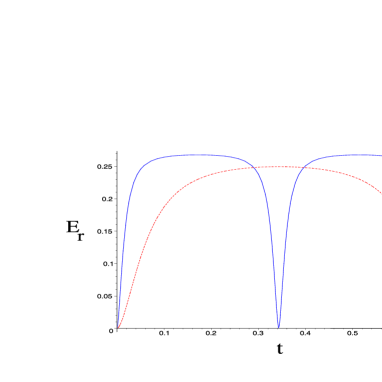
Figure 1: (color online) The entanglement between the two modes in a simple two-vertex graph, as a function of time, for two different couplings, $c=2$ (dashed line) and $c=8.3$ (solid line).

The entanglement oscillates at the natural frequency $\omega$. Its maximum value is achieved for the minimum value of $\delta$, or

$$\delta_{min}=\delta(\omega t=\frac{\pi}{2})=\sqrt{1+\frac{1}{4}(\omega^{-1}-\omega)^{2}}-\frac{1}{2}\mid(\omega^{-1}-\omega)\mid.$$

As we increase the frequency or the coupling constant, the entanglement becomes flat in most of the period and develops cusp singularities in half periods. Note that $\delta$ ranges between $0$ (for $\omega\longrightarrow\infty$) and $1$ (for $\omega=1$). Thus the maximum entanglement increases unboundedly by increasing the strength of the interaction $c$. In fact the maximum entanglement increases as $\log\ \omega$ for large coupling constants $c$.
Thus a two-vertex graph can be used as a storage device for entanglement the ”capacity” of which increases logarithmically with the coupling constant $c$. Moreover as the flatness of the curve in figure (1) shows, for very large coupling constants we can extract this maximum entanglement at any time we wish except for a discrete set of points.

5 Mean Field Clusters

We now consider a mean field cluster of $N$ vertices in which every vertex is connected to $N-1$ other vertices. The adjacency matrix for a mean field graph is given by

$$\hat{{\bf A}}=E-I,$$ (47)

where $E$ is the matrix all of whose entries are equal to 1, $E_{ij}=1\ \ \ \forall\ \ \ i,\ \$ and $\ j$. The potential matrix of this graph is given by

$$\hat{V}=(1+Nc)I-cE.$$ (48)

The matrix $E$ and hence ${\bf V}$ can easily be diagonalized. We have

$$Ee_{0}=Ne_{0},\hskip 28.45274ptEe_{k}=0,\ \ \ k=1,2,\cdots N-1,$$ (49)

where

$$e_{0} = \frac{1}{\sqrt{N}}(1,1,\cdots 1)^{T},$$ (50)

$$e_{k} = \frac{1}{\sqrt{k(k+1)}}(1,1,1,\cdots-k,\cdots 0)^{T},\ \ \ \ k=1,2,\cdots N-1.$$ (51)

Thus the eigenvalues of ${\bf V}$ will be given by

$$\omega_{0}=1\hskip 28.45274pt\omega_{1}=\cdots\omega_{N-1}=\sqrt{1+Nc}=:\omega.$$ (52)

The eigenvectors $e_{0}$ to $e_{N-1}$ derived above easily yield the diagonlizing matrix $\Omega$ ($\Omega_{ij}=(e_{j})_{i}$) from which we can obtain after straightforward calculations from (29) and (34) the following parameters of the covariance matrix between any two sites say sites $1$ and $2$:

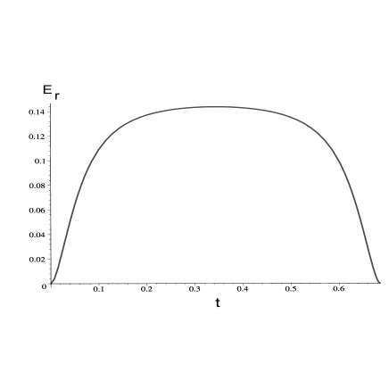
Figure 2: The re-scaled entanglement as a function of time for a mean field cluster of size $N=20$ at $c=1$, the time spans one full period.

$$\Gamma_{x_{1},x_{1}} = \Gamma_{x_{2},x_{2}}=\frac{1}{N}+(1-\frac{1}{N})(\cos^{2}\omega t+\omega^{-2}\sin^{2}\omega t)$$ (53)

$$\Gamma_{x_{1},x_{2}} = \Gamma_{x_{2},x_{1}}=\frac{1}{N}(1-\omega^{-2})\sin^{2}\omega t$$ (54)

$$\Gamma_{p_{1},p_{1}} = \Gamma_{p_{2},p_{2}}=\frac{1}{N}+(1-\frac{1}{N})(\cos^{2}\omega t+\omega^{2}\sin^{2}\omega t)$$ (55)

$$\Gamma_{p_{1},p_{2}} = \Gamma_{p_{2},p_{1}}=\frac{1}{N}(1-\omega^{2})\sin^{2}\omega t$$ (56)

$$\Gamma_{x_{1},p_{1}} = \Gamma_{x_{2},p_{2}}=(1-\frac{1}{N})(\omega^{-1}-\omega)\sin\omega t\cos\omega t$$ (57)

$$\Gamma_{x_{1},p_{2}} = \Gamma_{x_{2},p_{1}}=-\frac{1}{N}(\omega^{-1}-\omega)\sin\omega t\cos\omega t$$ (58)

One can obtain the standard form of this matrix by using the symplectic invariants. They read in the present case

$$u = \ 1+\frac{1}{N}(1-\frac{1}{N})(\omega-\omega^{-1})^{2}\sin^{2}\omega t,$$ (59)

$$v = \ \frac{-1}{N^{2}}(\omega-\omega^{-1})^{2}\sin^{2}\omega t,$$ (60)

$$w = \ 1+2(\omega-\omega^{-1})^{2}(\frac{N-2}{N^{2}})\sin^{2}\omega t.$$ (61)

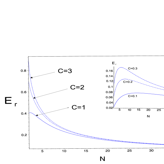
Figure 3: The maximum re-scaled EoF for mean field clusters for different coupling constants.

Inserting these values in 13 gives the entanglement for these graphs. Following [13], we define re-scaled entanglement $(E_{r})$ which is $N-1$ times the entanglement between any two nodes. This definition stems from the fact that a node shares its entanglement with its neighbors which are $N-1$ in number.
Figure (2) shows the re-scaled entanglement for a mean field cluster of size 20 as a function of time. Figure (3) show the maximum re-scaled entanglement for mean field clusters as a function of their size for different coupling constants.

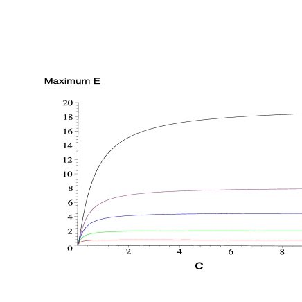
Figure 4: The amplitude of oscillation of entanglement ($E$) in units of 0.01 ebits, for mean field clusters of different sizes as a function of coupling constant. The saturation values are always less than the bounds found in [7]. Note that for all the sizes $N>2$, as $c$ increases, $E$ saturates to finite values.

For any cluster of size $N$ and coupling constant $c$, the entanglement oscillates at a frequency $\omega:=2\sqrt{1+Nc}$ and most of the time the two modes have an appreciable amount of entanglement. With increasing the coupling constant $c$, the amplitude of oscillation increases and saturates to a finite value for very large $c$, as long as $N>2$ (figure 4). Table (1) shows this saturated amplitude for clusters of different sizes.

N	Maximum $E_{r}$
2	$\infty$
3	$0.803$
4	$0.592$
5	$0.484$
6	$0.415$
7	$0.365$
8	$0.328$
9	$0.298$
10	$0.274$
15	$0.196$
20	$0.156$
30	$0.113$

Table 1: The saturated amplitude of re-scaled entanglement for mean field graphs of different sizes.

6 Sharing of entanglement

As mentioned in the introduction, in [6] it was shown that in a linear lattice, the largest amount of entanglement between pairs of sites with the same distance, occurs when these two sites are at the end points of the lattice. This was attributed to the fact that the endpoints of the lattice have fewer neighbors to which they share their entanglement. In this regard it is instructive to consider two symmetric graphs which are not fully connected. The two graphs which we study are a six-vertex graph in the shape of octahedron and an eight-vertex graph in the shape of a cube. They are shown in figure (5) with numbered vertices.

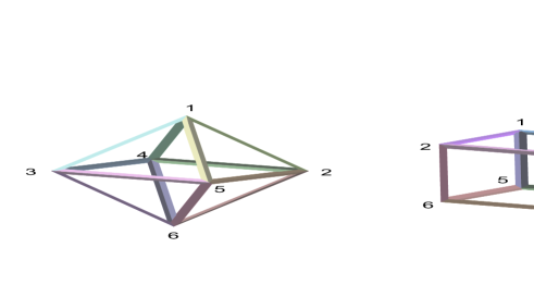
Figure 5: (color online) Two symmetric graphs, Cube and the Octahedron, the entanglement between different pairs of vertices are plotted in figure figure 6 and 7.

In the octahedron there are essentially two types of pairs, represented by the pair (1,2) and the pair (1,6). In each pair the number of neighbors of each node is the same. However the pair (1,6) although more apart than the pair (1,2) develops a much higher entanglement, figure 6.

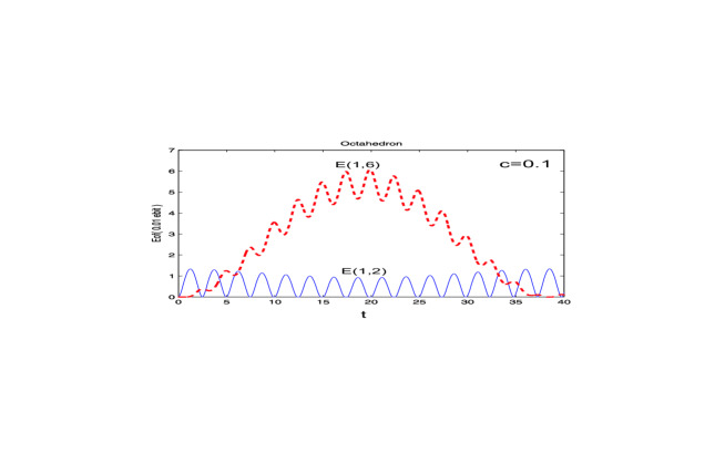
Figure 6: (color online) The pairwise entanglement between the sites $(1,2)$ and the sites $(1,6)$ in the Octahedron as a function of time.

In terms of the number of edges, the distance between the nodes 1 and 2 is one, and there is only one shortest path which connects these two nodes, while the distance between nodes 1 and 6 is two, however there are four such shortest paths which connect these two nodes. Therefore it seems that entanglement between two site is not only affected by the number of their neighbors, but also by the number of shortest paths which connects these two sites to each other. To test this idea, we study the cube, which has three types of pairs represented by the (1,2), (1,6) and (1,7), with distances respectively given by 1, 2 and 3 and the number of shortest paths respectively given by 1, 2, and 6. The entanglement is shown in figure (7) which confirms our assertion. Here we see a competition between the two factors.

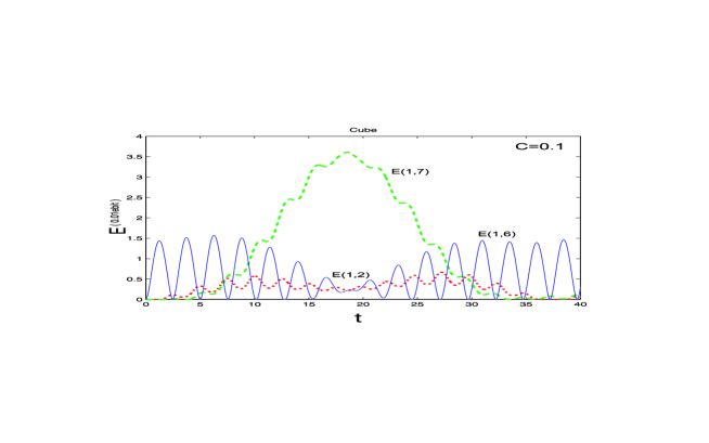
Figure 7: (color online) The pairwise entanglement between the sites $(1,2)$, $(1,3)$ and $(1,6)$ in the Cube as a function of time.

If we interpret the entanglement as a direct measure of quantum correlations then these two figures show a very intriguing property of entanglement: there are times where remote sites are strongly quantum correlated while the nearest sites have a small quantum correlation.

7 Acknowledgements

We would like to thank the members of the Quantum information group of Sharif University for very valuable comments.

References

- [1] S. Bose, Phys. Rev. Letts. 91, 20791 (2003).
- [2] C. Hadley, A. Serafini, and S. Bose, Phys. Rev. A 72, 052333 (2005).
- [3] J. Eisert, M.B. Plenio, S. Bose, and J. Hartley, Phys. Rev. Lett. 93, 190402 (2004).
- [4] A. Bayat, and V. Karimipour, Phys. Rev. A 71, 042330 (2005).
- [5] M. Christandl et al, Phys. Rev. A., 032312(2005).
- [6] M.B. Plenio, J. Hartley, and J. Eisert, New J. Phys. 6, 36 (2004).
- [7] M.M. Wolf, F. Verstraete, and J.I. Cirac, Phys. Rev. Lett. 92, 087903 (2004).
- [8] M. Asoudeh and V. Karimipour, Phys. Rev. A, 72, 0332339 (2005).
- [9] G. Giedke, M. M. Wolf, O. Kr ger, R. F. Werner, and J. I. Cirac, Phys. Rev. Lett. 91, 107901 (2003).
- [10] B. Englert and K. Wodkiewicz, Int. Jour. Quant. Information, vol 1, No. 2, (2003) 153-188.
- [11] A. Ferraro, S. Olivares, and M. G. A. Paris, ”Gaussian states in continuous variable quantum information”, quant-ph/0503237.
- [12] S. Mancini and S. Severini, ”The quantum separability problem for Gaussian States”, eprint, cs.CC/0603047.
- [13] J. Vidal, G. Palacios, and R. Mosseri, Phys. Rev. A 69, 022107 (2004).