Thermal Entanglement in Ferrimagnetic Chains

Abstract

A formula to evaluate the entanglement in an one-dimensional ferrimagnetic system is derived. Based on the formula, we find that the thermal entanglement in a small size spin-1/2 and spin-$s$ ferrimagnetic chain is rather robust against temperature, and the threshold temperature may be arbitrarily high when $s$ is sufficiently large. This intriguing result answers unambiguously a fundamental question: “can entanglement and quantum behavior in physical systems survive at arbitrary high temperatures?”

A physical system may exhibit entanglement at a finite temperature M_Nielsen ; M_Arnesen ; M_Wang01 ; M_Gunlycke ; Vedral . The thermal entanglement always vanishes above a threshold temperature for systems with finite Hilbert space dimension Fine . Recently, Ferreira et al. raised a fundamental question: can entanglement and quantum behavior in physical systems survive at arbitrary high temperatures? Ferreira They found that the entanglement between a cavity mode and a movable mirror does occur for any finite temperature. This result sheds a new light on the question and help to understand macroscopic properties of solids.

In this report, we derive a formula to evaluate the entanglement in an one-dimensional ferrimagnetic system. Intriguingly, we find that the entanglement is rather robust against temperature in this kind of system, with the Hamiltonian

$$H=J\sum_{n}({\bf s}_{n}\cdot{\bf S}_{n+1}+{\bf S}_{n+1}\cdot{\bf s}_{n+2}),$$ (1)

where ${\bf s}_{n}$ and ${\bf S}_{n}$ are spin-1/2 and spin-$s$ operators, respectively. The antiferromagnetic exchange interactions exist only between nearest neighbors, and they are of the same strength which is set to unity $(J=1)$. Physically, the system contains two kinds of spins, spin $\frac{1}{2}$ and $s$, alternating on a ring (or a chain with the periodic boundary condition).

Let us now study the entanglement of states of the system at thermal equilibrium described by the density operator $\rho(T)=\exp(-\beta H)/Z$, where $\beta=1/k_{B}T$, $k_{B}$ is the Boltzmann’s constant, which is assume to be 1, and $Z=\text{Tr}\{\exp(-\beta H)\}$ is the partition function. The entanglement in the thermal state is referred to as the thermal entanglement.

To study quantum entanglement in the ferrimagnetic system, we need a good entanglement measure. One possible way is to use the negativity Vidal based on the partial transpose method PH . In the cases of two spin halves and the (1/2,1) mixed spins, a positive partial transpose (PPT) (or the non-zero negativity) is necessary and sufficient for separability (entanglement). Although the present ferrimagnetic system is a kind of (1/2,$s$) system, fortunately, it was shown that due to the SU(2) symmetry in the model Hamiltonian (1), the non-zero negativity is still a necessary and sufficient condition for entanglement between a spin half and spin $s$ Schliemann . This result allows us to exactly investigate entanglement features of our mixed spin systems.

The negativity of a state $\rho$ is defined as

$${\cal N(\rho)}=\sum_{i}|\mu_{i}|,$$ (2)

where $\mu_{i}$ is the negative eigenvalue of $\rho^{T_{2}}$, and $T_{2}$ denotes
the partial transpose with respect to the second system. The negativity ${\cal N}$ is related to the trace norm of $\rho^{T_{2}}$ via

$${\cal N(\rho)}=\frac{\|\rho^{T_{2}}\|_{1}-1}{2},$$ (3)

where the trace norm of $\rho^{T_{2}}$ is equal to the sum of the absolute values of the eigenvalues of $\rho^{T_{2}}$.

Obviously, our system has the SU(2) symmetry, and any two-spin reduced density matrix from the thermal state is also SU(2)-invariant. Now, we consider the entanglement between the spin half and spin $s$, and derive the corresponding expression of negativity by the partial time reversal method breuer , which is equivalent to the partial transpose method up to a local unitary operator.

The density matrix of an SU(2)-invariant state for the spin half and spin $s$ can be written in the form

$$\rho=\frac{F}{2s}{\bf P}_{s-1/2}+\frac{1-F}{2s+2}{\bf P}_{s+1/2}$$ (4)

with $F\in[0,1]$. One may immediately check that the parameter $F$ is identical to the expectation value of the projector ${\bf P}_{s-1/2}$ on the densitry matrix, i.e., $F=\langle{\bf P}_{s-1/2}\rangle$. Noting the fact that ${\bf P}_{s-1/2}+{\bf P}_{s+1/2}=1$, we rewrite the density operator as

$$\rho=\frac{(2sF+F-s){\bf P}_{s-1/2}}{2s(s+1)}+\frac{1-F}{2s+2}.$$ (5)

and obtain the relations

$${\bf P}_{s-1/2}= \frac{1}{2s+1}(s-2\mathbf{s}_{1}\cdot\mathbf{S}_{2})$$

$${\bf P}_{s+1/2}= \frac{1}{2s+1}(s+1+2\mathbf{s}_{1}\cdot\mathbf{S}_{2}).$$ (6)

The partial time reversal operator $\tau_{2}$ changes the sign of ${\bf S}_{2}$ and ${\bf s}_{1}\cdot{\bf S}_{2}$

$$\tau_{2}({\bf S}_{2})= -{\bf S}_{2}$$

$$\tau_{2}({\bf s}_{1}\cdot{\bf S}_{2})= -{\bf s}_{1}\cdot{\bf S}_{2},$$ (7)

Therefore, we get

$$\tau_{2}({\bf P}_{s-1/2})=\frac{2s}{2s+1}-{\bf P}_{s-1/2}.$$ (8)

We see that the partial time reversal also changes the sign of projector, but with an additional additive constant.

Using Eqs. (5) and (8), the partial time reversed density matrix is obtained as

$$\rho^{\tau_{2}}=-\frac{(2sF+F-s){\bf P}_{s-1/2}}{2s(s+1)}+\frac{2sF+F+1}{2(2s+1)(s+1)}.$$ (9)

Any projector has two eigenvalues 0 and 1. Thus, from the above equation, we deduce that only the following eigenvalue of $\rho^{\tau_{2}}$ is possibly negative

$$\lambda= \frac{1}{2s+1}-\frac{F}{2s}$$

$$= \frac{1}{2s+1}\left(\frac{1}{2}+\frac{1}{s}\langle{\bf s}_{1}\cdot{\bf S}_{2}\rangle\right),$$ (10)

where we have used the first equality in Eq. (Thermal Entanglement in Ferrimagnetic Chains). By taking into account that the eigenvalue occurs with multiplicity $2s$, we finally obtain the negativity

$$\mathcal{N}=\max\left[0,-\frac{s+2\langle\mathbf{s}_{1}\cdot\mathbf{S}_{2}\rangle}{2s+1}\right].$$ (11)

The negativity is only determined by a single correlator, which is due to the fact that our state is SU(2)-invariant.

At this stage, to obtain straightforwardly analytical results of negativity in the present ferrimagnetic system as well as to gain some essential physical insight into entanglement features like the intriguing high-temperature entanglement, we here focus only on a two-spin case first. In this case, the Heisenberg interaction can be written in terms of projectors as follows

$$H=\mathbf{s}_{1}\cdot\mathbf{S}_{2}= \frac{1}{2}[(\mathbf{s}_{1}+\mathbf{S}_{2})^{2}-\mathbf{s}_{1}^{2}-\mathbf{S}_{2}^{2}]$$

$$= \frac{1}{2}(\mathbf{s}_{1}+\mathbf{S}_{2})^{2}-\frac{3}{8}-\frac{s(s+1)}{2}$$

$$= -\frac{s+1}{2}{\bf P}_{s-1/2}+\frac{s}{2}{\bf P}_{s+1/2}.$$ (12)

From Eq. (Thermal Entanglement in Ferrimagnetic Chains), the eigenvalues are simply

$$E_{0}=-\frac{s+1}{2},E_{1}=\frac{s}{2}.$$ (13)

The eigenvalue is just the expectation value of the correlator $\langle{\bf s}_{1}\cdot{\bf S}_{2}\rangle$ in the corresponding state. From Eqs. (13) and (11), the negativity for the ground state and the first excited state are obtained as

$$\mathcal{N}_{0}=\frac{1}{2s+1},\;\mathcal{N}_{1}=0.$$ (14)

Clearly, the ground-state is entangled, while the first-excited state is not. In addition, we observe that the ground-state entanglement decreases as $s$ increases, and finally vanishes in the limit of $s=\infty$. Note that, the case of $s=\infty$ corresponds actually to a classical spin, and thus, as expected intuitively, there exists no entanglement between a quantum system and a classical one indeed.

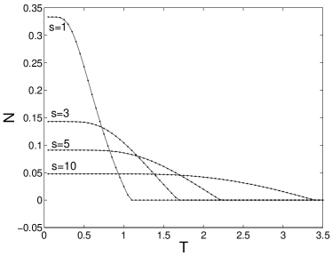
Figure 1: Negativity versus temperature for different $s$ in the two-site system.

At finite temperatures, we need to know the correlator $\langle\mathbf{s}_{1}\cdot\mathbf{S}_{2}\rangle$ evaluated on the thermal state, which completely determines the negativity. From Eq. (13), we obtain readily the partition function and the correlator as

$$Z=2se^{\frac{(s+1)\beta}{2}}+2(s+1)e^{-\frac{s\beta}{2}}$$ (15)

and

$$\langle\mathbf{s}_{1}\cdot\mathbf{S}_{2}\rangle=-\frac{1}{Z}\frac{\partial Z}{\partial\beta}=-\frac{s(s+1)}{Z}\left(e^{\frac{{s+1}\beta}{2}}-e^{-\frac{s\beta}{2}}\right).$$ (16)

Substituting Eqs. (16) and (15) into Eq. (11), the negativity is explicitly expressed as

$${\cal N}=\frac{2s}{(2s+1)Z}\max\{0,e^{\frac{(s+1)\beta}{2}}-2(s+1)e^{-\frac{s\beta}{2}}\}$$ (17)

The numerical results of negativity versus temperature for different $s$ are plotted in Fig. 1. As expected, for a fixed $s$, the negativity decreases monotonically as temperature increases, and vanishes when the temperature is equal or larger than a threshold value $T_{\text{th}}$. But more arrestingly, when $s$ is large, the entanglement is rather robust against temperature.

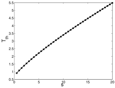
Figure 2: Threshold temperature versus $s$.

From Eq. (17), the threshold value of the thermal entanglement is found to be

$$T_{\text{th}}=\frac{2s+1}{2\ln(2s+2)},$$ (18)

from which we immediately have a striking result

$$\lim_{s\rightarrow\infty}T_{\text{th}}=\infty.$$ (19)

The threshold temperature $T_{\text{th}}$ can be arbitrarily high when $s$ is large enough. A plot of $T_{\text{th}}$ versus $s$ is illustrated in Fig. 2, and we observe that the threshold temperature increases with the increase of $s$.

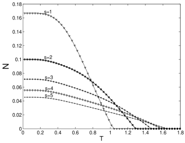
Figure 3: Negativity versus temperature for different $s$ in the four-site system.

It is now interesting to estimate some typical values in terms of Eq. (18) (with the unit $J/k_{B}$). The value of exchange constant $J$ is of the order $meV$. For a temperature $T\sim 127K$, the corresponding $s$ is estimated as $s=50$, above which the thermal entanglement exists. In this case, the negativity is approximately 0.01 at temperatures well below the above temperature.

Finally, we wish to address briefly the negativity of the systems with a larger number of sites $L$. For the four-site case, we can still have exact results and plot the negativity versus temperature for different $s$ in Fig. 3. It is seen that the negativity behaviors of the four-site case are qualitatively the same as those of the two-site case, namely, when $s$ increases, the negativity at zero temperature decreases and the threshold temperature increases. As for even larger sizes $L=2N$, due to the limitation of computational resource, we here can only make a qualitative analysis with the help of an approximate analytical result for the ground state energy obtained from the spin-wave theory Pati . At zero temperature, the nearest spin correlator Pati $\langle\mathbf{s}_{1}\cdot\mathbf{S}_{2}\rangle_{0}=E_{0}(L)/2L=-s/2-\delta(s)$, where the subscript index $0$ denotes the ground state, and $\delta(s)>0$ and approaches (1/4) in the limit $s\rightarrow\infty$. Therefore, from Eq.(11), the negativity $\mathcal{N}=2\delta(s)/(2s+1)$ is non-zero at zero temperature. Also, for a small size chain, we note that there exists a energy gap (proportional to $s$) between the excited and ground states, so the negativity is mainly determined by the ground state contribution at finite temperatures well below the gap energy, and may be non-zero at high temperature for a very large $s$.

In conclusion, by considering a simple ferrimagnetic chain model, we have found that the entanglement is rather robust against temperature. As the spin $s$ increases, the threshold temperature for entanglement can be arbitrarily high for a small size chain. We hope that the present work motivates interests to investigate other physical systems which display high-temperature entanglement.

- (1) M. A. Nielsen, Ph. D thesis, University of Mexico, 1998, quant-ph/0011036.
- (2) M. C. Arnesen, S. Bose, and V. Vedral, Phys. Rev. Lett. 87, 017901 (2001).
- (3) X. Wang, Phys. Rev. A 64, 012313 (2001); Phys. Lett. A,281, 101 (2001).
- (4) D. Gunlycke, V. M. Kendon, V. Vedral, and S. Bose, Phys. Rev. A64, 042302 (2001).
- (5) V. Vedral, New J. Phys. 6, 102 (2004).
- (6) V. Fine, F. Mintert, and A. Buchleitner, Phys. Rev. B 71, 153105 (2005).
- (7) A. Ferreira, A. Guerreiro, and V. Vedral, quant-ph/0504186.
- (8) G. Vidal and R. F. Werner, Phys. Rev. A65, 032314 (2002).
- (9) A. Peres, Phys. Rev. Lett. 77, 1413 (1996); M. Horodecki, P. Horodecki, and R. Horodecki, Phys. Lett. A 223, 1 (1996).
- (10) J. Schliemann, Phys. Rev. A68, 012309 (2003).
- (11) H. P. Breuer, Phys. Rev. A 71, 062330 (2005).
- (12) S. K. Pati, S. Ramaseha, and D. Sen, Phys. Rev. B 55, 8894 (1997).