Quantum criticality in a generalized Dicke model

Abstract

We employ a generalized Dicke model to study theoretically the quantum criticality of an extended two-level atomic ensemble interacting with a single-mode quantized light field. Effective Hamiltonians are derived and digonalized to investigate numerically their eigenfrequencies for different quantum phases in the system. Based on the analysis of the eigenfrequencies, an intriguing quantum phase transition from a normal phase to a super-radiant phase is revealed clearly, which is quite different from that observed with a standard Dicke model.

I Introduction

Quantum phase transition (QPT) and quantum critical phenomena, which are induced by the change of parameters and are accompanied by a dramatic change of physical properties, occur at zero temperature in many-body quantum systems sachev . Usually, a QPT may emerge in the parameter region where there is the energy level crossing or the symmetry-breaking. QPTs have been mainly studied in connection with correlated electron and spin systems in condensed matter physics sachev . Very recently, it has also been paid much attention in the light-atoms interacting systems Reslen05 ; emary , which enables us to understand the transition from radiation to super-radiation from a different viewpoint.

The systems of atomic ensembles interacting with optical fields have been studied both experimentally and theoretically, e.g., the electromagnetic induced transparency Harris and the quantum storage of photon states lukin ; sun-li-liu-prl . The thermal phase transition phenomena Rzazewski have been studied in the Dicke model Dicke54 (that is, a two-level atomic ensemble coupling with optical field) or generalized Dicke models Hioe . In particular, the QPT in a radiation-matter interacting system was recently explored based on the Dicke model, but merely with the single-mode Dicke model Reslen05 ; emary ; emary2 ; Vidal . When the coupling parameter $\lambda$ varies from that less than the critical value $\lambda_{c}$ to that larger than $\lambda_{c}$, the system goes from the normal phase to the super-radiant one in the presence of the symmetry-breaking. As the precursors of the QPT, the onset of chaos emary and the entanglement properties emary2 were studied in detail. However, it is noticed that these studies focused only on atomic ensembles with small dimensions compared with the optical wavelength, in which the dipole approximation can be used Reslen05 ; emary ; emary2 . In this special case, the light-atoms interaction is irrelevant to the spatial positions of atoms. But, generally speaking, a realistic atomic ensemble may extend in a large scale so that light-atoms interaction is spatially dependent Dicke54 ; scully06 .

In this paper, an exotic QPT phenomenon is investigated theoretically by developing the Dicke model for a more general case beyond the dipole approximation. We find that a kind of quantum critical phenomenon also occurs in this extended atomic ensemble, in which each atom interacts with a single mode quantized light field; but the quantum criticality is quite different from that deduced from the spatially independent Dicke model emary . In the present study, a normal phase and four possible super-radiant phases are found, with only one of the four exhibiting the same critical point as that in the normal phase. Remarkably, it is shown that the ground-state energy in the above-mentioned superradiant phase, connects continuously to the normal phase one at the critical point, but its second drivative does not.

II A generalized Dicke model for an extended atomic ensemble

Let us consider an extended ensemble with $N$ identical two-level atoms interacting with a single-mode quantized light field. Here, the spatial dimension of the atomic ensemble is much larger than the optical wavelength of the field. This radiation-matter system is usually described by a generalized Dicke model Dicke54 with the Hamiltonian $H=H_{0}+H_{I}$,

$$H_{0} = \omega a^{\dagger}a+\omega_{0}\sum_{j=1}^{N}\sigma_{\mathrm{ee}}^{(j)},$$

$$H_{I} = \frac{\lambda}{\sqrt{N}}\sum_{j=1}^{N}(a^{\dagger}\mathrm{e}^{-ikr_{j}}+a\mathrm{e}^{ikr_{j}})(\sigma_{\mathrm{eg}}^{(j)}+\sigma_{\mathrm{ge}}^{(j)}).$$ (1)

Here, $\hbar=1$, $k$ is the wave vector of the quantized light field and $r_{j}$ is the position of $j$th atom; $\sigma_{\mathrm{ee}}^{(j)}$ is the population operator of the $j$ atom; $\sigma_{\mathrm{eg}}^{(j)}$ is the flip operators between the excited state $\left|e\right\rangle$ and ground state $\left|g\right\rangle$ of the $j$ atom with the same energy differences $\omega_{0}$ for all the atoms; $a$ ($a^{\dagger}$) is the annihilation (creation) operator of the quantized light field, with $\lambda$ the relative coupling parameter. For simplicity, the ensemble is assumed to be one-dimensional with its direction along the wave vector.

Different from a standard Dicke model for small-dimension atomic ensembles emary , the spatial-dependent factors $\exp(\pm ikr_{j})$ are taken into account seriously though the momentum of the center of mass can be neglected. It is also remarked that the terms connected to the nonrotating-wave scenario are still kept in Hamiltonian (1); in fact, if the rotating-wave approximation were used, the factors $\exp(\pm ikr_{j})$ would be absorbed into $\sigma_{\mathrm{eg}}^{(j)}$ and $\sigma_{\mathrm{ge}}^{(j)}$ Fleischhauer05 ; Li05 .

III Normal phase

We can first introduce the following collective operators sun-li-liu-prl :

$$B^{\dagger} = \frac{1}{\sqrt{N}}\sum_{j=1}^{N}\sigma_{\mathrm{eg}}^{(j)}\mathrm{e}^{ikr_{j}},\text{ }$$

$$C^{\dagger} = \frac{1}{\sqrt{N}}\sum_{j=1}^{N}\sigma_{\mathrm{eg}}^{(j)}\mathrm{e}^{-ikr_{j}}.$$ (2)

It is obvious that in the limit of large $N$ with a small number of excitations (referred to as the normal phase), namely, the excitation numbers in states $\left|e\right\rangle$ are much less than $N$, the above two operators approximately satisfy the independent bosonic commutation relations

$$\left[B,B^{\dagger}\right]\approx\left[C,C^{\dagger}\right]\approx 1,\text{ \ }\left[B,C^{\dagger}\right]\approx 0$$ (3)

in the present extended ensemble, and can approximately be re-expressed as the two independent Bose operators $b^{\dagger}$ and $c^{\dagger}$

$$\left[b,b^{\dagger}\right]=\left[c,c^{\dagger}\right]=1,\text{ \ }\left[b,c^{\dagger}\right]=0.$$ (4)

In the present normal phase case, the original radiation-matter system described by Eq. (1) is approximated as a coupling three-mode bosonic system with the “low energy” effective Hamiltonian

$$H^{(n)} = \omega_{0}(b^{\dagger}b+c^{\dagger}c)+\omega a^{\dagger}a$$

$$+\lambda a^{\dagger}(c^{\dagger}+b)+\text{H.c.}.$$

We now apply a Bogoliubov transformation to diagonalize the above quadratic Hamiltonian (III) book . First, we rewrite it as

$$H^{(n)}=\frac{1}{2}\mathrm{U}^{(n)\dagger}M^{(n)}\mathrm{U}^{(n)}-\frac{1}{2}\mathrm{tr}\text{ }A^{(n)},$$ (6)

where the operator-valued vectors $\mathrm{U}^{(n)}$ and the matrices $M^{(n)}$, $A^{(n)}$, $B^{(n)}$ are defined as

$$\mathrm{U}^{(n)} = \left(a,b,c;a^{\dagger},b^{\dagger},c^{\dagger}\right)^{T},$$

$$M^{(n)} = \left(\begin{array}[]{cc}A^{(n)}&B^{(n)}\\ B^{(n)\ast}&A^{(n)\ast}\end{array}\right),$$ (9)

$$A^{(n)} = \left(\begin{array}[]{ccc}\omega&\lambda&0\\ \lambda&\omega_{0}&0\\ 0&0&\omega_{0}\end{array}\right),$$ (13)

$$B^{(n)} = \left(\begin{array}[]{ccc}0&0&\lambda\\ 0&0&0\\ \lambda&0&0\end{array}\right).$$ (17)

According to Ref. book , we diagonalize the Hamiltonian (6) in two steps: (i) find a unitary canonical transformation $T^{(n)}$ such that $T^{(n)}\hat{\eta}T^{(n)\dagger}\hat{\eta}=1$, $T^{(n)\ast}=\hat{\gamma}T^{(n)}\hat{\gamma}$, where

$$\hat{\eta}=\left(\begin{array}[]{cc}1&0\\ 0&-1\end{array}\right),\text{ \ }\hat{\gamma}=\left(\begin{array}[]{cc}0&1\\ 1&0\end{array}\right);$$ (18)

and (ii) introduce the quasiparticle operators

$$\mathrm{V}^{(n)}=T^{(n)}\mathrm{U}^{(n)}=(h_{1},h_{2},h_{3};h_{1}^{\dagger},h_{2}^{\dagger},h_{3}^{\dagger})^{T}.$$

Then the Hamiltonian (6) is cast into a diagonalized form

$$H^{(n)}=\sum_{i=1}^{3}\omega_{i}^{(n)}(h_{i}^{\dagger}h_{i}+\frac{1}{2})-\frac{1}{2}\mathrm{tr}A^{(n)},$$ (19)

and describes the quasiparticle excitations with frequencies $\omega_{1,2,3}^{(n)}$, which are obtained by diagonalizing $\hat{\eta}M^{(n)}$ with $T^{(n)}$ into

$$T\hat{\eta}MT^{-1} = \Omega=\left(\begin{array}[]{cc}\omega&0\\ 0&-\omega\end{array}\right),\text{ \ }$$ (22)

$$\text{\ }\omega = \left(\begin{array}[]{ccc}\omega_{1}&&\\ &\omega_{2}&\\ &&\omega_{3}\end{array}\right).$$ (26)

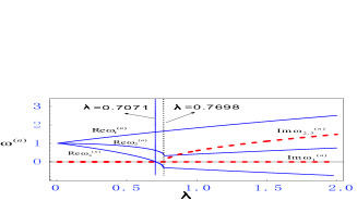
Figure 1: (Color online) The real part (thin solid lines) and imaginary part (thick dashed lines) of the eigenfrequencies vs the coupling parameter $\lambda$ in units of $\omega_{0}$ in the normal phase at the resonance case $\omega=\omega_{0}$.

Below, we focus only on the properties of eigen-frequencies in order to explore the existence of quantum criticality. Since the matrix $M^{(n)}$ is of $6\times 6$, general analytic results for the diagonalization of $\hat{\eta}M^{(n)}$ are difficult to obtain. Nevertheless, we can diagonalize it numerically to obtain the eigen-frequencies $\omega_{1,2,3}^{(n)}$ reduce . The related canonical transformation matrix $T^{(n)}$ can also be obtained numerically. Figure 1 shows the numerical results for the real and imaginary parts of $\omega_{1,2,3}^{(n)}$. For simplicity, we illustrate the resonant case $\omega=\omega_{0}$ $=$ $1$ here. Certainly, the non-resonance cases can also be studied numerically, with similar features being revealed. As seen from Fig. 1, when $\lambda>0.7698$, the imaginary parts of two eigen-frequencies are non-zero. This means that the corresponding eigen-frequencies are complex and thus the eigen state is unstable and physically impossible. But it is inappropriate to consider naively that $\lambda=0.7698$ as the critical point. Since the eigenvalue $\omega_{3}^{(n)}$ is negative in the range of $\lambda\in(0.7071,0.7698)$, a negative eigen-frequency of the boson-mode is not allowed physically either. Therefore, in the resonance case $\omega=\omega_{0}$ ($=1$), a real critical point is located at $\lambda_{c}^{(n)}=0.7071=\sqrt{2}/2$. In addition, for a general case, the critical point is found to be $\lambda_{c}^{(n)}=\sqrt{\omega\omega_{0}/2}$.

IV Super-radiant phase

In order to describe excitations in the parameter region above the critical point, we now incorporate the fact that both the field and the atomic collective excitations acquire macroscopic occupations, namely, the above approximation to neglect the number of excitations over $N$ is no longer valid emary . To this aspect, the introduced collective operators $B^{\dagger}$ and $C^{\dagger}$ in Eq. (2) should be expressed approximately as liusun

$$B^{\dagger} = b^{\dagger}\sqrt{1-\frac{b^{\dagger}b}{N}},\ \$$ (27)

$$C^{\dagger} = c^{\dagger}\sqrt{1-\frac{c^{\dagger}c}{N}},$$

in terms of  the Bose operators $b^{\dagger},b,c^{\dagger}$ and $c$. This transformation maps the original light-atoms system to a coupling three-mode bosonic system with the Hamiltonian

$$H^{(s)} = \omega_{0}(b^{\dagger}b+c^{\dagger}c)+\omega a^{\dagger}a+\lambda a^{\dagger}$$

$$\times\left(c^{\dagger}\sqrt{1-\frac{c^{\dagger}c}{N}}+\sqrt{1-\frac{b^{\dagger}b}{N}}b\right)+H.c..$$

For the present super-radiant phase, the bosonic modes may be displaced in the following way:

$$a^{\dagger} \rightarrow d^{\dagger}+\alpha^{\ast};\text{ }$$

$$b^{\dagger} \rightarrow e^{\dagger}-\beta^{\ast};\text{ }$$

$$c^{\dagger} \rightarrow f^{\dagger}-\gamma^{\ast},$$ (29)

where $\alpha$, $\beta$ and $\gamma$ are generally complex parameters in the order of $\emph{O}(\sqrt{N})$ emary to be determined later. This is equivalent to assume that all modes behave as the nonzero, macroscopic mean fields above $\lambda_{c}^{(n)}$.

Keeping the terms up to the order of $\emph{O}(N^{0})$, the Hamiltonian (IV) becomes

$$H^{(s)} = \left\{\lambda\sqrt{\frac{k_{\mathrm{f}}}{N}}\left[d^{\dagger}f^{\dagger}+\frac{(\alpha^{\ast}f^{\dagger}-\gamma^{\ast}d^{\dagger})}{2k_{\mathrm{f}}}(\gamma f^{\dagger}+\gamma^{\ast}f)\right]\right.$$ (30)

$$\left.+\lambda\sqrt{\frac{k_{\mathrm{e}}}{N}}\left[de^{\dagger}+\frac{(\alpha e^{\dagger}-\beta^{\ast}d)}{2k_{\mathrm{e}}}(\beta e^{\dagger}+\beta^{\ast}e)\right]+h.c.\right\}$$

$$+\omega d^{\dagger}d+\omega_{e}e^{\dagger}e+\omega_{f}f^{\dagger}f+\mathrm{c}_{\mathrm{0}}^{(s)},$$

where the constant term

$$\mathrm{c}_{\mathrm{0}}^{(s)} = \omega\left|\alpha\right|^{2}+\omega_{0}(\left|\beta\right|^{2}+\left|\gamma\right|^{2})$$ (31)

$$-\frac{2\lambda\alpha}{\sqrt{N}}(\beta^{\ast}\sqrt{k_{\mathrm{e}}}+\gamma\sqrt{k_{\mathrm{f}}})$$

will substantially contribute to the ground state energy at critical point; the renormalized frequencies

$$\omega_{e} = \omega_{0}+\lambda\alpha^{\ast}\beta/\sqrt{Nk_{\mathrm{e}}},$$

$$\omega_{f} = \omega_{0}+\lambda\alpha\gamma/\sqrt{Nk_{\mathrm{e}}},$$

with $k_{\mathrm{e}}=N-\left|\beta\right|^{2}$ and $k_{\mathrm{f}}=N-\left|\gamma\right|^{2}$. In the derivation of Eq. (30), the terms being linear in the bosonic operators are eliminated by choosing the appropriate displacements $\alpha$, $\beta$ and $\gamma$ in the following four cases:

$$\alpha^{(1,2,3,4)}=\frac{2\mathrm{e}^{i\phi}\lambda}{\omega}\sqrt{\frac{X_{+}X_{-}}{N}},$$ (35)

$$\left\{\begin{array}[]{l}\beta^{(j)}=\mathrm{e}^{i\phi}\sqrt{X_{\mp}},\ \ \ \text{(}j=1,3\text{)}\\ \gamma^{(j)}=\mathrm{e}^{-i\phi}\sqrt{X_{\mp}},\text{\ (}j=1,3\text{)},\end{array}\right.$$

or $$\left\{\begin{array}[]{l}\beta^{(j)}=\mathrm{e}^{i\phi}\sqrt{X_{\pm}},\ \ \ \text{(}j=2,4\text{)},\\ \gamma^{(j)}=\mathrm{e}^{-i\phi}\sqrt{X_{\mp}},\text{ (}j=2,4\text{)},\end{array}\right.$$ (38)

where $X_{\pm}=\frac{N}{2}(1\pm\frac{\omega\omega_{0}}{2\lambda^{2}})$, and $\phi$ is an arbitrary real number relating to the phases of displacements. In fact, we see from the form of $\alpha^{(j)}$ in Eq. (35) that only when

$$4\lambda^{4}-\omega^{2}\omega_{0}^{2}\geq 0,$$ (39)

$\alpha^{(j)}$ can be physically meaningful. Thus in the following discussions, it is required that

$$\lambda\geqslant\sqrt{\frac{\omega\omega_{0}}{2}}\ (=\lambda_{c}^{(n)}).$$

It is interesting to note that this threshed is just the critical point determined in the normal phase case.

Since $H^{(s)}(\phi)$ in Eq. (30) can be transferred to a $\phi$-independent Hamiltonian $H^{(s)}(\phi\equiv 0)$ through a unitary transformation

$$U(\phi)=e^{i\phi(d^{\dagger}d+e^{\dagger}e-f^{\dagger}f)},$$

we need only to look into the spectra of $H^{(s)}(0)$ in the four cases specified by Eq. (35), respectively. Because $H^{(s)}(0)$ is quadratic in each case, which is diagonalized by using the same method presented above as

$$H^{(j)} = \sum_{i=1}^{3}\omega_{i}^{(j)}\left(e_{i}^{(j)\dagger}e_{i}^{(j)}+\frac{1}{2}\right)$$ (40)

$$-\frac{1}{2}\mathrm{tr}\text{ }A^{(j)}+\mathrm{c}_{\mathrm{0}}^{(j)},\$$

for the four cases $j=1,...,4$. Here, the quasi-particle excitation is described by the boson vector operators

$$\mathrm{e}^{(j)} = (e_{1}^{(j)},e_{2}^{(j)},e_{3}^{(j)};e_{1}^{(j)\dagger},e_{2}^{(j)\dagger},e_{3}^{(j)\dagger})^{\mathrm{T}}$$

$$= T^{(j)}\left(d^{(j)},e^{(j)},f^{(j)};d^{(j)\dagger},e^{(j)\dagger},f^{(j)\dagger}\right)^{\mathrm{T}}$$

in the $j$-th phase, where

$$d^{(j)}=a-\left|\alpha^{(j)}\right|,\text{ }e^{(j)}=b+\left|\beta^{(j)}\right|,\text{ }f^{(j)}=c+\left|\gamma^{(j)}\right|$$

according to Eq. (29). $T^{(j)}$ is still the introduced unitary transformation to diagonalize

$$\hat{\eta}M^{(j)}=\left(\begin{array}[]{cc}A^{(j)}&B^{(j)}\\ -B^{(j)}&-A^{(j)}\end{array}\right),$$

where

$$A^{(1,3)} = \left(\begin{array}[]{ccc}\omega&A_{\mp}&C_{\mp}\\ A_{\mp}&\omega_{\mp}&0\\ C_{\mp}&0&\omega_{\mp}\end{array}\right),$$

$$B^{(1,3)} = \left(\begin{array}[]{ccc}0&C_{\mp}&A_{\mp}\\ C_{\mp}&B_{\mp}&0\\ A_{\mp}&0&B_{\mp}\end{array}\right),$$

$$A^{(2,4)} = \left(\begin{array}[]{ccc}\omega&A_{\pm}&C_{\mp}\\ A_{\pm}&\omega_{\pm}&0\\ C_{\mp}&0&\omega_{\mp}\end{array}\right),$$

$$B^{(2,4)} = \left(\begin{array}[]{ccc}0&C_{\pm}&A_{\mp}\\ C_{\pm}&B_{\pm}&0\\ A_{\mp}&0&B_{\mp}\end{array}\right),$$

with

$$\omega_{\pm} : =\omega_{0}+4\lambda^{2}X_{\pm}/N\omega,$$

$$B_{\pm} : =2\lambda^{2}X_{\pm}/N\omega,$$

$$A_{\pm} : =\lambda(X_{\mp}-X_{\pm}/2)/\sqrt{NX_{\mp}},$$

$$C_{\pm} : =-\lambda X_{\pm}/2\sqrt{NX_{\mp}}.$$

Clearly, $\omega_{i}^{(j)}$ ($i=1,2,3$) is the $i$-th eigenfrequency for the Hamiltonian $H^{(j)}$. Note that the canonical transformation matrix $T^{(j)}$ can be obtained numerically in the numerical diagonalization of $\hat{\eta}M^{(j)}$.

The numerical results of eigen-frequencies $\omega_{1,2,3}^{(j)}$ vs. the coupling parameter $\lambda$ are plotted in Fig. 2. The curves for both the real and imaginary parts of eigenfrequencies of $H^{(1)}$ in the resonant case are shown Fig. 2(a). It is found that the eigenfrequencies are physically reasonable when $\lambda>0.7071$ since the imaginary parts of all the eigenfrequencies are zero. This means a novel “quantum phase” emerges above the critical point

$$\lambda_{c}^{(1)}=\sqrt{\frac{\omega\omega_{0}}{2}}=0.7071.$$

It is seen from Fig. 2(a) that the eigenfrequency $\omega_{3}^{(1)}$ is always zero above $\lambda_{c}^{(1)}$, which implies that $H^{(1)}$ is reduced to have two independent boson modes. It is remarkable that the critical point is just the same one as that determined in the normal phase $\lambda_{c}^{(1)}=\lambda_{c}^{(n)}=\lambda_{c}$, demonstrating the consistency of our analysis.

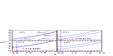
Figure 2: (Color online) The real part (solid lines) and imaginary part (dashed lines) of the eigenfrequencies vs the coupling parameter $\lambda$ in units of $\omega_{0}$ in the super-radiant phase at the resonance case $\omega=\omega_{0}$, where (a,b,c,d) correspond respectively to the cases (1,2,3,4) specified in the text.

In Fig. 2(b) [Fig. 2(d)], the numerical results for the real and imaginary parts of three eigenfrequencies of $H^{(2)}$ [$H^{(4)}$] in the resonant case. As seen from Fig. 2(b) [Fig. 2(d)], only when

$$\lambda>\lambda_{c}^{(2)}=0.8112\ (\lambda_{c}^{(4)}=0.8112),$$

another possible “quantum phase” may appear as the imaginary parts of all the eigenfrequencies are zero. While for $H^{(3)}$, as seen from Fig. 2(c), only when $\lambda>0.8457=\lambda_{c}^{(3)}$, the imaginary part of the all eigenfrequencies are zero, indicating a possible “quantum phase.”

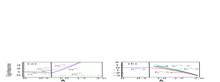
Figure 3: (Color online) (a) The eigenfrequencies for normal phase and the first super-radiant phase. (b) The ground state energy densities ($N=10^{6}$) for the normal phase and the super-radiant phases at the resonance case $\omega=\omega_{0}=1$.

In Fig. 3(a), we plot together the eigenfrequencies vs $\lambda$ for the normal phase and first super-radiant phase. The eigenfrequencies $\omega_{i}^{(n)}$ and $\omega_{i}^{(1)}$ (for $i=1,2,3$) are continuous at the critical point, respectively. Comparing with the results in the spatially independent Dicke model emary , our numerical studies show clearly that the excitation energy $\omega_{3}^{(n)}$ in the normal phase vanishes as $\left|\lambda-\lambda_{c}\right|^{zv}$ and the characteristic length scale $l_{3}=1/\sqrt{\omega_{3}^{(n)}}$ diverges as $\left|\lambda-\lambda_{c}\right|^{-v}$ at the quantum transition point $\lambda_{c}$, with the exponents given by $v=1/2$, $z=2$ on resonance; however, it is interesting to note that no critical exponents for $\omega_{3}^{(1)}$ in the super-radiant phase can be specified since $\omega_{3}^{(1)}\equiv 0$. Meanwhile, for the ground state, $\left\langle a^{\dagger}a\right\rangle_{G}/N=0$ below $\lambda_{c}$, while

$$\frac{\left\langle a^{\dagger}a\right\rangle_{G}}{N}=\left|\alpha^{(1)}\right|^{2}/N\propto(\lambda-\lambda_{c})$$

above $\lambda_{c}$, i.e., the field is macroscopically occupied. So $\alpha^{(1)}$ may be understood as a kind of order parameter of the super-radiant phase, whose critical exponent is $1/2$ above $\lambda_{c}$. In addition, Fig. 3(b) presents the ground-state energy densities as a function of coupling for all the possible phases. Clearly, the ground state energy densities of the first super-radiant phase is always the lowest one above $\lambda_{c}$, while the other three approach to it in the large $\lambda$ limit; moreover, it connects continuously with that of the normal phase but possesses a discontinuity in its second derivative at $\lambda_{c}$ through a detailed numerical analysis. From this viewpoint, together with the fact that the same critical point is determined from both sides of the normal phase and the first one, it is most likely that only the first super-radiant phase is a real physical one.

V Remarks and conclusions

Before concluding this paper, we wish to remark briefly on the origin of the occurred QPT in the present work. From Fig. 3(a), it is clear that the energy level of the first excited state of the system $(\omega_{3}^{(n)}+E_{0}^{(n)})$ touches the ground state energy level $E_{0}^{(n)}$ (or $E_{0}^{(1)}$) at the critical point. Obviously, it is this level touching that accounts for the emergence of the QPT and the corresponding quantum criticality in the present generalized Dicke model. It is also remarked that the $A^{2}$ terms (where $A$ is the vector potential) has been neglected here, as done in several previous works emary ; Reslen05 ; Vidal , while the absence of $A^{2}$ terms Rzazewski1 ; Rzazewski2 seems to be crucial for the observed quantum phase transition in the present model, namely, the presence of $A^{2}$ terms in the model Hamiltonian leads to vanishing of the criticality.

Although the effect of non-RWA terms may normally be negligibly small, the present work (also see Ref. emary ) illustrates that it plays a meaningful role when the atomic number $N$ is large, e.g., the criticality differs from that with the RWA. On the other hand, for actual atoms that may not be pure two-level ones, other atomic transitions may occur and spoil the present model before the non-RWA terms become important. Nevertheless, the present study is still theoretically interesting and valuable, particularly relevant to some atomic systems (or artificial and atomic-like ones) wherein the energy spacing of any other transitions is much larger than that of the considered two levels (or other transitions do not exist). For example, for a Dicke-like model consisting of many 1/2 spins coupled to single mode bosonic field (by electrical dipole coupling-like type), other transitions do not exist in the spin systems. Then the counter rotating terms play an important role the when the coupling parameter is close to the critical value.

In conclusion, based on a generalized Dicke model, we have investigated theoretically the quantum criticality of an extended atomic ensemble with a larger spacial dimension comparable to the optical wavelength of a quantized light field. A useful formalism is developed to study numerically eigenfrequencies of the system in different quantum phases. Comparing with the critical phenomenon around the critical point $\widetilde{\lambda}_{c}=\sqrt{\omega\omega_{0}}/2$ for atomic ensemble of small dimension emary , a rather different quantum criticality is revealed around the transition point ($\lambda_{c}=\sqrt{\omega\omega_{0}/2}=\sqrt{2}{\widetilde{\lambda}}_{c}$) from the normal phase to the super-radiant phase.

This work was supported by the NSFC with grant Nos. 90203018, 10474104, 60433050, 10447133, 10574133, & 10429401, the NFRP of China with funding Nos. 2001CB309310 and 2005CB724508, the RGC grant of Hong Kong (HKU7045/05P), and the URC fund of HKU.

References

• (1) S. Sachdev, Quantum Phase Transitions (Cambridge University Press, Cambridge, 1999).
• (2) C. Emary and T. Brandes, Phys. Rev. Lett. 90, 044101 (2003); C. Emary and T. Brandes, Phys. Rev. E 67, 066203 (2003).
• (3) J. Reslen, L. Quiroga, and N. F. Johnson, Europhys. Lett. 69, 8 (2005).
• (4) S. E. Harris, Physics Today 50, 36 (1997).
• (5) M. D. Lukin, Rev. Mod. Phys. 75, 457 (2003).
• (6) C. P. Sun, Y. Li, and X. F. Liu, Phys. Rev. Lett. 91, 147903 (2003).
• (7) K. Rzazewski, K. Wódkiewicz, and W. Zakowicz, Phys. Rev. Lett. 35, 432 (1975).
• (8) R. H. Dicke, Phys. Rev. 93, 99 (1954).
• (9) F. T. Hioe, Phys. Rev. A 8, 1440 (1973).
• (10) N. Lambert, C. Emary, and T. Brandes, Phys. Rev. Lett. 92, 073602 (2004).
• (11) J. Vidal and S. Dusuel, Europhys. Lett. 74, 817 (2006).
• (12) M. O. Scully, E. S. Fry, C. H. R. Ooi, and K. Wódkiewicz, Phys. Rev. Lett. 96, 010501 (2006).
• (13) C. Mewes and M. Fleischhauer, Phys. Rev. A  72, 022327 (2005).
• (14) Y. Li, L. Zheng, Yu-xi Liu, C. P. Sun, Phys. Rev. A 73, 043805 (2006).
• (15) Jean-Paul Blaizot, Quantum Theory of Finite Systems (Massachusetts Institute of Techology, 1986).
• (16) Actually, for the particlular $6\times 6$ dimensional matrix $\hat{\eta}M^{(n)}$ in this noraml phase, we have a simple method to diagonize it by reducing it into two $3\times 3$ dimensional sub-matrices (not presented here).
• (17) C. P. Sun, S. X. Yu, and Y. B. Gao, quant-ph/9809079; Yu-Xi Liu, C. P. Sun, S. X. Yu, and D. L. Zhou, Phys. Rev. A 63, 023802 (2001).
• (18) K. Rzazewski and K. Wódkiewicz, Phys. Rev. A 43, 593 (1991).
• (19) K. Rzazewski and K. Wódkiewicz, Phys. Rev. Lett. 96, 089301 (2006); V. Bužek, M. Orszag, and M. Roško, Phys. Rev. Lett. 96, 089302 (2006).