Chapter 1 Quantum Fractals. Geometricmodeling of quantum jumpswith conformal maps 

Arkadiusz Jadczyk

Abstract

Positive matrices in $SL(2,\mathbb{C})$ have a double physical interpretation; they can be either considered as “fuzzy projections” of a spin $1/2$ quantum system, or as Lorentz boosts. In the present paper, concentrating on this second interpretation, we follow the clues given by Pertti Lounesto and, using the classical Clifford algebraic methods, interpret them as conformal maps of the “heavenly sphere” $S^{2}.$ The fuzziness parameter of the first interpretation becomes the “boost velocity” in the second one. We discuss simple iterative function systems of such maps, and show that they lead to self–similar fractal patterns on $S^{2}.$ The final section of this paper is devoted to an informal discussion of the relations between these concepts and the problems in the foundations of quantum theory, where the interplay between different kinds of algebras and maps may enable us to describe not only the continuous evolution of wave functions, but also quantum jumps and “events” that accompany these jumps.
Keywords: Clifford algebras, conformal maps, iterated function systems, quantum jumps, quantum fractals.

1 Introduction

Let ${\bf B}^{3}=\{{\bf q}\in\mathbb{R}^{3}:\,{\bf q}^{2}\leq 1\}$ be the unit ball in $\mathbb{R}^{3}$ and let $S^{2}=\{{\bf p}\in\mathbb{R}^{3}:\,{\bf p}^{2}=1\}$ be the unit 2–sphere, that is the boundary of ${\bf B}^{3}.$ Every ${\bf q}\in\mathbb{R}^{3}$ determines a map $\phi_{{\bf q}}:S^{2}\rightarrow S^{2}$ through the formula:

$$\phi_{\bf q}({\bf p})\doteq\frac{(1-{\bf q}^{2}){\bf p}+2(1+{\bf q}\cdot{\bf p}){\bf q}}{1+{\bf q}^{2}+2{\bf q}\cdot{\bf p}}.$$ (1.1)

The formula (1.1) came naturally when discussing quantum jumps of a state of a spin $\frac{1}{2}$ particle [1]. During the 6-th ICCA Conference, Pertti Lounesto [2] conjectured that the maps $\phi_{\bf q},\,{\bf q}\in{\bf B}^{3},$ are conformal maps in that they preserve angles between vectors tangent to the sphere $S^{2},$ and he checked it numerically on randomly chosen tangent vectors using CLICAL [3]. Interesting patterns arise when the transformation $\phi_{{\bf q}}$ is iterated, that is applied many times, using different, symmetrically distributed ${\bf q}$’s. For instance, taking eight vectors ${\bf q}_{i},\,i=1,2,\ldots,,8,$ pointing from the origin to the eight corners of a cube inscribed in the unit sphere, all ${\bf q}_{i}$’s of length, say, $\|{\bf q}_{i}\|=0.74,$ we get the pattern shown in Fig. 1.

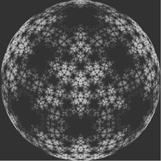
FIGURE 1: Quantum fractal based on eight vertices of a cube inscribed in the unit sphere $S^{2}$. 100,000,000 points obtained by a random choice of the initial point, followed by the application of randomly chosen conformal maps, with place–dependent probabilities $p_{i}$ given by the formula (3.11), from among eight maps defined by unit vectors ${\bf n}_{i}$–s situated at the eight vertices of a cube. View from above one of the vertices. Other closest three vertices are located at 60, 180 and 240 degrees. The dark areas are those that are (almost) never visited. The white areas are those that are frequently visited. The pattern shows distinct self–similarity - circles with circles. The details of algorithm are described in in Sec. 3

1.1 Iterated maps. Hausdorff distance, contractions, and attractor set.

Let $(X,d)$ be a complete metric space. In our examples $X$ will be a compact subset of the real plane $\mathbb{R}^{2}$ or a $2$–dimensional sphere $S^{2}=\{(x,y)\in\mathbb{R}^{2}:\,x^{2}+y^{2}=1\},$ which is also a complete metric space when endowed with the geodesic distance function $d(x,y)$ being the arc length along the great circle connecting $x$ and $y.$ Let ${\cal H}(X)$ be the set of all non–empty compact subsets of $X.$ A distance $h(Y,Z)$ (Hausdorff metric) between any two sets $Y,Z\subset X$ can be defined as follows. First define the distance between any point $x\in$ and any $Y\in{\cal H}(X)$ by

$$d(x,Y)=\{\min d(x,y):\,y\in Y\}.$$

Then, for any $X,Y\in{\cal H}(X)$ define the distance $d(Y,Z)$ from set $Y$ to set $Z$ by the formula

$$d(Y,Z)=\max\{d(y,Z):\ y\in Y\}.$$

The formula for $d(Y,Z)$ is not symmetric in $Y$ and $Z.$ Therefore one defines the Hausdorff distance $h(Y,Z)$ as the $\max$ of the two:

$$h(Y,Z)=\max(d(Y,Z),d(Z,Y)).$$

It can be shown that $h(Y,Z)$ is a metric on ${\cal H}(X).$ The definition of the Hausdorff distance is not very intuitive. There is an intuitive way to understand it: two sets are within Hausdorff distance $r$ from each other if and only if any point of one set is within distance $r$ from some point of the other set. From the fact that $X$ is also a complete metric space it can be then shown that ${\cal H}(X)$ endowed with the Hausdorff metric is a complete metric space, and therefore every Cauchy sequence $Y_{n}\in{\cal H}(X)$ has a limit in ${\cal H}(X).$ This property is crucial in proving the existence of attractor sets in studies of iterated function systems. A map $f:X\rightarrow X$ is a contraction  if there exists a constant $s,$ $0<s<1,$ called the contraction factor, such that $d(f(x),f(x^{\prime}))<s\cdot d(x,x^{\prime})$ for any two different points $x,x^{\prime}\in X.$ The so called Contraction Map Theorem states that in a complete metric space every contraction map $f$ has a unique fixed point $x_{0},$ i.e. such that $f(x_{0})=x_{0}.$ Moreover, for any initial point $x\in X$ the sequence $x_{n}=f^{(n)}(x),$ where $f^{(n)}=f\circ f\circ\ldots\circ f$ ($n$ times), converges to $x_{0}.$ Let now $f_{1},f_{2},\ldots f_{n}$ be contraction maps $f_{k}:X\rightarrow X,$ $k=1,2,\ldots n,$ with contraction factors $s_{k}.$. Then we can define a map $F$ acting on subsets $Y\subset X$ by the formula:

$$F(Y)=f_{1}(Y)\cup f_{2}(Y)\cup\ldots\cup f_{n}(Y)$$

where $Y\in{\cal H}(X)$ and $f_{k}(Y)$ is the image of the set $Y$ under the map $f.$ It can be shown that $F$ restricts to a map $F:{\cal H}(X)\rightarrow{\cal H}(X)$, and that this map is a contraction with the contraction factor $s=\max(s_{1},\ldots,s_{k}).$ It follows from the Contraction Mapping Theorem that $F$ has a unique fixed point, in that there is a unique compact subset $Y_{0}\subset X$ with the property that

$$Y_{0}=\bigcup_{k=1}^{n}f_{k}(Y_{0}).$$

This set $Y_{0}$ is called an attractor set  for the Iterated Function System consisting of the family $(f_{1},\ldots,f_{n}).$ Finding a numerical approximation to the attractor set needs lot of computation. Even when we start with a one–point set, its image under $F^{(k+1)}$ may have $n^{k}$ points. In cases like that moving to probabilistic algorithms may drastically reduce the need for computing resources. Quantum theory, that is probabilistic in nature, offers naturally examples of Iterated Function Systems with probabilities assigned to the maps $f_{i}.$ Such a system is called “IFS with probabilities” [4, Ch. 9.1]. The simplest example is provided by three affine maps with Sierpinski triangle as the attractor set.

1.2 The Sierpinski triangle.

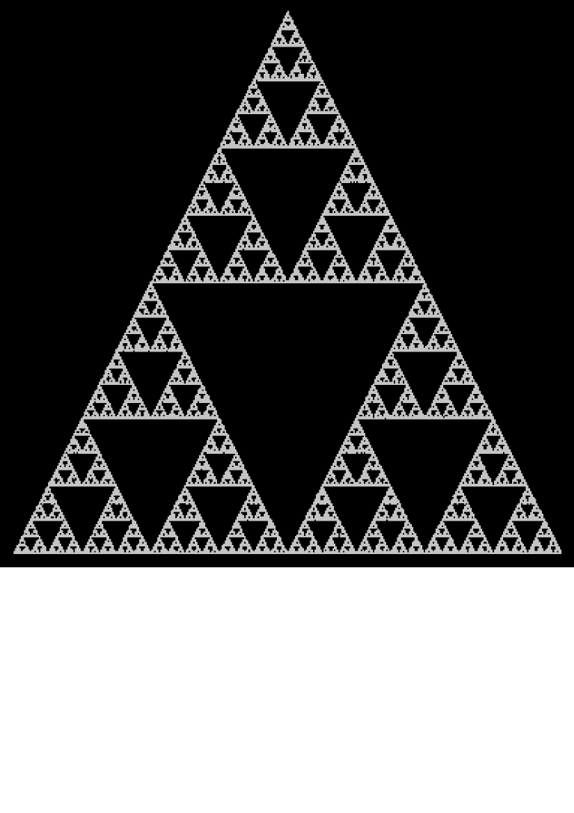
FIGURE 2: Sierpinski triangle. The attractor set of three non–commuting affine contractions.

An affine transformation of $\mathbb{R}^{2}$ is of the form $x\mapsto Ax+b,$ where $A$ is a $2\times 2$ matrix and $x,b\in\mathbb{R}^{2}.$ It is often convenient to represent such a transformation as a $3\times 3$ matrix

$${\tilde{A}}=\begin{pmatrix}A&a\cr 0&1\cr\end{pmatrix}$$

acting on $\mathbb{R}^{2}$ embedded in $\mathbb{R}^{3}$ as follows:

$$\begin{pmatrix}x\cr 1\cr\end{pmatrix}\mapsto\begin{pmatrix}A&a\cr 0&1\cr\end{pmatrix}\begin{pmatrix}x\cr 1\cr\end{pmatrix}=\begin{pmatrix}Ax+a\cr 1\cr\end{pmatrix}.$$

An affine transformation ${\tilde{A}}$ is a contraction  if for each $0\neq x\in\mathbb{R}^{2}$ we have that $\|Ax\|<\|x\|.$ Consider now three affine transformations ${\tilde{A}}[i],\quad i=1,2,3$ defined by

$${\tilde{A}}[i]=\begin{pmatrix}0.5&0&x[i]\cr 0&0.5&y[i]\cr 0&0&1\cr\end{pmatrix}$$

where $x[1]=y[1]=0,$ $x[2]=0.5,\,y[2]=0,$ $x[3]=0.25,\,y[3]=0.5.$ The transformations ${\tilde{A}}[i]$ do not commute. For instance ${\tilde{A}}[2]{\tilde{A}}[1]-{\tilde{A}}[1]{\tilde{A}}[2]$ is a translation by $0.25$ in the $x$ direction. They are also contractions, and they map the square $X=\{(x,y):\,0\leq x\leq 1,\,0\leq y\leq 1\},$ into itself (cf. [4][Ch. 3.7]). The probabilistic algorithm goes as follows: one starts with an arbitrary initial point $x_{0}$ and applies to it one of the three transformations $f_{i},$ selected randomly, each with the probability $p_{i}=1/3.$ One gets a new point $x_{1}.$ Then one of the transformations, again selected randomly, is applied to $x_{1}$ to produce $x_{2},$ etc. Each point is being plotted. The result of 100,000 transformations is presented in Fig. 2.

2 Möbius transformations of $S^{2}.$

2.1 Notation

We denote by $E_{(r,s)}$ the real vector space $\mathbb{R}^{n},$ $n=r+s,$ endowed with the quadratic form $q(x)$ of signature $(r,s).$ $E_{n}=E_{(n,0)}$ is the standard $n$–dimensional Euclidean space. The Clifford algebra of $E_{(r,s)}$ is denoted by $C(E_{(r,s)}),$ and the Clifford map $E_{(r,s)}\ni x\mapsto\phi(x)\in C(E_{(r,s)})$ satisfies $\phi(x)^{2}=q(x)I.$ $x$ and $\phi(x)$ are often identified. The principal automorphism of $C(E_{(r,s)})$ is denoted by $\pi$ and is determined by $\pi(x)=-(x),\,x\in E_{(r,s)},$ while the principal anti–automorphism $\tau$ is determined by $\tau(x)=x.$ Their composition $\nu$ is also denoted as $\nu(a)={\tilde{a}}$ and is the unique anti–automorphism satisfying ${\tilde{x}}=-x$ for all $x\in E_{(r,s)}.$ $\mathbb{C}(n)$ (resp $\mathbb{R}(n)$) will denote the algebra of complex (resp. real) matrices $n\times n.$
The Pauli spin matrices $\sigma_{0},\,\sigma_{1},\,\sigma_{2},\,\sigma_{3}$ are given by

$$\sigma_{0}\>=\>\left(\begin{array}[]{cc}1&0\\ 0&1\end{array}\right)\quad\sigma_{1}\>=\>\left(\begin{array}[]{cc}0&1\\ 1&0\end{array}\right)\quad\sigma_{2}\>=\>\left(\begin{array}[]{cc}0&-i\\ i&0\end{array}\right)\quad\sigma_{3}\>=\>\left(\begin{array}[]{cc}1&0\\ 0&-1\end{array}\right).$$

We have

$$X=\begin{pmatrix}x^{0}+x^{3}&x^{1}-ix^{2}\cr x^{1}+ix^{2}&x^{0}-x^{3}\cr\end{pmatrix},$$

thus $\det(X)=(x^{0})^{2}-{\bf x}^{2},$ and therefore an isomorphism of the Minkowski space $E_{(1,3)}$ with the $2\times 2$ hermitian matrices $X=X^{\star}.$ The inverse map $X\mapsto(x^{\mu})$ is given be $x^{\mu}=\frac{1}{2}\mbox{(}Tr)(\sigma_{m}uX).$ It is easy to verify that the Pauli matrices satisfy the following relations:

$$\sigma_{\mu}^{\star}=\sigma_{\mu},\qquad$$

$$\sigma_{k}\sigma_{l}=i\epsilon_{klm}\sigma_{m},$$

$$\frac{1}{2}\mbox{Tr}(\sigma_{\mu}\sigma_{\nu})=\delta_{\mu\nu},$$

$$\frac{1}{2}\mbox{Tr}(\sigma_{k}\sigma_{l}\sigma_{m})=i\epsilon_{klm},$$

$$\frac{1}{2}\mbox{Tr}(\sigma_{j}\sigma_{k}\sigma_{l}\sigma_{m})=\delta_{jk}\delta_{lm}+\delta_{jm}\delta_{kl}-\delta_{jl}\delta_{km},$$

where $\mu,\nu=0,1,2,3,$ and $j,k,l,m=1,2,3.$ The map $E_{3}\ni{\bf x}\mapsto\sigma({\bf x})=x^{1}\sigma_{1}+x^{2}\sigma_{2}+x^{3}\sigma_{3}$ is a Clifford map from $E_{3}$ to $\mathbb{C}(2),$ and $\mathbb{C}(2),$ as a real algebra, can be considered as the Clifford algebra of $E_{3}.$

2.2 $SL(2,\mathbb{C})$ as the group of Möbius transformations of $S^{2}.$

We will be interested in the particular case of $n=2,$ in which case the connected component of identity of the conformal group $Conf(\mathbb{R}^{2})$ is isomorphic to the ortochronous Lorentz group $SO_{+}(3,1).$ If we identify $S^{2}$ with the compactified complex plane $\mathbb{C}\cup{\infty},$ then conformal transformations form $Conf_{+}(\mathbb{R}^{2})$ can be conveniently realized by complex homographies $\mathbb{C}\ni z\mapsto\frac{az+b}{cz+d}$ ([5][Exercise 2.13.1]. For our purposes it will be more convenient to use the group $Spin(1,3)$ realized as $Sp(2,\mathbb{C})\approx SL(2,\mathbb{C}).$ We will start with describing the isomorphism of $Spin(1,3)$ to $SL(2,\mathbb{C})$ following the simple method given by Deheuvels in [7][Ch. X.6]

Every Hermitian $2\times 2$ matrix $X$ can be uniquely represented as

$$X=x^{\mu}\sigma_{\mu}$$

, with $x^{\mu}$ real, and where $\sigma_{\mu}$ are the Pauli matrices. For every $2\times 2$ matrix $A$ define $A^{\checkmark}\doteq CA^{t}C^{-1},$ where $A^{t}$ is the transposed matrix and

$$C=\begin{pmatrix}0&-1\cr 1&0\cr\end{pmatrix}.$$

Then $A\mapsto A^{\checkmark}$ is an anti–involution of the algebra $\mathbb{C}(2)$ and we have

$$A^{\checkmark}A=AA^{\checkmark}=\det(A)I$$

for all $A\in\mathbb{C}(2).$ In particular, $A\in SL(2,\mathbb{C})$ if and only if $A^{\checkmark}=A^{-1}.$ Notice that the anti–automorphisms $A\mapsto A^{\star}$ and $A\mapsto{\cal A}^{\checkmark}$ commute. Their composition denoted by $A\mapsto{\tilde{A}}=C{\bar{A}}C^{-1}$ is an involutive automorphism of the real algebra $\mathbb{C}(2),$ and it coincides with the automorphism $A\mapsto{\tilde{A}}$ if $\mathbb{C}(2)$ is considered as the Clifford algebra of $E_{3}$ with the Clifford map ${\bf x}\mapsto\sigma({\bf x}).$ Notice that for $A\in SL(2,\mathbb{C})$ we have ${\tilde{A}}=A^{\star}.$ It follows that the map $x\mapsto\phi(x)$ defined by

$$\phi(x)=\begin{pmatrix}0&X\cr X^{\checkmark}&0\end{pmatrix}$$

is a Clifford map from $E_{1,3}$ into the algebra $\mathbb{C}(4)$ od complex $4\times 4$ matrices. It is shown in [7][Théorème X.6] that $SL(2,\mathbb{C})$ can be identified then with the group $Spin(1,3)\subset\mathbb{C}(4)$ via the mapping

$$SL(2,\mathbb{C})\ni A\mapsto\begin{pmatrix}A&0\cr 0&\tilde{A}\cr\end{pmatrix}.$$

The action $Spin(1,3)$ on $E_{(1,3)}$ can be then easily computed in terms of $SL(2,\mathbb{C})$ matrices:

$$\begin{pmatrix}A&0\cr 0&{\tilde{A}}\end{pmatrix}\begin{pmatrix}0&X\cr X^{\checkmark}&0\end{pmatrix}\begin{pmatrix}A^{-1}&0\cr 0&{\tilde{A}}^{-1}\end{pmatrix}=\begin{pmatrix}0&X^{\prime}\cr{X^{\prime}}^{\checkmark}&0\end{pmatrix},$$

where $X^{\prime}=AX{\tilde{A}}^{-1}=AXA^{\star}.$ If $X=x^{\mu}\sigma_{\mu}$ then the map is accomplished by a Lorentz matrix ${\Lambda(A)^{\mu}}_{\nu}$ via

$$x^{\prime\mu}={\Lambda(A)^{\mu}}_{\nu}\,x^{\nu}.$$

Note: It is sometimes convenient to parametrize $GL(2,\mathbb{C})$ by complex Minkowski space coordinates $a^{\mu}\in\mathbb{C},$ via $A=a^{\mu}\sigma_{\mu}.$ It easily follows that $A\in SL(2,\mathbb{C})$ if and only if $a^{2}=(a^{0})^{2}-{\bf a}^{2}=1.$ Using the formulas of section 2.1 we can express the components of the Lorentz matrix ${\Lambda(A)^{\mu}}_{\nu}$ through the complex coordinates $a^{\mu}$ of $A$ as follows:

$${\Lambda^{0}}_{0}=|a^{0}|^{2}+|{\bf a}|^{2},$$

$${\Lambda^{0}}_{j}=2\Re({\bar{a}}^{0}a^{j})+i\epsilon_{jkl}a^{k}{\bar{a}}^{l}={\Lambda^{j}}_{0},$$

$${\Lambda^{j}}_{k}=(a\cdot{\bar{a}})\,\delta^{j}_{k}+2\Re(a^{j}{\bar{a}}^{k})+2\Im({\bar{a}}^{0}a^{l})\,\epsilon_{jkl}.$$

In order to describe explicitly the action of $SL(2,\mathbb{C})$ on $S^{2}$ it is convenient to embed $S^{2}$ in $E_{(1,3)}$ via $x^{0}=1$ section of the light–cone $x^{2}=0.$ That is we identify $S^{2}$ with the boundary of the unit ball $S^{2}=\{{\bf x}\in\mathbb{R}^{3}:{\bf x}^{2}=1\}=\{x=(x^{0},{\bf x})\in E_{(1,3)}:x^{0}=1,x^{2}=0\}.$ Given a unit vector ${\bf x}\in S^{2}\subset\mathbb{R}^{3},$ we associate with it the null vector $x=(1,{\bf x})\in E_{(1,3)},$ and therefore the matrix

$$X=\sigma_{0}+x^{i}\sigma_{i}=\begin{pmatrix}1+x^{3}&x^{3}-ix^{2}\\ x^{3}+ix^{2}&1-x^{3}\end{pmatrix}.$$

The matrix $X$ is positive and of determinant zero. The $SL(2,\mathbb{C})$ transformed matrix

$$X^{\prime}=AXA^{\star}$$ (2.2)

is also positive and of determinant zero. Therefore it represents another future oriented, null vector $x^{\prime},$ that corresponds to a unique vector ${\bf x}^{\prime}\in S^{2}$. In our application we will be interested in special conformal transformations of $S^{2},$ namely those generated by “pure boosts” of $SL(2,\mathbb{C}).$ By the polar decomposition theorem every matrix $A\in SL(2,\mathbb{C})$ can be uniquely decomposed into a product of a unitary and a positive matrix - both of determinant one. Unitary matrices represent three–dimensional rotations, while positive matrices represent special Lorentz transformations (boosts). The most general form of a positive $SL(2,\mathbb{C})$ matrix is

$$P({\bf n},\alpha)=c(I+\alpha\sigma({\bf n})),$$ (2.3)

where ${\bf n}\in S^{2}$ is a unit vector (the boost direction), and $0<\alpha=v/c<1$ is the “boost velocity”. Sometimes we will simply write $P({\bf q}),$ instead of $P({\bf n},\alpha),$ putting ${\bf q}=\alpha{\bf n}:$

$$P({\bf q})=(I+\sigma({\bf q})).$$ (2.4)

In the limit of $\alpha=1,$ which corresponds to “the velocity of light” $P$ degenerates into a projection operator, and we have $P({\bf x})=X,$ where $X$ represents the null vector $x=\{x^{\mu}\}=(1,{\bf x}),$ ${\bf x}\in S^{2}.$ Since $P({\bf q})=P({\bf q})^{\star},$ the action of the boosts $P({\bf q})$ on vectors ${\bf x}\in S^{2}$ given by the Eq. (2.2) can be found from the formula:

$$P({\bf q})P({\bf x})P({\bf q})=\lambda({\bf q},{\bf x})P({\bf x}^{\prime}).$$ (2.5)

A straightforward calculation gives

$$\lambda({\bf q},{\bf x})=\frac{1+{\bf q}^{2}+2\,{\bf q}\cdot{\bf x}}{4},$$ (2.6)

$${\bf x}^{\prime}=\frac{(1-{\bf q}^{2}){\bf x}+2(1+{\bf q}\cdot{\bf x}){\bf x}}{1+{\bf q}^{2}+2\,{\bf q}\cdot{\bf x}}.$$ (2.7)

Therefore we recover the formula (1.1) as coming from the special conformal transformation in the group $Spin(1,3).$ The crucial point in the above is to notice that $S^{2}$ is the one–point compactification of $E_{2}$ (the Riemann sphere), and that $E_{(3,1)}=E_{(2+1,0+1)},$ so that $Spin(1,3)=Spin(3,1)$ is the covering group of the conformal group for $E_{2}$ and $S^{2}.$

2.3 The geometrical meaning of the coefficient $\lambda({\bf q},{\bf x}).$

The numerical coefficient $\lambda({\bf q},{\bf x})$ in the formula (2.5) is not important for the transformation ${\bf x}\mapsto{\bf x}^{\prime}.$ Yet in the studies of iterated function systems not only the transformations themselves, but also the probabilities assigned to the transformations play an important role. For instance in Ref.[6, Chapter 6.3, p. 329] we find that for affine contractions it is advisable to choose the probabilities of maps to be proportional to the determinants of their linear parts. In our case the maps are Möbius transformations of $S^{2},$ and they are not contractions. In fact these maps contract some regions while expanding other regions. Is there a “natural” choice of probabilities, and can we use the place dependent factors $\lambda({\bf q},{\bf x})$ for determining the natural choice of probabilities? The answer is “yes”, though the exact formula is not at all evident. In [9] it is shown that by choosing $\lambda({\bf q},{\bf x})$’ as the relative probabilities of Möbius transformations (2.7), the iterated function system leads to a Markov semigroup that is linear. Moreover, denoting by $dS$ the rotation invariant area element of $S^{2},$ we find that this area changes as the result of the Möbius transformation (2.7) according to the formula:

$$\frac{dS^{\prime}}{dS}({\bf x})=\frac{(1-{\bf q}^{2})^{2}}{(1+{\bf q}^{2}+2{\bf q}\cdot{\bf x})^{2}}.$$ (2.8)

To visualize the mapping, let us assume that ${\bf q}=\alpha{\bf n},$ and that the vector ${\bf n}$ is along the $z$ axis: ${\bf n}=(0,0,1).$ Then all the region of the sphere above the critical value of $z=-\alpha$ is contracted into the region of the sphere above $z=\alpha,$ and the region of the sphere below $z=-\alpha$ is expanded into the region of the sphere below $z=\alpha.$ The relative probability $\lambda({\bf q},{\bf x})$ of choosing the Möbius map determined by ${\bf q}=\alpha{\bf n}$ is highest, $\lambda_{max}=(1+\alpha)^{2},$ for ${\bf x}$ parallel to ${\bf n}$ and has the minimum, $\lambda_{min}=(1-\alpha)^{2}$ for ${\bf x}$ antiparallel to ${\bf n}.$ At the critical value of $z=-\alpha,$ we have $\lambda=1-\alpha^{2},$ which is the geometrical mean of $\lambda_{max}$ and of $\lambda_{min}.$

3 Quantum Fractals

In order to implement an IFS with Möbius maps of the type that we have discussed, we need $N$ unit vectors ${\bf n}_{i},\,i=1,\ldots,N,$ and $N$ constants $\alpha_{i},$ $0<\alpha_{i}<1.$ Each vector ${\bf n}_{i}$ determines the direction, while each constant $\alpha_{i}$ determines the velocity of the Lorentz boost that implements the Möbius transformation $\phi_{{\bf q}_{i}}$ of $S^{2}:$

$$\phi_{{\bf q}_{i}}({\bf p})\doteq\frac{(1-{\bf q}^{2}){\bf p}+2(1+{\bf q}_{i}\cdot{\bf p}){\bf q}_{i}}{1+{\bf q}^{2}+2{\bf q}_{i}\cdot{\bf p}},$$ (3.9)

with ${\bf q}_{i}=\alpha_{i}{\bf n}_{i}.$. The probability $p_{i}({\bf x})$ of selecting the map $\phi_{i}=\phi_{{\bf q}_{i}}$ is then given by:

$$p_{i}({\bf x})=\frac{\lambda({\bf q}_{i},{\bf x})}{\sum_{j=1}^{N}\lambda({\bf q}_{j},{\bf x})}.$$ (3.10)

Inspecting the formula (2.6) we see that the denominator $\sum_{j=1}^{N}\lambda({\bf q}_{j},{\bf x})$ simplifies essentially if all $\alpha_{i}$ are the same: $\alpha_{i}=\alpha,\,i=1,\ldots,N,$ and the vectors ${\bf n}_{i}$ average to zero: $\sum_{i=1}^{N}{\bf n}_{i}=0.$ In this case the formula for probabilities $p_{i}({\bf x})$ simplifies to:

$$p_{i}({\bf x})=\frac{1+\alpha^{2}+2\alpha\,{\bf n}_{i}\cdot{\bf x}}{N(1+\alpha^{2})}.$$ (3.11)

3.1 Pseudocode for generation of Möbius IFS

In order to implement the IFS described above we first need to choose a set of unit vectors ${\bf n}_{i},$ and a value of the constant $\alpha.$ For instance, to create the picture, like that in Fig. 1, we have chosen $\alpha=0.71,$ and the vectors ${\bf n}_{i}$ as pointing to the eight vectors of the cube inscribed into the unit sphere, with one of the vertices at the north pole:
${\bf n}_{1}=(0,0,1),$ ${\bf n}_{2}=(2\sqrt{2}/3,0,1/3),$ ${\bf n}_{3}=(-2\sqrt{2/3},0,1/3),$
${\bf n}_{4}=(-\sqrt{2}/3,-\sqrt{2/3},1/3),$ ${\bf n}_{5}=(\sqrt{2}/3,\sqrt{2/3},-1/3),$
${\bf n}_{6}=(\sqrt{2}/3,-\sqrt{2/3},-1/3),$ ${\bf n}_{7}=(-2\sqrt{2}/3,0,-1/3),$ ${\bf n}_{8}=(0,0,-1).$ The following pseudocode describes now the generation of an IFS with Möbius transformations:

  (select initial ${\bf x}$)

  ${\bf x}\leftarrow{\bf x}_{0}$

  (choose $imax,$ for instance)

  $imax\leftarrow 10000000$

  $icount\leftarrow 0$

  while $icount<imax$ do

     $icount\leftarrow icount+1$

     (select one of the maps $\Phi_{i}$)

     (first initialize probability)

     $p\leftarrow 0$

     (initialize maps counter)

     $i\leftarrow 0$

     (choose a random number $0<r<1$)

     $r\leftarrow\mbox{random}(1)$

     repeat

        $i\leftarrow i+1$

        $p\leftarrow p+p_{i}({\bf x})$

     until $p>r$

     (the map $\phi_{i}$ is now selected, apply it)

     ${\bf x}\leftarrow\phi_{i}({\bf x})$

  end while

To create a graphic representation, such as in Fig. 1, we project the upper hemisphere onto the plane $(x,y),$ and divide the unit square of this plane into $r_{x}\times r_{y}$, for instance $600\times 600,$ rectangular cells, each cell being represented by one pixel on the screen. We associate a counter $c[ix][iy]$ with each of the cells $(ix,iy)$, initialize all counters to $0,$ and count points ${\bf x}=(x,y,z)$ that fall into the cell:

  $delta_{x}\leftarrow 2.0/r_{x};\,delta_{y}\leftarrow 2.0/r_{y}$

  $ix\leftarrow\mbox{round}((x-(-1.0))/delta_{x});\,iy\leftarrow\mbox{round}((y-(-1.0))/delta_{y})$

  (increase counter $c[i][j]$ by one:)

  $c[ix][iy]\leftarrow c[ix][iy]+1$

The next thing is to convert the values of the counters into grayscale tones. Here it is convenient to make grayscale proportional to $\log(c[i][j])$ rather than directly to $c[i][j],$ so as to be able to discern more details. In this case it is necessary to initialize the counters to the starting value of $1,$ rather than to $0.$ That is how Fig. 1 was created. Fig. 3, was created using a similar method, for six vertices of the regular octahedron, and using $\alpha=0.4,0.5,0.6,0.7,0.8$ and $0.9,$ but with the help of CLUCalc Visual Calculator, developed by Christian B.U. Perwass [10].

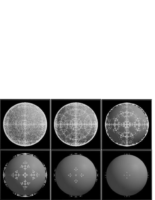
FIGURE 3: Quantum Fractal created with six vertices forming a regular octahedron, for $\alpha=0.4,0.5,\ldots,0.9.$

4 From Quantum Fractals to Clifford algebras and beyond

There are several deficiences of the standard quantum theory. For instance:

1. Need for external interpretation of the formalism

2. Need for an “observation”

3. Two kinds of evolution: deterministic one, formalized by the Schrödinger equation and “projection postulate” of not so clear status (what constitutes a measurement?)

4. Dubious role of time in Quantum Mechanics

5. Paradoxes, like that of Schrödinger cat

6. Impossibility of computer simulation of Reality (wave packet motion is not the only reality we want to explain)

It is striking that the concept of an “event” - which was of crucial importance in creating special and general theories of relativity finds no place in quantum formalism:

1. Barut [11], Bell [12, 13], Chew [14], Haag [15, 16], Shimony [17], Stapp [18, 19, 20, 21] and others stressed the inadequacy of the Standard Quantum Theory for describing real-time events

2. New technology enabled us to make continuous observations of individual quantum systems. These experiments give us time series of data - thus series of events and not only the expectation values (they may be ultimately computed)

3. What we observe are “events”. What we need to find and to explain are regularities in time series of events.

Einstein, Podolsky and Rosen [22] concluded that “the description of reality as given by a wave function is not complete.” John Stewart Bell, one of the most renowned theoretical physicists, [23] argued: “Either the wave function, as given by the Schrödinger equation, is not everything, or it is not right.(…) If, with Schrödinger, we reject extra variables, then we must allow that his equation is not always right. I do not know that he contemplated this conclusion, but it seems to me inescapable.” One year before his untimely and premature death, Bell wrote these insightful words in the paper that was his contribution to the Conference “62 Years of Uncertainty” held in Erice, Italy [13]:

The first charge against “measurement”, in the fundamental axioms of quantum mechanics, is that it anchors there the shifty split of the world into “system” and “apparatus”. A second charge is that the word comes loaded with meaning from everyday life, meaning which is entirely inappropriate in the quantum context. When it is said that something is “measured” it is difficult not to think of the result as referring to some preexisting property of the object in question. This is to disregard Bohr’s insistence that in quantum phenomena the apparatus as well as the system is essentially involved. If it were not so, how could we understand, for example, that “measurement” of a component of “angular momentum”…in an arbitrarily chosen direction…yields one of a discrete set of values? When one forgets the role of the apparatus, as the word “measurement” makes all too likely, one despairs of ordinary logic…. hence “quantum logic”. When one remembers the role of the apparatus, ordinary logic is just fine.

In other contexts, physicists have been able to take words from everyday language and use them as technical terms with no great harm done. Take for example the “strangeness”, “charm”, and “beauty” of elementary particle physics. No one is taken in by this “baby talk”…. as Bruno Touschek called it. Would that it were so with “measurement”. But in fact the word has had such a damaging effect on the discussion, that I think it should now be banned altogether in quantum mechanics.

Bogdan Mielnik [24], analyzing the “screen problem” - that is the event of a quantum particle hitting the screen - noticed that “The statistical interpretation of the quantum mechanical wave packet contains a gap”, which he specified as “The missing element of the statistical interpretation: for a normalized wave packet $\psi({\bf x},0)$ one ignores the probability of absorption on the surface of the waiting screen. The time coordinate of the event of absorption is not even statistically defined.” John Archibald Wheeler [25] wrote: “no elementary phenomenon is a phenomenon until it is a recorded phenomenon.” Eugene Wigner [26] (see also [27] for an overview of Wigner’s position) noticed that “there may be a fundamental distinction between microscopic and macroscopic systems, between the objects within quantum mechanics’ validity and the measuring objects that verify the statements of the theory.” Brian Josephson [28] suggested that ’the observer’ is a system that, while lying outside the descriptive capacities of quantum mechanics, creates observable phenomena such as wave function collapse through its probing activities. Better understanding of such processes may pave the way to new science.”

Motivated by these and other similar conclusions of many authors I decided to look for a “way out of the quantum trap”. While the real solution may need a radical departure from the present scheme of thinking about “Reality”, possible paths towards a better formalism than the standard one have been investigated by many authors, mainly along two lines. One is so called “Bohmian mechanics”, conceived originally by Louis de Broglie as “the theory of the double solution” [29], and then reformulated and developed by David Bohm [30] (see also [31, 32] for more recent reviews, and [33] for an interesting historical overview). The other is known as the GRW (Ghirardi–Rimini–Weber) or “spontaneous localization model” (see [34, 35]). In [36, 37] the GRW model has been generalized so as to apply not only to quantum mechanics, but also to quantum field theory (see also [38] for a recent comparison between the two approaches).

A further generalization of spontaneous localization theories has been described in [39], where a general formal structure of quantum theories that incorporate the concept of events has been formulated. This latter generalization enables us to define precisely the very concepts of “measurement” and “experiment”, along the paths suggested by John Bell, and to model simultaneous measurements of several non–commuting observables, in spite of the warnings of standard quantum mechanical textbooks claiming that such measurements contradict the very principles of quantum mechanics. As this subject is directly related to the main topic of this paper (the Möbius transformations $\phi_{\bf p},\,\phi_{\bf q}$ commute, only if ${\bf p}$ and ${\bf q}$ are parallel or antiparallel) , some introduction into the subject is given below.

The standard quantum theory, as formalized, for instance, by John von Neumann [40], was based on postulates, and on mathematical consequences derived from these postulates. The postulates were to a large extent arbitrary, and other systems of postulates have been proposed and discussed in the literature. Also the physical interpretation of the mathematical results is not unambiguous.

One of the most celebrated consequences of the quantum formalism is the so called Heisenberg’s uncertainty principle. Formally it states that in any quantum state the product $\Delta_{\psi}^{2}(x)\times\Delta_{\psi}^{2}(p_{x})$ of the mean square deviation from the mean values of the same components of the position and of the momentum variables are bounded from below by $\hbar^{2}/4.$ This formal result was, unfortunately, interpreted as an “impossibility of a simultaneous measurement of the position and momentum”, and, more generally, of any pair of complementary, non–commuting observables. I say “unfortunately”, because while it is true that non–commuting operators do not have, in general, a joint probability distribution, it has little to do with the possibility or impossibility of performing their simultaneous measurements; the main reason being that the concept of a “measurement” is not defined within the formal framework of the standard quantum theory.

To define the measurement an extension or a revision of the quantum theory is needed. The simplest extension is by using an algebraic formulation but, at the same time, abandoning the standard interpretation scheme. Let $\mathfrak{A}$ be an involutive algebra over $\mathbb{R}$ or $\mathbb{C},$ (for instance a $C^{*}$ or a von Neumann algebra), and let $\mathfrak{Z}$ be its center. When $\mathfrak{Z}$ is trivial (that is when it consists of scalars only), then $\mathfrak{A}$ is called a factor [41, Chapter V.1]. A general algebra can be, essentially uniquely, decomposed into a direct integral (or a direct sum) of factors [41, Theorem 8, p. 452]:

Theorem 1.

Let $\mathfrak{A}$ be a von Neumann algebra on a separable Hilbert space. Then $\mathfrak{A}$ is algebraically isomorphic to a direct integral of factors

$$\int_{X}\mathfrak{A}(t)\,d\mu(t).$$

Connes’ comment on this decomposition theorem is worth quoting:

“This theorem of von Neumann shows that the factors already contain what is original in all of the von Neumann algebras: they suffice to reconstruct every von Neumann algebra as a ‘generalized’ direct sum of factors.”

Although formally correct, the statement above is, at the same time, misleading. Every separable Hilbert space is a direct sum of one–dimensional spaces. But that does not mean that one–dimensional spaces contain what is original in all Hilbert spaces. For instance non–commutativity shows up only when the dimension of the Hilbert space is greater than one, and canonical commutation relations, so important in physics, can be realized only when the dimension of the Hilbert space is infinite; similarly with algebras.

In quantum theory it is usually assumed that the relevant algebras are factors. But, to include the “events”, to describe “measurements”, we need to go beyond that; we need to use more general algebras, with a non–trivial center. This step allows us, at the same time, to describe simultaneous “measurement” of several non–commuting observables. While there is no joint probability distribution, the process is well defined and leads to chaos and to fractal–like patterns, as seen, for instance, in Fig. 3 (see [42] for a comprehensive discussion of this issue).

The crucial issue here is illustrated by the double role of the maps $\phi_{q}$ (1.1). On on hand they are represented as belonging to the group $Spin(1,4)$ and therefore they are (inner) automorphisms of the Clifford algebra $C(E_{(1,4)}).$ On the other hand they are represented as linear, positivity preserving, transformations (see Eq. (2.2))of the complex algebra $\mathbb{C}(2)$ of $2\times 2$ complex matrices. The maps $X\mapsto X^{\prime}$ in Eq. (2.2) are not automorphisms, therefore they do not map central elements into central elements (even if the center is trivial in this particular case), yet they preserve positivity. It is positivity that is important in physical applications, because it relates to the positivity of probabilities.

Quantum mechanics has been, originally, formulated as a theory over the field of complex numbers. But there is no reason why it has to be so. The fields of real numbers and of quaternions lead to theories that are much like the standard quantum theory, except that the domains of application of these alternatives are not yet known.

The statistical interpretation of the standard quantum mechanics is based on the idea that the complex lines in a complex Hilbert space describe “pure states” of the system. But it does not have to be so. Other schemes are possible; any positive cone can serve as a statistical figure, and the probabilistic interpretation can result from dynamics (like in the simple IFS system discussed in this paper and in [39], see also [43] for a different approach to “Quantum Iterated Function Systems”), rather than be postulated. This opens the way towards generalization of the quantum mechanical framework and to a possible unification of quantum theory with relativity, a unification that has been sought for more than 70 years. Clifford algebras, and closely related CAR algebras (Canonical Anticommutation Relations), and their generalizations, provide one possible path. But there is also another path, going beyond algebras based on binary operations. First steps in this promising new direction have been taken by Frank D. Smith [45] and Yaakov Friedman [46] (see also [47] for the relevant mathematical background)

Acknowledgements: Thanks are due to the late Pertti Lounesto for pointing to me the path relating quantum jumps and conformal maps. I also thank Pierre Anglès for discussions and encouragement, and to QFG for a partial support of this work.

Arkadiusz Jadczyk

IMP

Chateau Saint Martin

Saint–Martin–Belcasse

82100 Castelsarrasin

France

E-mail: arkadiusz.jadczyk@cict.fr

Bibliography

- [1] A. Jadczyk, Topics in Quantum Dynamics, in Infinite Dimensional Geometry, Noncommutative Geometry, Operator Algebras and Fundamental Interactions, pp. 59–93, ed. R.Coquereaux et al., World Scientific, Singapore 1995, Preprint – http://arxiv.org/abs/hep-th/9406204
- [2] Pertti Lounesto, private communication
- [3] P. Lounesto, R. Mikkola, V. Vierros: CLICAL User Manual: Complex Number, Vector Space and Clifford Algebra Calculator for MS-DOS Personal Computers, Institute of Mathematics, Helsinki University of Technology, 1987
- [4] M. F. Barnsley, Fractals everywhere, Academic Press, San Diego 1988
- [5] Pierre Angles, Conformal Groups In Geometry And Spin Structures, Birkhauser, 2006
- [6] H. O. Peitgen, H. Jur̈gens, and D. Saupe, Chaos and Fractals: New Frontiers of Science, Springer-Verlag, New York: , 1992.
- [7] R. Deheuvels, Formes quadratiques et groupes classiques, PUF, 1981
- [8] A. Jadczyk, Piecewise Deterministic Quantum Dynamics and Quantum Fractals on the Poincare Disk, Rep. Math. Phys. 54 (2004), pp. 81–92
- [9] A. Jadczyk, Quantum fractals on –spheres, to appear.
- [10] Christian B. U. Perwass: CLUCalc - A Visual Calculator, v. 4.3.3, http://www.clucalc.info
- [11] A. O. Barut, Quantum Theory of Single Events: Localized De Broglie Wavelets, Schrödinger Waves, and Classical Trajectories, Found. Phys. 20 (1990), 1233–1240
- [12] J. S. Bell, Towards an exact quantum mechanics, in Themes in Contemporary Physics II. Essays in honor of Julian Schwinger’s 70th birthday, Deser, S. , and Finkelstein, R. J. Ed. , World Scientific, Singapore 1989
- [13] J. S. Bell, Against measurement, in Sixty-Two Years of Uncertainty. Historical, Philosophical and Physical Inquiries into the Foundations of Quantum Mechanics, Proceedings of a NATO Advanced Study Institute, August 5-15, Erice, Ed. Arthur I. Miller, NATO ASI Series B vol. 226 , Plenum Press, New York 1990
- [14] G. F. Chew, Gentle Quantum Events and the Source of Explicate Order, Zygon 20 (1985) 159–164
- [15] R. Haag, Fundamental Irreversibility and the Concept of Events, Commun. Math. Phys.132 (1990) 245–251
- [16] R. Haag, Events, histories, irreversibility, in Quantum Control and Measurement, Proc. ISQM Satellite Workshop, ARL Hitachi, August 28–29, 1992, Eds. H. Ezawa and Y. Murayama, North Holland, Amsterdam 1985
- [17] A. Shimony , Events and Processes in the Quantum World, in Quantum Concepts in Space and Time, Ed. R. Penrose and C. J. Isham, Clanderon Press, Oxford 1986
- [18] H. P. Stapp , Bell’s Theorem and World Process, Nuovo Cimento 29 (1975) 270–276
- [19] H. P. Stapp , Theory of Reality, Found. Phys. 7 (1977) 313–323
- [20] H. P. Stapp , Solution of the Infrared Problem, Phys. Rev. Lett. 50 (1983) 467–469
- [21] H. P. Stapp , Mind, Matter and Quantum Mechanics, Springer Verlag, Berlin 1993
- [22] A. Einstein, B. Podolsky, and N. Rosen, Can Quantum-Mechanical Description of Reality be Considered Complete?, Phys. Rev. 47 (1935), 777–780
- [23] J. S. Bell, Are there quantum jumps?, in Schrödinger, Centenary of a Polymath, Cambridge University Press (1987).
- [24] B. Mielnik , The Screen Problem , Found. Phys. 24 (1994) 1113–1129
- [25] J. A. Wheeler, Beyond the Black Hole, in Harry Woolf (ed.), Some Strangeness in the Proportion, A Centennial Symposium to Celebrate Achievements of Albert Einstein, Addison-Wesley, 1980
- [26] E. P. Wigner, Some Problems of our Natural Sciences, Int. J. Theoret. Phys. 25 (1986), 467–476
- [27] Olival Freire Jr, Orthodoxy and Heterodoxy in the Research on the Foundations of Quantum Physics: E. P. Wigner’s Case , Preprint – http://arxiv.org/abs/physics/0602028
- [28] B. D. Josephson, Beyond quantum theory: a realist psycho-biological interpretation of reality’ revisited, BioSystems, 64(2002)43–45
- [29] Louis de Broglie: Non-linear Wave Mechanics: A Causal Interpretation , Elsevier, Amsterdam, 1960.
- [30] D. Bohm, and B. J. Hiley,The Undivided Universe, Routledge, London, 1993
- [31] K. Berndl, M. Daumer, D. Dürr, S. Goldstein, N. Zanghi, A Survey on Bohmian Mechanics, Nuovo Cim. B110 (1995) 737-750
- [32] B. J. Hiley, R.E Callaghan, O. Maroney, Quantum trajectories, real, surreal or an approximation to a deeper process?, Preprint – http://arxiv.org/abs/quant-ph/0010020
- [33] Olival Freire Jr, Science and exile: David Bohm, the hot times of the Cold War, and his struggle for a new interpretation of quantum mechanics, Preprint – http://arxiv.org/abs/physics/0508184
- [34] G. C. Ghirardi, A. Rimini, T. Weber, Unified dynamics for microscopic and macroscopic systems, Phys. Rev. D 34, 470–491 (1986)
- [35] A. Bassi, G. C. Ghirardi, Dynamical Reduction Models, Phys. Rep. 379, (2003) 257–427, Preprint – http://arxiv.org/abs/quant-ph/0302164
- [36] Roderich Tumulka, On Spontaneous Wave Function Collapse and Quantum Field Theory, Preprint – http://arxiv.org/abs/quant-ph/0508230.
- [37] Roderich Tumulka, Collapse and Relativity, paper submitted to the proceedings of the conference “On the present status of quantum mechanics”, 7-9 September, 2005, Preprint – http://arxiv.org/abs/quant-ph/0602208
- [38] Valia Allori, Sheldon Goldstein, Roderich Tumulka, Nino Zanghi, On the Common Structure of Bohmian Mechanics and the Ghirardi-Rimini-Weber Theory, Preprint – http://arxiv.org/abs/quant-ph/0603027
- [39] A. Jadczyk, Some Comments on the Formal Structure of Spontaneous Localization Theories, paper submitted to the proceedings of the conference “On the present status of quantum mechanics”, 7-9 September, 2005, Preprint – http://arxiv.org/abs/quant-ph/0603046
- [40] J. von Neumann, Mathematical Foundations of Quantum Mechanics, Princeton Univ. Press, Princeton 1955
- [41] A. Connes, Noncommutative Geometry , Academic Press, San Diego 1994
- [42] A. Jadczyk, Measurement of Non-commuting Observables and Quantum Fractals on Complex Projective Spaces, Chinese Journal of Physics, 43, (2005) 301-327, Preprint – http://arxiv.org/abs/quant-ph/0311081
- [43] A. Lozinski, K. Zyczkowski and W. Slomczynski, Quantum Iterated Function Systems, Phys. Rev. E 68 (2003), 046110, Preprint – http://arxiv.org/abs/quant-ph/0210029
- [44] Erik Balslev and Andre Verbeure, States on Clifford algebras, Comm. Math. Phys. 7, (1968) 55 76
- [45] Frank D. (Tony) Smith, Jr., Hermitian Jordan Triple Systems, the Standard Model plus Gravity, and , Preprint – http://arxiv.org/abs/hep-th/9302030
- [46] Yaakov Friedman, Geometric tri-product of the spin domain and Clifford algebras, Preprint – http://arxiv.org/abs/math-ph/0510008
- [47] Ichiro Satake, Algebraic Structures of Symmetric Domains, Iwanami Shoten, Tokyo, and Princeton Univ. Press., Princeton, NJ, 1980