Vibration induced phase noise in Mach-Zehnder atom interferometers

Abstract

The high inertial sensitivity of atom interferometers has been used to build accelerometers and gyrometers but this sensitivity makes these interferometers very sensitive to the laboratory seismic noise. This seismic noise induces a phase noise which is large enough to reduce the fringe visibility in many cases. We develop here a model calculation of this phase noise in the case of Mach-Zehnder atom interferometers and we apply this model to our thermal lithium interferometer. We are thus able to explain the observed dependence of the fringe visibility with the diffraction order. The dynamical model developed in the present paper should be very useful to further reduce this phase noise in atom interferometers and this reduction should open the way to improved interferometers.

I Introduction

Atom interferometers have a large inertial sensitivity anandan77 ; clauser88 , which has been used to develop sensitive accelerometers kasevich91 ; kasevich92 ; cahn97 ; peters99 ; peters01 ; snadden98 ; mcguirk02 ; tino02 and gyrometers riehle91 ; lenef97 ; gustavson97 ; gustavson00 ; leduc04 ; landragin04 . However, because of this large sensitivity, a high mechanical stability of the experiment is required. This problem was recognized in 1991 by D. Pritchard and coworkers keith91 who were obliged to actively control the vibrations of the diffraction gratings of their Mach-Zehnder thermal atom interferometer. Since this work, various types of vibration control were developed: as an example, a very efficient control was developed by Chu and co-workers peters99 ; peters01 for the measurement of the local acceleration of gravity $g$. The problem obviously depends on the interferometer design and the present paper is devoted to an analysis of the vibration problem in three-grating Mach-Zehnder interferometers operated with thermal atoms.

In the present paper, we are going to evaluate the phase noise induced by mechanical vibrations in a Mach-Zehnder thermal atom interferometer. In our instrument, a very stiff rail holds the three diffraction gratings and this arrangement has strongly the effect of vibrations with respect to previous interferometers. We first analyze how the vibrations displace and distort the rail holding the gratings, by developing a simple model of the dynamics of this rail, using elasticity theory. This model will enable us to understand the contributions of various frequencies and to prove the importance of the vibration induced rotations of the rail. The predictions of this model will be tested in the case of our setup and the phase noise thus evaluated is in good agreement with the value deduced from fringe visibility measurements.

The paper is organized in the following way : part 2 recalls classic results concerning the inertial sensitivity of 3-grating Mach-Zehnder interferometers. Part 3 describes theoretically the motion and deformation of the rail holding the gratings and the resulting phase effect. Part 4 describes the rail of our interferometer and applies the present theory to this case. Part 5 discusses how to further reduce the vibration induced phase noise in this type of atom interferometers.

II Sensitivity of Mach-Zehnder atom interferometers to accelerations and rotations

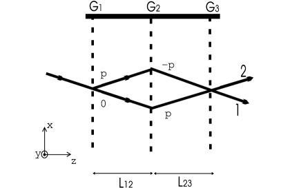
Figure 1: Schematic drawing of a three grating Mach-Zehnder atom interferometer, in the Bragg diffraction geometry. A collimated atomic beam is successively diffracted by three gratings $G_{1}$, $G_{2}$ and $G_{3}$. The diffraction orders are indicated on the various paths. Two exit beams, labelled $1$ and $2$, carry complementary signals. The $x$, $y$, $z$ axis are defined.

Atom interferometers are very sensitive to inertial effects anandan77 ; clauser88 . We consider a three-grating Mach-Zehnder atom interferometer represented schematically in figure 1 and we follow a tutorial argument presented by Schmiedmayer et al. in reference schmiedmayer97 . Each atomic beam is represented by a plane wave. When a plane wave $\Psi=\exp\left[i{\mathbf{k}}{\mathbf{r}}\right]$ is diffracted by a grating $G_{j}$, diffraction of order $p$ produces a plane wave:

$$\Psi_{d}({\mathbf{r}})=\alpha_{j}(p_{j})\exp\left[i{\mathbf{k}}\cdot{\mathbf{r}}+ip_{j}{\mathbf{k}}_{Gj}\cdot\left({\mathbf{r}}-{\mathbf{r}_{j}}\right)\right]$$ (1)

$\alpha_{j}(p_{j})$ is the diffraction amplitude; ${\mathbf{k}}_{Gj}$ is the grating wavevector, in the grating plane and perpendicular to its lines, with a modulus $k_{Gj}=2\pi/a$. The grating period $a$ is equal to $a=\lambda_{L}/2$ in the case of diffraction by a laser standing wave with a laser wavelength $\lambda_{L}$. This equation is exact for Bragg diffraction and a good approximation if ${\mathbf{k}}$ and ${\mathbf{k}}_{Gj}$ are almost perpendicular and $\left|{\mathbf{k}}_{Gj}\right|\ll\left|{\mathbf{k}}\right|$. Finally, ${\mathbf{r}_{j}}$ is a coordinate which measures the position of a reference point in grating $G_{j}$. Because of the presence of ${\mathbf{r}_{j}}$ in equation (1), the phase of the diffracted wave depends on the position of the grating in its plane and this dependence explains the inertial sensitivity of atom interferometers.

It is easy to calculate the waves exiting from the interferometer by the exit $1$ in figure 1, one wave $\Psi_{u}$ following the upper path with diffraction orders $p$, $-p$ and $0$ and the other wave $\Psi_{l}$ following the lower path with the diffraction orders $0$, $p$ and $-p$. These two waves produce an intensity proportional to $\left|\Psi_{u}+\Psi_{l}\right|^{2}$, which must be integrated over the detector surface. The condition ${\mathbf{k}}_{G1}+{\mathbf{k}}_{G3}=2{\mathbf{k}}_{G2}$ must be fulfilled to maximize the fringe visibility. We will assume that this condition is realized and that the grating wavevectors ${\mathbf{k}}_{Gi}$ are parallel to the $x$-axis. Then, the interferometer output signal $I$ measured at exit $1$ is given by:

$$I=I_{m}\left[1+{\mathcal{V}}\cos\Phi_{p}\right]\mbox{ with }\Phi_{p}=pk_{G}\left[2x_{2}-x_{1}-x_{3}\right]$$ (2)

where $I_{m}$ is the mean intensity, ${\mathcal{V}}$ is the fringe visibility defined by ${\mathcal{V}}=\left(I_{max}-I_{min}\right)/\left(I_{max}+I_{min}\right)$. When the gratings are moving, we must correct the grating-position dependent phase $\Phi$ in equation (2) by considering for each atomic wave packet the position of the grating $G_{j}$ at the time $t_{j}$ when the wavepacket goes through this grating:

$$\Phi_{p}=pk_{G}\left[2x_{2}(t_{2})-x_{1}(t_{1})-x_{3}(t_{3})\right]$$ (3)

If $=L_{12}/u$ is the atom time of flight $T=L_{12}/u$ from one grating to the next (with $L_{12}=L_{23}$ and $u$ being the atom velocity), $t_{j}$ are given by $t_{1}=t-T$ and $t_{3}=t+T$, where $t_{2}$ has been noted $t$. We can expand $\Phi$ in powers of $T$ by introducing the $x$-components of the velocity $v_{jx}(t)$ and acceleration $a_{jx}(t)$ of grating $G_{j}$ measured with reference to a Galilean frame. The phase $\Phi_{p}$ becomes:

$$\Phi_{p}=\Phi_{bending}+\Phi_{Sagnac}+\Phi_{acc.}$$ (4)

with $\Phi_{bending}=pk_{G}\delta(t)$ where the bending $\delta(t)=2x_{2}(t)-x_{1}(t)-x_{3}(t)$ is so called because it vanishes when the three gratings are aligned. The second term represents Sagnac effect because the velocity difference can be written $\left(v_{3x}-v_{1x}\right)=2\Omega_{y}L_{12}$, where $\Omega_{y}$ is the $y$-component of the angular velocity of the interferometer rail. Finally, the third term $\Phi_{acc.}=pk_{G}\left(a_{1x}+a_{3x}\right)T^{2}/2$ describes the sensitivity to linear acceleration anandan77 , slightly modified because the accelerations of the gratings $G_{1}$ and $G_{3}$ are different.

III Theoretical analysis of the rail dynamics

To calculate the phase $\Phi$, we are going to relate the positions $x_{j}(t_{j})$ of the three gratings to the mechanical properties of the rail holding the three gratings and to its coupling to the environment. A 1D theory of the rail is sufficient to describe the grating motions in the $x$ direction but we want to know the $x_{j}(t_{j})$ functions typically up to $10^{3}$ Hertz and the rail must be treated as an elastic object well before reaching $10^{3}$ Hz.

III.1 Equations of motion of the rail deduced from elasticity theory

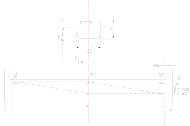
Figure 2: Drawings of our interferometer rail showing its shape and dimensions. Upper drawing: cross-section of the rail showing the two blocks and their dimensions ($200\times 50$ mm² for the lower block; $70\times 70$ mm² for the upper block). The planes of the two interferometers are indicated (A for the atom interferometer, B for the optical interferometer). Lower drawing: top view of the rail, with some details: positions of the mirrors $M_{i}$ for the three laser standing waves, position of the atomic beam and of the laser beams of the Mach-Zehnder optical interferometer.

The rail will be described as an elastic object of length $2L$, along the $z$ direction, which can bend only in the $x$ direction. The rail is made of a material of density $\rho$ and Young’s modulus $E$. The cross-section, with a shape independent of the $z$-coordinate, is characterized by its area $A=\int dxdy$ and by the moment $I_{y}=\int x^{2}dxdy$, the $x$-origin being taken on the neutral line. The neutral line is described by a function $X(z,t)$ which measures the position of this line with respect to a Galilean frame linked to the laboratory (in this paper, we forget that, because of Earth rotation, the laboratory is not a Galilean frame). Elasticity theory landauelasticity67 gives the equation relating the $t$- and $z$-derivatives of $X$:

$$\rho A\frac{\partial^{2}X}{\partial t^{2}}=-EI_{y}\frac{\partial^{4}X}{\partial z^{4}}$$ (5)

The rail is submitted to forces and torques exerted by its supports, which are related respectively to the third and second derivatives of $X$ with respect to $z$:

$$F_{x\epsilon}=-\epsilon EI_{y}\frac{\partial^{3}X}{\partial z^{3}}(z=\epsilon L)$$ (6)

$$M_{y\epsilon}=\epsilon EI_{y}\frac{\partial^{2}X}{\partial z^{2}}(z=\epsilon L)$$ (7)

$\epsilon=\pm$ labels the rail ends at $z=\epsilon L$. These torques and forces depend on the suspension of the rail. We assume that the torques vanish, which would be exact if the suspension was made in one point at each end and we consider that the forces are the sum of an elastic term proportional to the relative displacement and a damping term proportional to the relative velocity:

$$F_{x\epsilon}=-K_{\epsilon}\left[X(\epsilon L,t)-x_{\epsilon}(t)\right]-\mu_{\epsilon}\frac{\partial\left[X(\epsilon L,t)-x_{\epsilon}(t)\right]}{\partial t}$$ (8)

$x_{\epsilon}(t)$ is the coordinate of the support at $z=\epsilon L$. The spring constants $K_{\epsilon}$ and the damping coefficients $\mu_{\epsilon}$ may not be the same at the two ends of the rail. The damping terms have an effective character, because they represent all the damping effects.

III.2 Solutions of these equations

We introduce the Fourier transforms $X(z,\omega)$ and $x_{\epsilon}(\omega)$ of the functions $X(z,t)$ and $x_{\epsilon}(t)$. The general solution of equation (5) is:

$$X(z,\omega)=a\sin(\kappa z)+b\cos(\kappa z)+c\sinh(\kappa z)+d\cosh(\kappa z)$$ (9)

where $a$, $b$, $c$ and $d$ are the four $\omega$-dependent amplitudes of the spatial components of the function $X(z,\omega)$. $\omega$ and $\kappa$ are related by:

$$\rho A\omega^{2}=EI_{y}\kappa^{4}$$ (10)

Equations (6-8) relate $a,b,c,d$ to the source terms $x_{\epsilon}(\omega)$. Thanks to the assumption $M_{y\epsilon}=0$, $c$ and $d$ are related to $a$ and $b$:

$$c = a\sin(\kappa L)/\sinh(\kappa L)$$

$$d = b\cos(\kappa L)/\cosh(\kappa L)$$ (11)

and we get two equations relating $a$ and $b$ to $x_{\epsilon}(\omega)$:

$$\alpha_{\epsilon}a+\epsilon\beta_{\epsilon}b=\epsilon\gamma_{\epsilon}x_{\epsilon}(\omega)$$ (12)

where $\alpha_{\epsilon}$, $\beta_{\epsilon}$ and $\gamma_{\epsilon}$ are given in the appendix.

III.3 Analysis of the various regimes

To simplify, we assume that $K_{-}=K_{+}=K$ and $\mu_{-}=\mu_{+}=0$. $a(\omega)$ and $b(\omega)$ describe the transition from a low-frequency dynamics in which the rail moves almost like a solid to a high-frequency dynamics with a series of bending resonances. When the frequency is low enough, $\kappa L\ll 1$ because $\kappa\propto\sqrt{\omega}$ is also small and we expand the functions of $(\kappa L)$ up to third order (cubic terms in $\kappa L$ are needed to transmit a transverse force through the rail) and two resonances appear corresponding to pendular oscillations of the rail. The first resonance appears on the $b$ amplitude, when $R$ given by equation (24) verifies $R\approx 1$. This resonance corresponds to an in-phase oscillation of the two ends of the rail, with a frequency $\omega_{osc}=\sqrt{K/(\rho AL)}$. The second resonance, which appears on the $a$ amplitude when $R\approx 3$, describes a rotational oscillation of the rail around its center with a frequency $\omega_{rot}=\omega_{osc}\sqrt{3}$. If the two spring constants $K_{\epsilon}$ are different, these two resonances are mixed (each resonance appears on the $a$ and $b$ amplitudes) and their frequency difference increases.

For larger frequencies, $(\kappa L)$ is also larger and we cannot use power expansions of the functions of $(\kappa L)$. We then enter the range of bending resonances of the rail. If the forces $F_{x\epsilon}$ are weak enough, these resonances are almost those of the isolated rail which are obtained by writing that the equation system (12) has a nonvanishing solution when the applied forces vanish and the resonance condition is:

$$\cos(2\kappa L)\cosh(2\kappa L)=1$$ (13)

which defines a series of $\kappa_{n}$ values given approximately by:

$$\kappa_{n}L\approx(2n+3)\frac{\pi}{4}+\frac{(-1)^{n}}{\cosh\left[(2n+3)\pi/2\right]}$$ (14)

$n$ starts from $0$ (a more accurate value of $\kappa_{0}L$ is $\kappa_{0}L=2.365$) and $a=c=0$ when $n$ is even while $b=d=0$ when $n$ is odd. $\omega_{n}$ is deduced from $\kappa_{n}$, using equation (10). For a given length $L$, the wavevectors $\kappa_{n}$ are fixed, but the resonance frequencies $\omega_{n}$ increase with the stiffness of the rail measured by the quantity $EI_{y}/(\rho A)$. Finally, all the resonance frequencies $\omega_{n}$ are related to $\omega_{0}$, by $\omega_{n}=\omega_{0}(\kappa_{n}/\kappa_{0})^{2}$ with:

$$\omega_{0}=5.593\sqrt{EI_{y}/(\rho AL^{4})}$$ (15)

Introducing the period $T_{0}$ of the first bending resonance, $T_{0}=2\pi/\omega_{0}$, we may rewrite equation (10) in the form $(\kappa L)^{2}=0.890\times\omega T_{0}$. Finally, we have calculated the $Q$ factors of the various resonances (see appendix).

III.4 Effect of vibrations on the interferometer signal

The Fourier component $\Phi_{p}(\omega)$ of the phase $\Phi_{p}$ given by equation (3) can be expressed as a function of the amplitudes $a(\omega)$ and $b(\omega)$ given by solving the system (12). We assume that the gratings are on the neutral line, which means that $x_{i}(t_{i})=X(z_{i},t_{i})$ with $z_{1}=-L_{12}$ and $t_{1}=t-T$ for grating $G_{1}$, $z_{2}=0$ and $t_{2}=t$ for grating $G_{2}$ and $z_{3}=+L_{12}$ and $t_{3}=t+T$ for grating $G_{3}$. We get:

$$\frac{\Phi_{p}(\omega)}{2pk_{G}}= \left[b(\omega)\left(1-\cos(\kappa L_{12})+\left(1-\cosh(\kappa L_{12})\right)\frac{\cos(\kappa L)}{\cosh(\kappa L)}\right)\right.$$ (16)

$$+\left.ia(\omega)\left(\sin(\kappa L_{12})+\sinh(\kappa L_{12})\frac{\sin(\kappa L)}{\sinh(\kappa L)}\right)\sin\left(\omega T\right)\right.$$

$$+\left.b(\omega)\left(\cos(\kappa L_{12})+\cosh(\kappa L_{12})\frac{\cos(\kappa L)}{\cosh(\kappa L)}\right)\left(1-\cos(\omega T)\right)\right]$$

where the different lines correspond to the bending, the Sagnac and the acceleration terms in this order. We can simplify this equation by making an expansion in powers of $(\omega T)$ up to power $2$ and in powers of $\kappa L$ or $\kappa L_{12}$, up to fourth order:

$$\frac{\Phi_{p}(\omega)}{pk_{G}}\approx b\left(\frac{6(\kappa L)^{2}(\kappa L_{12})^{2}-(\kappa L_{12})^{4}}{6}\right)$$ (17)

$$+4ia(\kappa L_{12})\left(1-\frac{(\kappa L)^{2}}{6}\right)\left(\omega T\right)$$

$$2b(\omega T)^{2}$$

As in equation (4), we recognize the instantaneous bending of the rail (first line, independent of the time of flight $T$), the Sagnac term (second line, linear in $T$) and the acceleration term (third line, proportional to $T^{2}$). With the same approximations, $a$ and $b$ are given by equations (26,27). To further simplify the algebra, we replace the distance $L_{12}$ by $L$ ($L_{12}$ will usually be close to $L$) and we get:

$$\frac{\Phi_{p}(\omega)}{pk_{G}} \approx \left[x_{+}(\omega)-x_{-}(\omega)\right]\frac{3i(\omega T)}{\left(3-R\right)}$$ (18)

$$+ \left[x_{+}(\omega)+x_{-}(\omega)\right]\frac{0.330(\omega T_{0})^{2}+(\omega T)^{2}}{2(1-R)}$$

where $R$ is given by equation (24).

These three equations (16, 17, 18) are the main theoretical results of the present paper. Equation (18), which has a limited validity, because of numerous approximations, gives a very clear view of the various contributions. The first term, proportional to $\left[x_{+}(\omega)-x_{-}(\omega)\right]$ and to the time of flight $T$, describes the effect of the rotation of the rail excited by the out of phase motion of its two ends. This term, which is independent of the stiffness of the rail, is sensitive to the rail suspension through the $(3-R)$ denominator. The second term is the sum of the bending term, in $(\omega T_{0})^{2}$, and the acceleration term, in $(\omega T)^{2}$. Both terms are in $\omega^{2}$ and they also have the same sensitivity to the suspension of the rail, being sensitive to the first pendular resonance, when $R\approx 1$. The bending term is small if the rail is very stiff i.e. if the $T_{0}$ value is very small.

For larger frequencies ($\omega T\gtrsim 1$ or $\kappa L\gtrsim 1$), we must use numerical calculations of equation (16). We may note that, because $\omega\gg\omega_{osc},\omega_{rot}$, the $a$ and $b$ amplitudes will be small excepted near the bending resonances which appear either on the $b$ or $a$ amplitudes and do not contribute to the same terms of $\Phi_{p}(\omega)$.

IV Application of the present analysis to our interferometer

In this part, we are going to describe the rail of our interferometer and to characterize its vibrations.

IV.1 Information coming from previous experiments

When we built our interferometer in 1998, we knew that the vibration amplitudes encountered by D. Pritchard keith91 ; schmiedmayer97 and Siu Au Lee giltner95b ; giltner96 in their interferometers were large: for instance $\sqrt{\left<\delta(t)^{2}\right>}\approx 500$ nm after passive isolation by rubber pads in reference keith91 . In this experiment, each grating was supported on a flange of the vacuum pipe, which played the role of the rail. In the interferometer of Siu Au Lee and co-workers, a rail inspired by the three-rod design used for laser cavities was built giltner96 , but with a rod diameter close to $15$ mm, the rail was not very stiff. In both experiments, servo-loops were used to reduce $\delta(t)$ to observe interference signals.

IV.2 The rail of our interferometer

Rather than using servo-loops, we decided to achieve a very good grating stability by building a very stiff rail. We had to choose the material of the rail, its shape and its suspension, the main constraint being that the rail had to fit inside the DN250 vacuum pipe of our atom interferometer. The material must have a large value of $E/\rho$ ratio (Young’s modulus divided by density): we have chosen aluminium alloy rather than steel, both metals having almost the same $E/\rho$ ratio, because aluminium alloy is lighter and easier to machine. The shape of the rail must give the largest ratio $I_{y}/A$ with an open structure for vacuum requirements: we choose to make the rail as large as possible in the $x$ direction and rather thick to insure a good stiffness in the $y$ direction, because the $x$ and $y$ vibrations are not fully uncoupled. The rail, which is made of two blocks bolted together, is represented in figure 2. The lower block ($200$ mm wide and $50$ mm thick) provides the rigidity. Its length, $2L=1.4$ m, is slightly larger than twice the inter-grating distance $L_{12}=0.605$ m. The gratings, i.e. the mirrors of the laser standing waves, are fixed to the upper block, which has been almost completely cut in its middle to support the central grating. As a consequence, its contribution to the rigidity of the rail is probably very small and it will be neglected in the following calculation of the first bending resonance frequency $\omega_{0}/(2\pi)$: we use equation (15), with the full area $A\approx 1.49\times 10^{-2}$ m² but, for the moment $I_{y}$, we consider only the lower block contribution ($I_{y}\approx 3.3\times 10^{-5}$ m⁴). With $E=72.4\times 10^{9}$ N/m² and $\rho=2.79\times 10^{3}$ kg/m³, we calculate $\omega_{0}/2\pi\approx 437$ Hz.

When we built the suspension of the rail, the present analysis was not available and we made a very simple suspension: the rail is supported by three screws, two at one end and one at the other end, so that it can be finely aligned. Each screw is supported on a rubber block, model SC01 from Paulstra paulstra . These rubber blocks, made to support machine tools, are ring shaped with a vertical axis. The technical data sheet gives only a rough estimate of the force constant $K$ in the transverse direction, $K\approx 10^{6}$ N/m. As the total mass of our rail $\rho AL\approx 58$ kg, the pendular oscillations are expected to be at $\omega_{osc}/(2\pi)\approx 20$ Hz and $\omega_{rot}/2\pi\approx 35$ Hz. We have not taken into account the mixing of these resonances due to $K_{-}\neq K_{+}$, considering that the dominant uncertainty comes from the spring constant values.

IV.3 Test of the vibrations by optical interferometry

Following the works of the research groups of A. Zeilinger gruber89 ; rasel95 , D. Pritchard keith91 ; schmiedmayer97 and Siu Au Lee giltner95b ; giltner96 , the grating positions $x_{i}$ are conveniently measured by a 3-grating Mach-Zehnder optical interferometer. The phase $\Phi_{opt}$ of the signal of such an optical interferometer is also given by equation (4), with a negligible time delay $T$:

$$\Phi_{opt}=pk_{g,opt}\delta(t)$$ (19)

We have built such an optical interferometer miffre02 . The gratings from Paton Hawksley paton , with 200 lines/mm ($k_{g,opt}=3.14\times 10^{5}$ m^-1), are used in the first diffraction order with an helium-neon laser at a $633$ nm wavelength. The excitation of the rail by the environment gives very small signals, from which we deduce an upper limit of $\sqrt{\left<\delta(t)^{2}\right>}<3$ nm. This result is close to the noise (laser power noise and electronic noise) of the signal and the noise spectrum has not revealed any interesting feature.

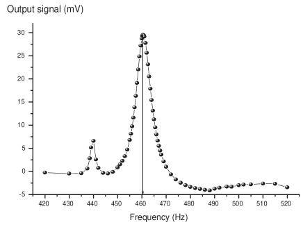
Figure 3: Response of the optical interferometer to an excitation of the rail oscillation: the modulation of the signal of the optical interferometer is plotted as a function of the frequency of the sine wave sent to the loudspeaker. We assign the main peak at $460.4$ Hz as due to the first bending resonance but the weaker peak near $440$ Hz is not assigned.

Hence, we have made a spectroscopy of the rail vibrations in the frequency domain by exciting its vibrations by a small loudspeaker fixed on the rail, close to its center, with the coil moving in the $x$-direction, so as to excite the $x$-bending of the rail. The loudspeaker was excited by a sine wave of constant amplitude and we have recorded with a phase-sensitive detection the modulation of the optical interferometer signal. Figure 3 presents the detected signal in the region of the first intense resonance centered at $\omega_{0}/(2\pi)=460.4$ Hz, with a rather large Q-factor, $Q\approx 60$. We have also observed a second resonance at $\omega_{1}/(2\pi)=1375$ Hz, with $Q\approx 65$, with a $30$ times weaker signal for the same voltage applied on the loudspeaker (the $n=1$ resonance appears on the $a$ amplitude and its detection by an optical interferometer, sensitive only to the $b$ amplitude, is due to small asymmetries) The first resonance frequency $460.4$ Hz is close to our estimate $437$ Hz and the observed frequency ratio $\omega_{1}/\omega_{0}\approx 2.99$ is also rather close to its theoretical value $2.76$, so that we can assign these two resonances as the $n=0$ and $n=1$ bending resonances of the rail, the discrepancies being due to oversimplifications of our model.

We have not observed any clear signature of the pendular oscillations on the optical interferometer signal, probably because the excitation and detection efficiencies are very low. The detection of these pendular oscillations will be done in a future experiment, using seismometers.

IV.4 Seismic noise spectrum: measurement and consequences for the atom interferometer phase noise

In the following calculation, we have not used our estimate of the first pendular resonance $\omega_{osc}/(2\pi)\approx 20$ Hz, because the predicted rms value of the bending $\sqrt{\left<\delta(t)^{2}\right>}$ was considerably larger than measured. We have used a larger value $\omega_{osc}/(2\pi)=40$ Hz, with $Q_{osc}=16$ and the measured $\omega_{0}$ value, $\omega_{0}/(2\pi)=460.4$ Hz. In our model with the simplifying assumptions $K_{-}=K_{+}=K$ and $\mu_{-}=\mu_{+}=\mu$, these three parameters suffice to describe our rail and its suspension.

In a first step, we calculate the $a$ and $b$ amplitudes as a function of one noise amplitude $x_{\pm}(\omega)$, the other one being taken equal to $0$. Figure 4 plots the ratios $\left|a(\omega)/x_{\epsilon}(\omega)\right|^{2}$ and $\left|b(\omega)/x_{\epsilon}(\omega)\right|^{2}$ as a function of the frequency $\nu=\omega/(2\pi)$: three resonances appear in the $1$-$10^{3}$ Hz range and, as expected, $a$ and $b$ decrease rapidly when $\omega>\omega_{osc},\omega_{rot}$, a decrease interrupted for $b$ by the first bending resonance.

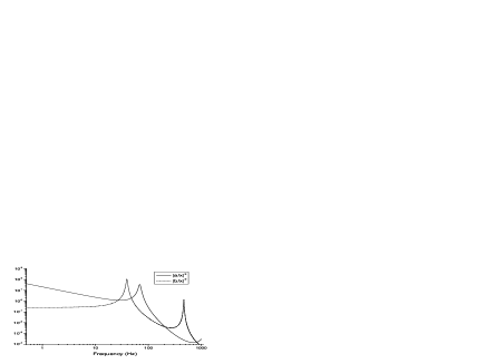
Figure 4: Logarithmic plot of the ratios $\left|a(\omega)/x_{\epsilon}(\omega)\right|^{2}$ and $\left|b(\omega)/x_{\epsilon}(\omega)\right|^{2}$ as a function of the frequency $\nu=\omega/(2\pi)$. Three resonances appear, which are the pendular oscillations, near $40$ and $69$ Hz, and the first bending resonance near $460$ Hz.

The seismic noise spectrum was recorded on our setup well before the operation of our interferometer. This spectrum presents several peaks appearing in the $8-60$ Hz range and most of these peaks do not appear on a spectrum taken on the floor, because they are due to resonances of the structure supporting the vacuum pipes. As the peak frequencies have probably changed because of modifications of the experiment since the recording, we have replaced the recorded curve by a smooth curve just larger than the measured spectrum. This noise spectrum $|x_{\epsilon}(\nu)|^{2}$ is plotted in figure 5. We have also extended the $\nu=0.5-100$ Hz frequency range to $\nu=0.5-10^{3}$ Hz, assuming the noise to be constant when $10^{2}<\nu<10^{3}$ Hz.

Figure 5 also plots the calculated phase noise spectrum $\left|\Phi(\nu)/p\right|^{2}$, using equation (16) and the Sagnac phase noise spectrum $\left|\Phi_{Sagnac}(\nu)/p\right|^{2}$ deduced from equation (16) by keeping only the term proportional to the $a$ amplitude: clearly, the Sagnac phase noise is dominant except near the in-phase pendular oscillation and the first bending resonance. The bending resonance is in a region where the excitation amplitude is very low, and, even after amplification by the resonance $Q$-factor, the contribution of the bending resonance to the total phase noise is fully negligible. In this calculation, we have assumed that the two excitation terms $x_{\epsilon}(\nu)$ have the same spectrum but no phase relation, so that the cross-term $\left|x_{+1}(\nu)x_{-1}(\nu)\right|$ can be neglected. This last assumption is bad for very low frequencies, for which we expect $x_{+1}(\nu)\approx x_{-1}(\nu)$ (as the associated correction cancells the Sagnac term, we have not extended the $\left|\Phi(\nu)/p\right|^{2}$ curves below $2$ Hz) but this assumption is good as soon as the frequency is larger than the lowest frequency of a resonance of the structure supporting the vacuum chambers (near $8$Hz).

Figure 5: Calculated phase noise spectra $\left|\Phi(\nu)/p\right|^{2}$ (full curve) and $\left|\Phi_{Sagnac}(\nu)/p\right|^{2}$ (dotted curve), both in rad${}^{2}/$Hz as a function of the frequency $\nu$ in Hz. The smoothed seismic noise spectrum $|x_{\epsilon}(\nu)|^{2}$ in m${}^{2}/$Hz used in the calculation is plotted (dashed curve) after multiplication by $10^{10}$.

By integrating the phase noise over the frequency from $2$ up to $10^{3}$ Hz, we get an estimate of the quadratic mean of the phase noise:

$$\left<\Phi^{2}\right>=0.16p^{2}\mbox{ rad}^{2}$$ (20)

This result is largely due to the Sagnac phase noise: the same integration on the Sagnac phase noise gives $\left<\Phi_{Sagnac}^{2}\right>=0.13p^{2}$ rad². We are going to test this calculation, using the measurements of fringe visibility as a function of the diffraction order $p$.

IV.5 Fringe visibility as a test of phase noise in atom interferometers

A phase noise $\Phi$ induces a strong reduction the fringe visibility ${\mathcal{V}}$:

$${\mathcal{V}}={\mathcal{V}}_{max}\exp\left[-\left<\Phi^{2}\right>/2\right]$$ (21)

assuming a Gaussian distribution of $\Phi$. When the phase noise is due to inertial effects (see equation (3)), $\Phi$ is proportional to the diffraction order $p$, $\Phi_{p}=p\Phi_{1}$. The fringe visibility ${\mathcal{V}}$ is a Gaussian function of the diffraction order $p$ delhuille02 :

$${\mathcal{V}}={\mathcal{V}}_{max}\exp\left[-\left<\Phi_{1}^{2}\right>p^{2}/2\right]$$ (22)

The atom interferometer of Siu Au Lee et al. giltner95b ; giltner96 and our interferometer miffre05 have been operated with the first three diffraction orders. The measured fringe visibility is plotted as a function of the diffraction order in figure 6 and Gaussian fits, following equation (22), represent very well the data. The quality of these fits suggests that phase noise of inertial origin is dominant and moreover that excellent visibility would be achieved in the absence of phase noise. With our data points, we deduce $\left<\Phi_{p}^{2}\right>=(0.286\pm 0.008)p^{2}$. Our estimate given by equation (20) is $56$% of this value and, considering the large uncertainty on several parameters (seismic noise, frequency and $Q$ factors of the pendular resonances), the agreement can be considered as good.

Figure 6: Fringe visibility as a function of the diffraction order $p$. Our measurements (round dots) are fitted by equation (22) with ${\mathcal{V}}_{max}=98\pm 1$ % and $\left<\Phi_{1}^{2}\right>=0.286\pm 0.008$. The data points of Giltner and Siu Au Lee (squares) are also fitted by equation (22) with ${\mathcal{V}}_{max}=85\pm 2$ % and $\left<\Phi_{1}^{2}\right>=0.650\pm 0.074$.

V How to further reduce the vibration phase noise in 3-grating Mach-Zehnder atom interferometers.

The phase noise induced by vibrations is very important and its reduction will considerably improve the operation of atom interferometers.

V.1 Servoloops on the grating positions

Pritchard and co-workers keith91 ; schmiedmayer97 as well as Giltner and Siu Au Lee giltner95b have used servo-loops to reduce the vibrational motion of the grating. The error signal was given by the optical Mach-Zehnder interferometer, which measures the instantaneous bending $\delta(t)=\left(2x_{2}(t)-x_{1}(t)-x_{3}(t)\right)$ and, as recalled above, in both experiments, the error signal before correction was large. In the experiment of Pritchard and co-workers, the correction was applied to the second grating. In the limit of a perfect correction, the bending term in equation (4) is cancelled and this correction does not modify the Sagnac and the acceleration terms. The fact that acting on the second grating has no inertial effects is a somewhat surprizing result, which can be explained by the symmetry of the Mach-Zehnder interferometer. In the experiment of Giltner and Siu Au Lee, the correction, which was applied to the third grating, cancels $\delta(t)$ but the Sagnac and acceleration terms are enhanced. In any case, the servo-loop can reduce the instantaneous bending $\delta(t)$ but it cannot reduce the Sagnac and acceleration terms. We think that a very stiff rail is a better solution for earth-based interferometers. For space based experiments, the phase noise spectra due to inertial vibration is different and the above solution may not be optimum, because of the large weight of the rail.

V.2 Possible improvements of the rail

The stiffness of our rail has reduced to a low level the bending and acceleration terms in the phase-noise of our interferometer. In our model, the rail stiffness is measured by only one parameter, the period $T_{0}$ of the lowest bending resonance, which scales with the rail length $L$ like $L^{2}$. Our $T_{0}$ value, $T_{0}=2.2\times 10^{-3}$ s, is still $3.8$ times larger than the time flight $T\approx 5.7\times 10^{-4}$ s in our experiment (lithium beam mean velocity $u=1065$ m/s; inter-grating distance $L_{12}=0.605$ m) and the bending term in equation (17) is $3$ times larger than the acceleration term. We can further reduce the bending term by reducing $T_{0}$, either by using an I-shaped rail to increase the $I_{y}/A$ ratio or by using a material with a larger $E/\rho$ ratio than aluminium alloy (for example, silicon carbide).

A defect of our rail is that it has no symmetry axis and the $x$ and $y$ bending modes are partly mixed. As the moment $I_{x}$ is considerably smaller than $I_{y}$, the bending resonances in the $y$-direction are at lower frequencies than in the $x$-direction. A better rail design should decouple almost completely the $x$ and $y$ vibrations.

V.3 Possible improvements of the suspension

The suspension of our rail is very primitive, with rather large spring constants and pendular resonances probably in the $\nu=20-100$ Hz range. A very different choice was made by J. P. Toennies and co-workers toennies03 : the rail was suspended by wires, the restoring forces being due to gravity. The pendular oscillation frequency is $\omega_{osc}=\sqrt{g/l}$, where $l$ is the wire length. For a typical $l$ value, $l=10$ cm, $\omega_{osc}/(2\pi)\approx 1.5$ Hz. In this experiment, a servo-loop was necessary to reduce the amplitudes of the pendular motions.

From the seismic noise spectrum of figure 5, it seems clear that the resonances of the suspension should not be in the $5$ to $30$ Hz range, where there is an excess noise. Our choice is not ideal and the choice of J. P. Toennies and co-workers toennies03 seems better, as the seismic noise in the $8-30$ Hz range can be largely reduced. Lower pendular resonance frequencies can be achieved by clever design (crossed wire pendulum, Roberts linkage) and a large know-how has been developed for the construction of gravitational wave detectors LIGO, VIRGO, GEO, TAMA, etc. Without aiming at a comparable level of performance, it should be possible to build a very efficient suspension.

V.4 Fringe visibility in atom interferometers

Since the first atom interferometry experiments in 1991, many different interferometers have been operated and numerous efforts have been done to improve these experiments. We are going to review the achieved fringe visibility, as this quantity is very sensitive to phase noise and other phase averaging effects (wavefront distorsions, $M$-dependent phase due to magnetic field gradient, etc). We have considered only Mach-Zehnder atom interferometers in which the atom paths are substantially different, excluding for instance atomic clocks. Our review is not complete, in particular because some publications do not give the fringe visibility. The measured values of the visibility are plotted in figure 7. Some low values are not only due to phase noise but also to other reasons: maximum visibility less than $100$ % in the case of Moir detection keith91 , parameters chosen to optimize the phase sensitivity lenef97 . Over a $15$-year period, impressive progress have been achieved and, hopefully, the same trend will continue in the future. The comparison with optical interferometry is encouraging as very high fringe visibility is routinely achieved in this domain.

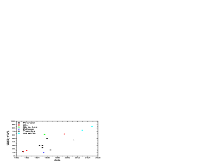
Figure 7: Fringe visibility ${\mathcal{V}}$ in three-grating atom interferometers as a function of the date of submission. These data points are taken from the following publications: Pritchard’s group keith91 ; ekstrom95 ; schmiedmayer95 ; roberts02 ; lenef97 ; chapman95 ; schmiedmayer97 ; Chu’s group kasevich91 ; kasevich92 ; peters99 ; Siu Au Lee’s group giltner95b ; giltner96 ; Zeilinger’s group rasel95 ; Toennies’s group meschede03 ; our works delhuille02a ; miffre05 .

VI Conclusion

The present paper has analyzed the phase noise induced in a Mach-Zehnder atom interferometer by mechanical vibrations. We have first recalled the inertial sensitivity of atom interferometers, following the presentation of Schmiedmayer et al. schmiedmayer97 . We have developed a simple $1$D model of the rail supporting the diffraction gratings. This model gives an unified description of the low-frequency dynamics, in which the rail behaves as a solid object, and the high frequency domain, in which rail bending cannot be neglected.

We have then described the rail of our interferometer. Our design has produced a very stiff rail and the bending of the rail due to vibrations appears to be almost negligible, while it was important in several previous experiments. In the low-frequency range, up to the frequency of the rotational resonance of the rail suspension, the out-of-phase vibrations of the two ends of the rail induce rotations of the rail, which are converted in phase noise by Sagnac effect: this is the dominant cause of inertial phase noise in our interferometer. A rapid decrease of the fringe visibility with the diffraction order has been observed by Siu Au Lee and co-workers giltner95b ; giltner96 and by our group miffre05 : the observed behavior is well explained as due to an inertial phase-noise and the deduced phase noise value is in good agreement with a value deduced from our model of the rail dynamics, using as an input the seismic noise measured on our setup.

In the last part, we have presented a general discussion of the vibration induced phase noise in 3-grating Mach-Zehnder interferometers. A reduction of this noise is absolutely necessary in order to operate atom interferometers either with higher diffraction orders or with slower atoms. In our experiment, a large reduction of this noise can be obtained by improving the suspension of the interferometer rail. Finally, we have reviewed the published values of the fringe visibility obtained with atom interferometers, thus illustrating the rapid progress since 1991.

VII Acknowledgements

We have received the support of CNRS MIPPU, of ANR and of Région Midi Pyrénées through a PACA-MIP network. We thank A. Souriau and J-M. Fels for measuring the seismic noise in our laboratory.

VIII Appendix: amplitudes of vibration of the rail and $Q$ factors of its resonances

Equations (6) and (8) relate the values of the $a$, $b$, $c$, $d$ amplitudes to $x_{\epsilon}(\omega)$. Using equation (III.2), we eliminate $c$ and $d$ to get the system of equations (12) with:

$$\alpha_{\epsilon} = \left[\cosh(\kappa L)\sin(\kappa L)-\sinh(\kappa L)\cos(\kappa L)\right]\cosh(\kappa L)$$

$$- 2(\kappa L)\cosh(\kappa L)\sinh(\kappa L)\sin(\kappa L)R_{\epsilon}^{-1}$$

$$\beta_{\epsilon} = \left[\cosh(\kappa L)\sin(\kappa L)+\sinh(\kappa L)\cos(\kappa L)\right]\sinh(\kappa L)$$

$$- 2(\kappa L)\cosh(\kappa L)\sinh(\kappa L)\cos(\kappa L)R_{\epsilon}^{-1}$$

$$\gamma_{\epsilon} = -(\kappa L)\cosh(\kappa L)\sinh(\kappa L)R_{\epsilon}^{-1}$$ (23)

with $R_{\epsilon}=\rho AL\omega^{2}/\left(K_{\epsilon}-i\mu_{\epsilon}\omega\right)$. From now on, $K_{-1}=K_{+1}=K$ and $\mu_{-1}=\mu_{+1}=\mu$. Then $\alpha$, $\beta$ and $\gamma$ are independent of $\epsilon$. $R$ can be expressed as a function of $\omega_{osc}=\sqrt{K/(\rho AL)}$ and $Q_{osc}=(\rho AL\omega_{osc})/\mu$:

$$R=\omega^{2}/\left[\omega_{osc}^{2}-i\frac{\omega_{osc}\omega}{Q_{osc}}\right]$$ (24)

We get $a$ and $b$:

$$a = \gamma(x_{+}-x_{-})/(2\alpha)$$

$$b = \gamma(x_{+}+x_{-})/(2\beta)$$ (25)

When $\kappa L\ll 1$, by expanding $\alpha$, $\beta$ and $\gamma$ in power of $\kappa L$ (up to the third order for $\alpha$), we get:

$$a=\frac{x_{+}-x_{-}}{4\kappa L}\times\frac{3}{3-R}$$ (26)

$$b=\frac{x_{+}+x_{-}}{4(1-R)}$$ (27)

$b$ exhibits a resonance when $R=1$ ($\omega=\omega_{osc}$) and $a$ when $R=3$ ($\omega=\omega_{osc}\sqrt{3}$). We have calculated the resonance $Q$ factors, in the weak damping limit. For an isolated resonance, the $Q$ factor is related by $Q=2\pi E_{tot}/\Delta E$ to the total energy $E_{tot}$ and the energy $\Delta E$ dissipated during one vibration period. We get:

$$Q_{osc}=\rho AL\omega_{osc}/\mu$$ (28)

$$Q_{rot}=\rho AL\omega_{rot}/(3\mu)$$ (29)

$$Q_{n}=\rho AL\omega_{n}g(\kappa_{n}L)/(8\mu)$$ (30)

where the function $g(\kappa_{n}L)$ depends on the parity of $n$:

$$g(\kappa_{n}L) = \left[1+\frac{\sin(2\kappa_{n}L)}{2\kappa_{n}L}\right]\left[\frac{1}{\cos^{2}(\kappa_{n}L)}+\frac{1}{\cosh^{2}(\kappa_{n}L)}\right]\mbox{ for even }n$$ (31)

$$= \left[1-\frac{\sin(2\kappa_{n}L)}{2\kappa_{n}L}\right]\left[\frac{1}{\sin^{2}(\kappa_{n}L)}+\frac{1}{\sinh^{2}(\kappa_{n}L)}\right]\mbox{ for odd }n$$

From the measured $Q$-factor of the first bending resonance ($n=0$), we get $\mu\approx 560$ kg.s^-1.

References

- (1) J. Anandan, Phys. Rev. D 15, 1448 (1977)
- (2) J. F. Clauser, Physica B 151, 262 (1988)
- (3) M. Kasevich and S. Chu, Phys. Rev. Lett. 67, 181 (1991)
- (4) M. Kasevich and S. Chu, Appl. Phys. B 54, 321 (1992)
- (5) S. B. Cahn, A. Kumarakrishnan, U. Shim, T. Sleator, P. R. Berman and B. Dubetsky, Phys. Rev. Lett. 79, 784 (1997)
- (6) A. Peters, K. Y. Chung and S. Chu, Nature 400, 849 (1999)
- (7) A. Peters, K. Y. Chung and S. Chu, Metrologia 38, 25 (2001)
- (8) M. J. Snadden, J. M. McGuirk, P. Bouyer, K. G. Haritos and M. A. Kasevich , Phys. Rev. Lett. 81, 971 (1998)
- (9) J. M. McGuirk, G. T. Foster, J. B. Fixler, M. J. Snadden, and M. A. Kasevich, Phys. Rev. A 65, 033608 (2002)
- (10) G. M. Tino, Nucl. Phys. B 113, 289 (2002)
- (11) F. Riehle, Th. Kisters, A. Witte, J. Helmcke and Ch. J. Bord , Phys. Rev. Lett. 67, 177 (1991)
- (12) A. Lenef, T. D. Hammond, E. T. Smith, M. S. Chapman, R. A. Rubenstein, and D. E. Pritchard, Phys. Rev. Lett. 78, 760 (1997)
- (13) T. L. Gustavson, P. Bouyer and M. A. Kasevich, Phys. Rev. Lett. 78, 2046 (1997)
- (14) T. L. Gustavson, A. Landragin and M. A. Kasevich, Class. quantum Grav. 17, 2385 (2000)
- (15) F. Leduc, D. Holleville, J. Fils, A. Clairon, N. Dimarcq, A. Landragin, P. Bouyer and Ch. J. Bordé, Proceedings of 16th ICOLS, P. Hannaford et al. editors, World Scientific (2004)
- (16) A. Landragin et al., Proceedings of ICATPP-7, World Scientific (2002)
- (17) D. W. Keith, C. R. Ekstrom, Q. A. Turchette and D. E. Pritchard, Phys. Rev. Lett. 66, 2693 (1991)
- (18) J. Schmiedmayer, M. S. Chapman, C. R.Ekstrom, T. D. Hammond, D. A. Kokorowski, A. Lenef, R.A. Rubinstein, E. T. Smith and D. E. Pritchard, in Atom interferometry edited by P. R. Berman (Academic Press 1997), p 1
- (19) Q. Turchette, D. Pritchard and D. Keith, J. Opt. Soc. Am. B 9, 1601 (1992)
- (20) C. Champenois, M. Büchner and J. Vigué, Eur. Phys. J. D 5, 363 (1999)
- (21) L. Landau and E. Lifchitz, Theory of Elasticity, Pergamon Press, Oxford (1986)
- (22) Paulstra company, website http://www.paulstra-vibrachoc.com
- (23) M. Gruber, K. Eder and A. Zeilinger, Phys. Lett. A 140, 363 (1989)
- (24) E. M. Rasel, M. K. Oberthaler, H. Batelaan, J. Schmiedmayer and A. Zeilinger, Phys. Rev. Lett., 75, 2633 (1995)
- (25) D.M. Giltner, R. W. McGowan and Siu Au Lee, Phys. Rev. Lett., 75, 2638 (1995)
- (26) D. M. Giltner, Ph. D. thesis, Colorado State University, Fort Collins (1996)
- (27) A. Miffre, R. Delhuille, B. Viaris de Lesegno, M. Büchner, C. Rizzo and J. Vigué, Eur. J. Phys. 23, 623 (2002)
- (28) Paton Hawksley Education Ltd, UK, website: http://www.patonhawksley.co.uk/
- (29) J. P. Toennies, private communication (2003)
- (30) R. Delhuille, A. Miffre, B. Viaris de Lesegno, M. Büchner, C. Rizzo, G. Trńec and J. Vigué, Acta Physica Polonica 33, 2157 (2002)
- (31) A. Miffre, M. Jacquey, M. Büchner, G. Trénec and J. Vigué, Eur. Phys. J. D 33, 99 (2005)
- (32) C. R. Ekstrom, J. Schmiedmayer, M. S. Chapman, T. D. Hammond and D. E. Pritchard, Phys. Rev. A 51, 3883 (1995)
- (33) J. Schmiedmayer, M. S. Chapman, C. R. Ekstrom, T. D. Hammond, S. Wehinger and D. E. Pritchard, Phys. Rev. Lett. 74, 1043 (1995)
- (34) T. D. Roberts, A. D. Cronin, D. A. Kokorowski1, and D. E. Pritchard, Phys. Rev. Lett. 89, 200406 (2002))
- (35) M. S. Chapman, C. R. Ekstrom, T. D. Hammond, R. A. Rubenstein, J. Schmiedmayer, S. Wehinger, and D. E. Pritchard, Phys. Rev. Lett. 74, 4783 (1995)
- (36) work of J. P. Toennies and R. Brühl quoted in D. Meschede, Gerthsen Physik, 22, 709 (2003)
- (37) R. Delhuille, C. Champenois, M. Büchner, L. Jozefowski, C. Rizzo, G. Trénec and J. Vigué, Appl. Phys. B 74, 489 (2002)