Entanglement dynamics of qubits in a common environment

Abstract

We use the quantum jump approach to study the entanglement dynamics of a quantum register, which is composed of two or three dipole-dipole coupled two-level atoms, interacting with a common environment. Our investigation of entanglement dynamics reflects that the environment has dual actions on the entanglement of the qubits in the model. While the environment destroys the entanglement induced by the coherent dipole-dipole interactions, it can produce stable entanglement between the qubits prepared initially in a separable state. The analysis shows that it is the entangled decoherence-free states contained as components in the initial state that contribute to the stable entanglement. Our study indicates how the environmental noise produces the entanglement and exposes the interplay of environmental noise and coherent interactions of qubits on the entanglement.

and and

1 Introduction

Entanglement is a remarkable feature of quantum mechanics and plays a fundamental role in quantum computation and quantum information processing. Due to its fundamental importance for quantum information processing, it has attracted much attention in recent years [1]. The entanglement can be produced either by direct interactions between qubits [2], or by indirect interactions between the qubits through a third party [3]. However, both of the above processes are constrained to the closed system where the influence of the environment is neglected. In real situations, a quantum system can never be isolated and will inevitably interact with its environment. A severe effect of this unwanted interaction is decoherence which generally leads to the degradation of quantum coherence and entanglement. Up to now, decoherence remains to be the main obstacle to the practical implement of quantum information processing. Recently, the influences of the environment on the entanglement have been investigated extensively [4, 5, 6, 7, 8, 9, 10, 11]. It was found that in certain cases the environment can act as a third party and be constructive to the production of the entanglement, in contrast to its destructive role in the ordinary situations. That is to say, depending on different coupling mechanisms between the environment and quantum system in different models, the environment has dual nature influenced on the entanglement between the qubits.

In the present work, we will show that this dual influences can be present simultaneously even in one model under certain given coupling mechanism between the environment and system. For this purpose, we model a quantum register by two or three two-level atoms with dipole-dipole interactions. We study its entanglement dynamics (i.e. the time evolution of entanglement quantity [8, 12, 13, 14, 15]) under the influence of a common environment. The direct interactions between the qubits have not been considered in the previous works [4, 5, 6, 7, 8]. The environment used here is treated as a reservoir of quantum harmonic oscillators with infinite degrees of freedom [16], in contrast to the single-mode model used by Kim et al. [4]. By introducing a collective mode consisting of all the qubit modes and eliminating the enormous irrelevant degrees of freedom of the environment, a quantum master equation of the atomic system can be obtained under the Born-Markovian approximation. We use the quantum jump approach [17] to study the time evolution behaviors of bi- and tri-partite entanglement defined by the concurrence [18] and the negativity [19], respectively. Originally, the quantum jump approach [17] was proposed to study the transition dynamics of a single atom system (for a review, see, e.g. [20]) and has been used to obtain the operator solution of the master equation [20, 21]. The merit of using quantum jump approach is that it supplies a simple way to obtain the solution of master equation in the multipartite system with a very large Hilbert space. The dynamical behavior of the bi- and tri-partite entanglement shows clearly that the environment has dual nature influenced on the entanglement in the system studied. On the one hand, it destroys entanglement induced by the dipole-dipole interactions, which shows the decoherence nature of the environment. On the other hand, it induces stable entanglement in an incoherent way, which shows the third party role of the environment. Different from the previous works [4, 5, 6, 7, 8], the dual nature of the environment is shown simultaneously in the same system in our situation. The stable entanglement induced by the environment is very different from the simple oscillation behavior of entanglement with time obtained by Kim et al. [4], where the memory effect of the single-mode environment was considered. Here we point out that the environment in our model as a reservoir has no memory effect under the Markovian approximation. The environment induces entanglement in an incoherent way since with infinite degrees of freedom it introduces an irreversibility to the dynamics of the qubit system.

The paper is organized as follows. In Section II we introduce the model and the quantum jump approach. In Section III we study the entanglement dynamics of a two-qubit system. The entanglement dynamics of a three-qubit system is discussed in Section IV. Finally, Section V is devoted to a brief summary.

2 Model and quantum jump approach

We consider a quantum register composed of $N$ (=2 and 3 in the following discussions) identical two-level atoms coupled by dipole-dipole interactions. These atoms are assumed to be located very near, so that they feel a common environment and interact collectively with the environment. The environment is modeled by an electromagnetic field with infinite degrees of freedom which is assumed at vacuum state. If the collective interaction between atoms and the common environment is very weak and the characteristic time of correlation function of the environment is very short compared with the time scale of system evolution, then Born and Markovian approximations are valid. By the standard method of quantum optics [16], the master equation of the reduced density matrix of the system can be derived

$$\frac{d\rho\left(t\right)}{dt}=-i[H_{I},\rho\left(t\right)]+\frac{\gamma}{2}(2J_{-}\rho\left(t\right)J_{+}-J_{+}J_{-}\rho\left(t\right)-\rho\left(t\right)J_{+}J_{-}),$$ (1)

where $\gamma$ is the decay constant of the collective mode represented by

$$J_{\pm}=\sum_{i=1}^{N}\sigma_{\pm}^{i}\text{, \ \ \ \ \ }J_{z}=\sum_{i=1}^{N}\frac{\sigma_{z}^{i}}{2},$$

and

$$H_{I}=\sum_{i>j}^{N}(g_{ij}\sigma_{+}^{i}\sigma_{-}^{j}+h.c.)$$

describes the dipole-dipole interactions of the qubits. The first term on the right-hand side of Eq. (1) generates a coherent unitary evolution of the density matrix, while the second term represents the decoherence effect of the environment on the system and generates an incoherent dynamics of system. It should be noted that in general case the strengths of dipole-dipole interactions are dependent on the positions of the atoms. But in our model, the separation of the atoms are very small compared to the wavelengths of the most relevant field modes, so that the fields induce a global dipole-dipole interactions(in the long wavelength limit), i.e. $g_{i,j}=g$. Thus the interaction Hamiltonian becomes

$$H_{I}=g\left(J_{+}J_{-}-J_{z}-\frac{N}{2}\right).$$

By using individual mode representation Eq. (1) can be rewritten as

$$\frac{d\rho\left(t\right)}{dt}=-i[H_{I},\rho\left(t\right)]+\frac{\gamma}{2}\sum_{i,j=1}^{N}(2\sigma_{-}^{i}\rho\left(t\right)\sigma_{+}^{j}-\sigma_{+}^{j}\sigma_{-}^{i}\rho\left(t\right)-\rho\left(t\right)\sigma_{+}^{j}\sigma_{-}^{i}).$$ (2)

It should be pointed out that the terms with $i=j$ in the sum on the right-hand side of Eq. (2) denote the individual dissipation of each atom due to the environment, while the $i\neq j$ terms describe the couplings between the atoms indirectly induced by the common environment.

The master equation (1) has been used for many years to study the superradiance effect involving the interaction of collective atomic systems with the radiation field [22, 23]. The collective interaction between the atoms and the radiative field can induce two typical atomic states with an enhanced (the superradiant state) and a reduced (the subradiant state) spontaneous decay rate. When the atoms are confined in a very small region, the subradiant state is completely decoupled from the environment, and therefore can be regarded as a decoherence-free state. A related experiment on the superradiant spontaneous emission of two trapped ions has been reported [24].

The common feature of the quantum master equations is the existence of the sandwich terms, where the reduced density matrix of the system is in between some quantum excitation and de-excitation operators. In general, the master equation is converted into c-number equation [16, 23]. In this paper, we use the quantum jump approach to obtain the exact operator solution of the master equation (1). As mentioned above, the quantum-jump approach was proposed to describe single experimental realizations of simple quantum systems (i.e. two- and three-level atoms) [17] and has been extensively used in quantum optics [20]. By using the quantum jump approach, it is straightforward to obtain the exact operator solution of the master equation. The advantage of using this method is that one does not need to deal with each element of the reduced density matrix individually, the time-dependent solution of the reduced density matrix can be obtained directly from the formal solution under the actions of operators.

By the quantum jump approach the reduced density matrix $\rho\left(t\right)$ can be written as a sum of the conditional density matrices $\rho^{(n)}(t)(n=1,2,\cdots)$ as follows

$$\rho\left(t\right)=\sum_{n}\rho^{(n)}\left(t\right)=\sum_{n}Tr_{F}\{\mathbb{Q}_{n}\rho_{tot}\left(t\right)\},$$

where $\rho_{tot}$ is the total density matrix of the system and the quantized environment, $Tr_{F}\{\cdot\}$ is the partial trace over the modes of the environment, and $\mathbb{Q}_{n}$ is the projection operator on the state of the quantized environment field that contains $n$ photons. The $\rho^{(n)}\left(t\right)$ denotes the reduced density matrix of the system with $n$ photons detected in the environment. The time evolution equation of $\rho^{(n)}\left(t\right)$ can be derived readily,

$$\frac{d\rho^{(n)}\left(t\right)}{dt}=-i(H_{eff}\rho^{(n)}\left(t\right)-\rho^{(n)}\left(t\right)H_{eff}^{\dagger})+\gamma J_{-}\rho^{(n-1)}\left(t\right)J_{+}(1-\delta_{n0}),$$ (3)

where $H_{eff}=H_{I}-\frac{i\gamma}{2}J_{+}J_{-}$. Eq. (3) reflects that the time evolution of the reduced density matrix consists of smooth evolutions which are interrupted by instantaneous quantum jumps. It is clear to see that the hierarchy of the conditional density matrices $\rho^{(n)}(t)$ is terminated by instantaneous quantum jumps automatically. Due to the dissipative effect of the environment, the effective Hamiltonian $H_{eff}$ governed the smooth evolution is a non-Hermitian operator. It is straightforward to write down the formal operator solution of Eq. (3)

$$\rho^{(0)}(t) = e^{-iH_{eff}t}\rho(0)e^{iH_{eff}^{\dagger}t},$$

$$\rho^{(n)}(t) = \gamma\int_{0}^{t}dt^{\prime}e^{-iH_{eff}(t-t^{\prime})}J_{-}\rho^{(n-1)}(t^{\prime})J_{+}e^{iH_{eff}^{\dagger}(t-t^{\prime})},$$ (4)

where $\rho(0)$ is the initial state. Thus, the total reduced density matrix of the system can be obtained by the summation over all the conditional density operators $\rho^{(n)}\left(t\right)$. In the following we explicitly consider the two-qubit and three-qubit systems.

3 Entanglement dynamics in a two-qubit system

To simplify the following calculations, we use the collective state representation [23]. The representation space is spanned by the common eigenstates of the complete set of commuting operators $\{J^{2},J_{z}\}$ for two-qubit system. This collective state representation can also be obtained by the angular momentum additive rules and the Clebsch-Gordan coefficients from the product state representation of the individual ones [25]. The two-qubit basis denoted by $|j,m\rangle$ includes the spin singlet and triplet

$$|0,0\rangle=\frac{1}{\sqrt{2}}(|+-\rangle-|-+\rangle)$$

$$|1,1\rangle=|++\rangle,$$

$$|1,0\rangle=\frac{1}{\sqrt{2}}(|+-\rangle+|-+\rangle),$$

$$|1,-1\rangle=|--\rangle,$$ (5)

where $|\pm\rangle$ are the eigenstates of $\sigma_{z}$ with elgenvalus $\pm 1$, respectively. The $J_{\pm}$ act on the collective basis by

$$J_{\pm}|j,m\rangle=\sqrt{j(j+1)-m(m\pm 1)}|j,m\pm 1\rangle.$$

When a total system is composed of two subsystems described by a two-dimensional Hilbert state, the general measure of entanglement between these two subsystems is the entanglement of formation [26]. This quantity can be analytically calculated as a function of the concurrence $C$ [18], which can also be taken as a measure of the entanglement. The concurrence is defined as

$$C=\max(0,\lambda_{1}-\lambda_{2}-\lambda_{3}-\lambda_{4}),$$ (6)

where $\lambda_{i}(i=1,\cdots,4)$ are eigenvalues of the matrix $[\rho^{1/2}(\sigma_{y}\otimes\sigma_{y})\rho^{\ast}(\sigma_{y}\otimes\sigma_{y})\rho^{1/2}]^{1/2}$. Here $\rho^{\ast}$ is the complex conjugation of $\rho$. The concurrence varies from $C=0$ for a disentangled state to $C=1$ for a maximally entangled state. We shall use the concurrence to quantify the degree of entanglement in the two-qubit system.

Figure 1: The time evolution of the concurrence $C(t)$. The pair of atoms is initially prepared in the state $\rho(0)=|+-\rangle\langle+-|$ for $g=1.0$ (solid line), $0.2$ (dashed line), and $0$ (dotted line) and $\gamma=0.1$.

In the following numerical investigations, our guide line is to explore the following topics of entanglement dynamics:

(1) Two kinds of entanglement generation mechanisms and their different roles played: direct coherent generation due to the atomic dipole-dipole interaction and indirect incoherent generation due to the common environment coupling to the qubits. From Eq. (1) we can see that the atomic dipole-dipole interactions in $H_{I}$ produce a dynamical coherence which oscillates in time, and the common environment induces an effective interaction which produces the entanglement in steady states. Besides, the common environment also produces a dissipative term which makes all the eigen states of the operator of the master equation decay and finally die out except the steady states with zero eigen values [8]. Thus in the dissipative dynamics, the dynamical coherence as a transit phenomenon will be destroyed finally by the dissipation, only the environment induced coherence and entanglement in the decoherence-free steady states survive. In the following numerical study, the two kinds of entanglement generation show clearly in the figures.

(2) How does the environment produce an entangled steady state from a separable initial state? This issue is closely related to the generation of an entanglement source and is thus very significant.

(3) How does the entanglement measure evolve and change in time from an initial entangled state under the influence of the common environment? This issue is related to the decoherence of a multi-qubit system and is thus practically helpful in the understanding of the decoherence dynamics.

(4) As the decoherence-free subspace has more than one dimensions, the steady state will be a probabilistic mixture of the decoherence-free states. How does one choose a proper initial state to get a desired steady state?

In order to show explicitly the entanglement dynamics of the two-qubit system, we take the initial state $\rho(0)=|+-\rangle\langle+-|$ as our first example. Expanding this state in the collective basis of Eqs. (5) and substituting it into Eqs. (4), we can obtain analytically the solution of the master equation (1) after some calculations

$$\rho(t) = \frac{e^{-2\gamma t}}{2}|1,0\rangle\langle 1,0|+\frac{1-e^{-2\gamma t}}{2}|1,-1\rangle\langle 1,-1|$$ (7)

$$+\frac{1}{2}|0,0\rangle\langle 0,0|+\frac{e^{-i2gt-\gamma t}}{2}|1,0\rangle\langle 0,0|+\frac{e^{i2gt-\gamma t}}{2}|0,0\rangle\langle 1,0|.$$

The time evolution behavior of the entanglement measure, i.e. the concurrence, can be determined by

$$C(t)=\frac{1}{2}\sqrt{(e^{-2\gamma t}-1)^{2}+4e^{-2\gamma t}(\sin 2gt)^{2}}.$$ (8)

From Eqs. (7) and (8) we can see that the steady solution of the atomic system under the long time limit is

$$\rho_{s}=\frac{1}{2}|1,-1\rangle\langle 1,-1|+\frac{1}{2}|0,0\rangle\langle 0,0|,$$

which is an equal probabilistic mixture of the extremal states $|j,-j\rangle$ and an entangled mixed state with $C_{s}=0.5$. The extremal states $|j,-j\rangle$ is decoherence-free states, as shown in Ref. [27]. One of the decoherence-free states, i.e. $|0,0\rangle$ is the so-called subradiant state [22] and maximal entangled pure state. This means that due to the symmetry of the interaction between the system and the environment, the system induces a collective entangled state which is immune to the decoherence. This entangled decoherence-free state contributes to the stable entanglement produced by the environment. From the purification scheme proposed in Ref. [26] many pairs of this states can be used to distill out a maximal entangled state $|0,0\rangle$ with probability 1/16.

Figure 2: The time evolution of $\Delta C=C|_{g=1.0}-C|_{g=0}$ with $\gamma=0.1$ (solid line) and $\gamma=0$ (dashed line).

The time evolution behavior of the concurrence is showed in Fig. 1. We consider three cases of the dipole-dipole interaction: absence ($g=0$, dotted line), weak ($g=0.2$, dashed line), and strong ($g=1.0$, solid line). In the case of $g=0$, the entanglement increases monotonously and approaches to a stable value. Since there are no dipole-dipole interaction between the qubits, it is quite clear that this entanglement is induced purely by the environment. This is a typical example that the environment plays a constructive role in the entanglement formation between qubits. When the dipole-dipole interaction is switched on, the entanglement induced by the environment is not affected but an oscillating dynamical contribution added to the total entanglement is observed. The stronger the dipole-dipole interaction is, the faster the entanglement oscillates, as seen easily from Eq. (8). To see the contribution of the dipole-dipole interaction to the entanglement, in Fig. 2 we plot the quantity of $\Delta\,C=C|_{g=1.0}-C|_{g=0}$ as a function of time. It is shown that the entanglement induced by the dipole-dipole interaction decays rapidly as shown by solid line, which indicates that the environment plays a destructive role to the entanglement induced by the coherent interaction. To confirm this, we switch off the environment, i.e., $\gamma=0$. In this situation, the entanglement induced by the coherent interaction oscillates without dissipation, as the dashed line shown in Fig. 2. To summarize, the environment can act as a third party to induce the entanglement between the qubits incoherently. It also plays an usual role of dissipation to destroy the entanglement induced coherently by the dipole-dipole interaction. The dual nature of both construction and destruction roles played by the environment on the entanglement generation can be seen clearly by the above numerical analysis.

To explore the dependence of the steady state entanglement on initial states, in the following we take the Werner states as the initial states. The Werner states read

$$W_{\pm} = (1-p)\,\frac{\mathbb{I}_{4}}{4}+p\,|{\Psi_{\pm}}\rangle\langle{\Psi_{\pm}}|$$ (9)

$$= \frac{1+3p}{4}\,|{\Psi_{\pm}}\rangle\langle{\Psi_{\pm}}|+\frac{1-p}{4}(\,|{\Psi_{\mp}}\rangle\langle{\Psi_{\mp}}|+\,|{1,1}\rangle\langle 1,1|+\,|{1,-1}\rangle\langle{1,-1}|),$$

where $\mathbb{I}_{4}$ is a $4\times 4$ identity matrix, $|{\Psi_{+}}\rangle=|1,0\rangle$ and $|{\Psi_{-}}\rangle=|0,0\rangle$ defined by Eq. (5), and $p\in[-1/3,1]$ denotes the fidelity of $W_{\pm}$ to $|{\Psi_{\pm}}\rangle$. It is known that $W_{\pm}$ are entangled states for $p>1/3$ and $C_{\pm}=\frac{3p-1}{2}$. In a similar way, one can obtain the time evolution behavior of $\rho_{\pm}$ as

$$\rho_{+}(t)=\frac{(1-p)e^{-2\gamma t}}{4}|1,1\rangle\langle 1,1|+\left\{\frac{(1+3p)e^{-2\gamma t}}{4}+\frac{(1-p)\gamma te^{-2\gamma t}}{2}\right\}|1,0\rangle\langle 1,0|$$

$$+\frac{1-p}{4}|0,0\rangle\langle 0,0|+\frac{(1+3p)(1-e^{-2\gamma t})+(1-p)[2-e^{-2\gamma t}(1+2\gamma t)]}{4}|1,-1\rangle\langle 1,-1|,$$

$$\rho_{-}(t)=\frac{(1-p)e^{-2\gamma t}}{4}|1,1\rangle\langle 1,1|+\frac{(1-p)e^{-2\gamma t}(1+2\gamma t)}{4}|1,0\rangle\langle 1,0|$$

$$+\frac{(1-p)[3-2e^{-2\gamma t}(1+\gamma t)]}{4}|1,-1\rangle\langle 1,-1|+\frac{1+3p}{4}|0,0\rangle\langle 0,0|.$$ (10)

Because only the diagonal forms of collective states are involved in the Werner states (9), the coherent interaction $H_{I}$ of Eq. (1) has no actions on the Werner states.

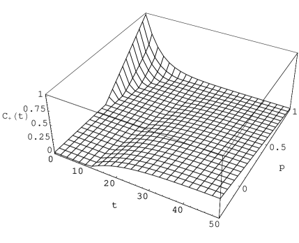
Figure 3: The time evolution of the concurrence $C_{+}$ with different $p$. The pair of atoms is initially prepared in the state $\rho(0)=W_{+}$ and $\gamma=0.1$.

The concurrence can be calculated in a similar way. Before discussing the dynamical behavior of the concurrence, it is useful to consider the long time behavior of the concurrence. With $t\rightarrow\infty$, $\rho_{\pm}(t)$ become

$$\rho_{+s}=\frac{1-p}{4}|{\Psi_{-}}\rangle\langle{\Psi_{-}}|+\frac{3+p}{4}|1,-1\rangle\langle 1,-1|,$$

$$\rho_{-s}=\frac{1+3p}{4}|{\Psi_{-}}\rangle\langle{\Psi_{-}}|+\frac{3-3p}{4}|1,-1\rangle\langle 1,-1|,$$

with the steady entanglements as $C_{+s}=\frac{1-p}{4}$ and $C_{-s}=\frac{1+3p}{4}$, respectively. The above results show that different initial states lead to different steady states with different entanglements. Also from the limit case with $p=1$ one can see that $\Psi_{+}$ is sensitive to the decoherence, while $\Psi_{-}$ is not.

Below we discuss entanglement dynamics in the general case. Fig. 3 and Fig. 4 show the concurrences of $\rho_{\pm}(t)$ as functions of $p$ and $t$. When $p<1/3$, a common characteristic of $\rho_{\pm}(t)$ is that they have no entanglement initially. With time a stable entanglement is formed through the environment. When $p>1/3$, the concurrences of $\rho_{\pm}(t)$ show apparently different time evolution behaviors. For $\rho_{+}(t)$, the entanglement contained in the initial state $W_{+}$ is firstly destroyed by the environment due to the decoherence effect of the environment. The entanglement experiences a “sudden death”[14]. After a finite time duration the entanglement is reconstructed due to the constructive effect of the environment. Physically, the initial contribution to the entanglement in $W_{+}$ comes from the component of $|\Psi_{+}\rangle$. With time, $|\Psi_{+}\rangle$ (i.e. $|1,0\rangle$) approaches to the product state $|1,-1\rangle$ and its entanglement disappears gradually. In this process, the decoherence-free state $|\Psi_{-}\rangle$ is unchanged and the corresponding entanglement gradually dominates the entanglement of $\rho_{+}(t)$ and finally, it reaches the steady state value in the long time limit, i.e., $(1-p)/4$, as mentioned above. Different from $\rho_{+}(t)$, the initial entanglement in $\rho_{-}(t)$ does not decay. This is because the main contribution to the initial entanglement in this case comes from the decoherence-free state $|\Psi_{-}\rangle$. The entanglement induced by the environment is superposed on the initial entanglement. When $p=1$, the Werner state reduces to the pure state $|\Psi_{-}\rangle$ which is independent of time and free from decoherence.

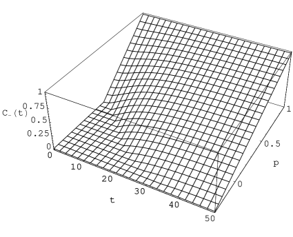
Figure 4: The time evolution of the concurrence $C_{-}$ with different $p$. The pair of atoms is initially prepared in the state $\rho(0)=W_{-}$ and $\gamma=0.1$.

From the special and general analysis above, one sees that the entanglement of the steady state induced by the environment is rooted in the seeds of the entangled decoherence-free states which as components have already been contained in the initial states. This property can be used in choosing a proper initial state to obtain a desired entangled steady state.

4 Entanglement dynamics in a three-qubit system

The three-qubit basis can be constructed from the addition of angular momenta $J_{1},J_{2}$ and $J_{3}$. The representation space is spanned by the common eigenstates of the complete set of commuting operators $\{J_{1,2}^{2},J^{2},J_{z}\}$. The collective basis $|j_{1,2},j,m\rangle$ can be obtained by virtue of the corresponding Clebsch-Gordan coefficients [25]

$$|1,\frac{3}{2},\frac{3}{2}\rangle=|+++\rangle,$$

$$|1,\frac{3}{2},-\frac{3}{2}\rangle=|---\rangle,$$

$$|1,\frac{3}{2},\frac{1}{2}\rangle=\frac{1}{\sqrt{3}}(|++-\rangle+|+-+\rangle+|-++\rangle),$$

$$|1,\frac{3}{2},\frac{-1}{2}\rangle=\frac{1}{\sqrt{3}}(|+--\rangle+|-+-\rangle+|--+\rangle),$$

$$|1,\frac{1}{2},\frac{1}{2}\rangle=\frac{1}{\sqrt{6}}(2|++-\rangle-|+-+\rangle-|-++\rangle),$$

$$|1,\frac{1}{2},\frac{-1}{2}\rangle=\frac{1}{\sqrt{6}}(|+--\rangle+|-+-\rangle-2|--+\rangle),$$

$$|0,\frac{1}{2},\frac{1}{2}\rangle=\frac{1}{\sqrt{2}}(|+-+\rangle-|-++\rangle),$$

$$|0,\frac{1}{2},\frac{-1}{2}\rangle=\frac{1}{\sqrt{2}}(|+--\rangle-|-+-\rangle).$$ (11)

The $J_{\pm}$ act on the collective basis as follows

$$J_{\pm}|j_{1,2},j,m\rangle=\sqrt{j(j+1)-m(m\pm 1)}|j_{1,2},j,m\pm 1\rangle,$$

which are independent of the quantum numbers $j_{1,2}$.

To discuss the entanglement dynamics in the three-qubit system, we use the negativity proposed by Vidal and Werner to quantify the degree of entanglement [19]. The idea of this measure of the entanglement comes from the Peres-Horodecki criterion for the separability of bipartite systems [28]. The negativity was originally introduced to an arbitrary two-qubit state $\rho$ and defined as [19, 29]

$$N(\rho)=-2\sum_{i}\mu_{i}^{-}$$

where $\mu_{i}^{-}$ is the negative eigenvalue of the partial transpose of $\rho$ with respect to the $i-$th qubit, i.e. $\rho^{T_{i}}$. Given a bipartite state one can calculate the partial transpose $\rho^{T_{i}}$ of the density operator. The state is exactly separable if $\rho^{T_{i}}$ is again a positive operator. However, if one of the eigenvalues of $\rho^{T_{i}}$ is negative, the state is entangled [28]. From this viewpoint, the negativity is used to quantify the degree that $\rho^{T_{i}}$ fails to be positive and to represent the strength of quantum correlation between the two subsystems. It was proved that the relation between $C(\rho)$ and $N(\rho)$ is $N(\rho)\geqslant\sqrt{(1-C(\rho))^{2}+C^{2}(\rho)}-[1-C(\rho)]$ for any two-qubit state [29]. The merit of using the negativity to quantify the entanglement is that it allows us to investigate the entanglement properties between part $i$ and the sum of other components in the multipartite system.

Figure 5: The time evolution of the entanglement measured by the negativity $N_{A}$ when the three-atomic state is initially prepared in the state $\rho(0)=|+-+\rangle\langle+-+|$ for $g=1.0$ (solid line), $0.2$ (dashed line), and $0$ (dotted line). The decay constant is chosen to be $\gamma=0.1$.

Similarly, we choose an explicit initial state, e.g., $\rho(0)=|+-+\rangle\langle+-+|$ to discuss the entanglement dynamics in this case. Expanding this initial state in terms of the coupled basis of Eqs. (11)

$$\rho\left(0\right) = |\chi\rangle\langle\chi|,$$

$$|\chi\rangle = \frac{1}{\sqrt{3}}|1,\frac{3}{2},\frac{1}{2}\rangle+\sqrt{\frac{2}{3}}|\psi_{\frac{1}{2}}\rangle,$$

$$|\psi_{\frac{1}{2}}\rangle = \frac{\sqrt{3}}{2}|0,\frac{1}{2},\frac{1}{2}\rangle-\frac{1}{2}|1,\frac{1}{2},\frac{1}{2}\rangle$$ (12)

and using the quantum jump approach, the time-dependent solution of the master equation can be obtained analytically

$$\rho(t) = \frac{e^{-4\gamma t}}{3}|1,\frac{3}{2},\frac{1}{2}\rangle\langle 1,\frac{3}{2},\frac{1}{2}|+\frac{e^{-\gamma t}}{6}|1,\frac{1}{2},\frac{1}{2}\rangle\langle 1,\frac{1}{2},\frac{1}{2}|+\frac{e^{-\gamma t}}{2}|0,\frac{1}{2},\frac{1}{2}\rangle\langle 0,\frac{1}{2},\frac{1}{2}|$$ (13)

$$-\frac{e^{-\frac{5\gamma t}{2}}}{\sqrt{18}}[e^{-i3gt}|1,\frac{3}{2},\frac{1}{2}\rangle\langle 1,\frac{1}{2},\frac{1}{2}|+e^{i3gt}|1,\frac{1}{2},\frac{1}{2}\rangle\langle 1,\frac{3}{2},\frac{1}{2}|]$$

$$+\frac{e^{-\frac{5\gamma t}{2}}}{\sqrt{6}}[e^{-i3gt}|1,\frac{3}{2},\frac{1}{2}\rangle\langle 0,\frac{1}{2},\frac{1}{2}|+e^{i3gt}|0,\frac{1}{2},\frac{1}{2}\rangle\langle 1,\frac{3}{2},\frac{1}{2}|]$$

$$-\frac{e^{-\gamma t}}{\sqrt{12}}[|1,\frac{1}{2},\frac{1}{2}\rangle\langle 0,\frac{1}{2},\frac{1}{2}|+|0,\frac{1}{2},\frac{1}{2}\rangle\langle 1,\frac{1}{2},\frac{1}{2}|]+\frac{1-e^{-\gamma t}}{2}|0,\frac{1}{2},\frac{-1}{2}\rangle\langle 0,\frac{1}{2},\frac{-1}{2}|$$

$$+\frac{4(e^{\gamma t}-1)e^{-4\gamma t}}{3}|1,\frac{3}{2},\frac{-1}{2}\rangle\langle 1,\frac{3}{2},\frac{-1}{2}|+\frac{1-e^{-\gamma t}}{6}|1,\frac{1}{2},\frac{-1}{2}\rangle\langle 1,\frac{1}{2},\frac{-1}{2}|$$

$$-\frac{2e^{-\frac{5\gamma t}{2}}(e^{\gamma t}-1)}{\sqrt{18}}[e^{-i3gt}|1,\frac{3}{2},\frac{-1}{2}\rangle\langle 1,\frac{1}{2},\frac{-1}{2}|+e^{i3gt}|1,\frac{1}{2},\frac{-1}{2}\rangle\langle 1,\frac{3}{2},\frac{-1}{2}|]$$

$$+\frac{2e^{-\frac{5\gamma t}{2}}(e^{\gamma t}-1)}{\sqrt{6}}[e^{-i3gt}|1,\frac{3}{2},\frac{-1}{2}\rangle\langle 0,\frac{1}{2},\frac{-1}{2}|+e^{i3gt}|0,\frac{1}{2},\frac{-1}{2}\rangle\langle 1,\frac{3}{2},\frac{-1}{2}|]$$

$$-\frac{1-e^{-\gamma t}}{\sqrt{12}}[|1,\frac{1}{2},\frac{-1}{2}\rangle\langle 0,\frac{1}{2},\frac{-1}{2}|+|0,\frac{1}{2},\frac{-1}{2}\rangle\langle 1,\frac{1}{2},\frac{-1}{2}|]$$

$$+\frac{1+3e^{-4\gamma t}-4e^{-3\gamma t}}{3}|1,\frac{3}{2},\frac{-3}{2}\rangle\langle 1,\frac{3}{2},\frac{-3}{2}|.$$

In Fig. 5 and Fig. 6 we show the time evolution behavior of the negativity $N_{A}$ and $N_{B}$ corresponding to the partial transpose with respect to the first atom $A$ and second atom $B$, respectively. In the present case, $N_{A}=N_{C},$ where $C$ denotes the third atom. One can see that the system shows a similar property of entanglement production as the two-qubit system. In absence of the direct interactions, the entanglement induced by the environment increases monotonously, then approaches to a stable value at a large time scale for both $N_{A}$ and $N_{B}$. After the interactions are switched on, the oscillation occurs. Moreover, during the evolution of time, this oscillation is suppressed gradually by the environment. From Eq. (13) it is readily seen that the time-dependent solution asymptotically tends to the steady state

$$\rho_{s}=\frac{1}{3}|1,\frac{3}{2},\frac{-3}{2}\rangle\langle 1,\frac{3}{2},\frac{-3}{2}|+\frac{2}{3}|\psi_{\frac{-1}{2}}\rangle\langle\psi_{\frac{-1}{2}}|$$

$$|\psi_{\frac{-1}{2}}\rangle=\frac{\sqrt{3}}{2}|0,\frac{1}{2},\frac{-1}{2}\rangle-\frac{1}{2}|1,\frac{1}{2},\frac{-1}{2}\rangle,$$ (14)

which is a probabilistic mixture of decoherence-free state $|1,\frac{3}{2},\frac{-3}{2}\rangle$ and $|\psi_{\frac{-1}{2}}\rangle$ [27]. In the present three-qubit case, there are two entangled decoherence-free states which contribute to the entanglement of the steady state, i.e. $|0,\frac{1}{2},\frac{-1}{2}\rangle$ and $|1,\frac{1}{2},\frac{-1}{2}\rangle$. It is interesting to note that $\rho_{s}$ is not a simple mixture of three decoherence-free states. It still involves quantum coherence between $|0,\frac{1}{2},\frac{-1}{2}\rangle$ and $|1,\frac{1}{2},\frac{-1}{2}\rangle$. By comparison of the initial state Eqs. (12) with the steady state Eq. (14), we see that although the jump has occurred, i.e. from $|\psi_{\frac{1}{2}}\rangle$ jumps to $|\psi_{\frac{-1}{2}}\rangle$ by the action of $J_{-}$, the superposition coefficients between $|0,\frac{1}{2},j_{z}\rangle$ and $|1,\frac{1}{2},j_{z}\rangle$ are not changed. This is because that the subspaces of $|0,\frac{1}{2},j_{z}\rangle$ and $|1,\frac{1}{2},j_{z}\rangle$ are degenerate under the actions of both the coherent interaction $H_{I}$ and the dissipative operators $J_{\pm}$. Anyway, the steady state $\rho_{s}$ is still an entangled state due to the entangled decoherence-free states contained in $|\psi_{\frac{-1}{2}}\rangle$, which is a linear superposition of the two entangled decoherence-free states.

Figure 6: The time evolution of the entanglement measured by the negativity $N_{B}$ when the three-atomic state is initially prepared in the state $\rho(0)=|+-+\rangle\langle+-+|$ for $g=1.0$ (solid line), $0.2$ (dashed line), and $0$ (dotted line). The decay constant is chosen to be $\gamma=0.1$.

The above discussion in the three-qubit case further confirms the conclusion that the environment has dual nature on the entanglement. Different from the two-qubit case, the Hilbert space of the three-qubit system reduces into three decoupled subspaces $|1,\frac{3}{2},j_{z}\rangle$, $|0,\frac{1}{2},j_{z}\rangle$, and $|1,\frac{1}{2},j_{z}\rangle$, each of which has its own decoherence-free state [27]. Only two of the decoherence-free states are entangled. Under the time evolution, each component in the three subspaces of the initial state approaches its corresponding decoherence-free state. The necessary condition to induce stable entanglement is that the initial state contains the components in the two subspaces with entangled decoherence-free states, i.e. in the subspaces of $|0,\frac{1}{2},j_{z}\rangle$ and $|1,\frac{1}{2},j_{z}\rangle$.

5 Summary

In conclusion, we have investigated a model of quantum register, which is composed of two or three atoms and coupled to a common environment. Using the quantum jump approach, the time-dependent solution of the master equation and the entanglement dynamics of the system are studied analytically and numerically. The dual nature of the common environment on the entanglement and its dissipative dynamical origin are explored in detail based on the eigen solutions of the operator of master equation. On the one hand, due to its induced dissipative term in the master equation, the environment destroys the entanglement induced coherently by the atomic dipole-dipole interactions. On the other hand, due to its induced effective atomic interactions in the master equation, the environment can incoherently induce the entanglement among qubits in the decoherence-free space. The entanglement dynamics studied in the present paper addresses the constructive role of the environment on the entanglement production and suggests to make use of the above positive role to construct an environment-assisted entanglement production in quantum information processing.

References

- [1] M.A. Nielsen and I.L. Chuang, Quantum computation and Quantum Information (Cambridge University Press, Cambridge, UK, 2000).
- [2] P. Štelmachovič and V. Bužek, Phys. Rev. A 70 (2004) 032313.
- [3] A. Hutton and S. Bose, Phys. Rev. A 69 (2004) 042312.
- [4] M.S. Kim, Jinhyoung Lee, D. Ahn, and P.L. Knight, Phys. Rev. A 65 (2002) 040101(R).
- [5] D. Braun, Phys. Rev. Lett. 89 (2002) 277901.
- [6] F. Benatti, R. Floreanini, and M. Piani, Phys. Rev. Lett. 91 (2003) 070402.
- [7] X.X. Yi, C.S. Yu, L. Zhou, and H.S. Song, Phys. Rev. A 68 (2003) 052304.
- [8] J.-H. An, S.-J. Wang, and H.-G. Luo, J. Phys. A: Math. Gen. 38 (2005) 3579.
- [9] F. Benatti, R. Floreanini, Int. J. Mod. Phys. B 19 (2005) 3063.
- [10] F. Benatti, R. Floreanini, Int. J. Quant. Inf. 4, (2006) 395.
- [11] K. Lendi, A. J. van Wonderen, J. Phys. A: Math. Gen. 40 (2007) 279.
- [12] T. Yu and J.H. Eberly, Phys. Rev. B 66 (2002) 193306.
- [13] T. Yu and J.H. Eberly, Phys. Rev. B 68 (2003) 165322.
- [14] T. Yu and J.H. Eberly, Phys. Rev. Lett. 93 (2004) 140404.
- [15] P.J. Dodd and J.J. Halliwell, Phys. Rev. A 69 (2004) 052105 .
- [16] D.F. Walls and G.J. Milburn, Quantum Optics (Springer Verlag, Berlin, Heidelberg, 1994).
- [17] P. Zoller, M. Marte, and D.F. Walls, Phys. Rev. A 35 (1987) 198 .
- [18] W. K. Wootters, Phys. Rev. Lett. 80 (1998) 2245.
- [19] G. Vidal, and R.F. Werner, Phys. Rev. A 65 (2002) 032314.
- [20] M. B. Plenio and P. L. Knight, Rev. Mod. Phys. 70 (1998) 101.
- [21] M.B. Plenio, S.F. Huelga, A. Beige, and P.L. Knight, Phys. Rev. A 59 (1999) 2468.
- [22] R. H. Dicke, Phys. Rev. 93 (1954) 99.
- [23] Z. Ficek, and R. Tanaś, Phys. Rep. 372 (2002) 369.
- [24] R.G. DeVoe and R.G. Brewer, Phys. Rev. Lett. 76 (1996) 2049.
- [25] L. I. Schiff, Quantum Mechanics (McGraw-Hill, New York, 1968).
- [26] C.H. Bennett, D.P. DiVincenzo, J.A. Smolin, and W.K. Wootters, Phys. Rev. A 54 (1996) 3824.
- [27] L.-M. Duan and G.-C. Guo, Phys. Rev. A 58 (1998) 3491.
- [28] A. Peres, Phys. Rev. Lett. 77 (1996) 1413.
- [29] A. Miranowicz and A. Grudka, Phys. Rev. A 70 (2004) 032326.