Recurrence Tracking Microscope

Abstract

In order to probe nanostructures on a surface we present a microscope based on the quantum recurrence phenomena. A cloud of atoms bounces off an atomic mirror connected to a cantilever and exhibits quantum recurrences. The times at which the recurrences occur depend on the initial height of the bouncing atoms above the atomic mirror, and vary following the structures on the surface under investigation. The microscope has inherent advantages over existing techniques of scanning tunneling microscope and atomic force microscope. Presently available experimental technology makes it possible to develop the device in the laboratory.

I INTRODUCTION

In 1982, Binnig and Rohrer used quantum tunneling phenomenon as a probe to study nano-structures on a surface binn1 . The idea led to the development of Scanning Tunneling microscope (STM) and won the inventors Nobel prize in physics in 1986. Later, the inventors of the STM designed the Atomic Force microscope (AFM) binn2 . In this paper we present a microscope based on quantum recurrence phenomena to probe nano-structures on a surface with atomic size resolution, and therefore appropriately name the device as Recurrence tracking microscope (RTM).

Recurrence Tracking Microscope is in many ways advantageous over existing techniques of STM and AFM: (i) It probes material surfaces of all kinds ranging from conductors to insulators; (ii) It investigates surfaces comprising impurities without observing the impurity atoms as extra surface structures. STM, however, has a drawback as it observes extra surface structures for the impurity atoms meyer ; (iii) In dynamical operational mode, RTM provides information about a surface with periodic structures in the simplest manner saifRTM . Due to the periodicity of the structures on the surface, the cantilever oscillates with a finite frequency. The oscillations of the cantilever and then of the atomic mirror, appear as a periodically changing force to the bouncing atoms. As a result the time of recurrence is modified and the modification factor stores the information of the periodicity of the surface structures.

Quantum recurrences of a atomic wave packet in the absence Robinett and in the presence SaifPR of an oscillating surface are well understood. The phenomena have been realized as well experimentally kn:park . The increased dynamical stability in the surface traps needed to develop RTM has extended the limits of the experiments from a few bounces kn:kase ; Aminoff ; EdHinds1 to even realize Bose-Einstein condensation of atoms using an optical reflecting surface Rychtarik and a magnetic film EdHinds2 .

In Sec. II, we introduce the experimental setup of the Recurrence tracking microscope (RTM). In Sec.III, and IV we explain the static and dynamical modes, respectively.

II THE EXPERIMENTAL MODEL

In order to realize the Recurrence Tracking microscope, we place a cloud of cold atoms, trapped in a magneto-optic trap, above an atomic mirror. The mirror for the atomic de Broglie waves is obtained by the total internal reflection of a monochromatic laser light from a dielectric film. The dielectric film is attached to the cantilever, which has its other end above the surface under investigation, as shown in Fig. 1.

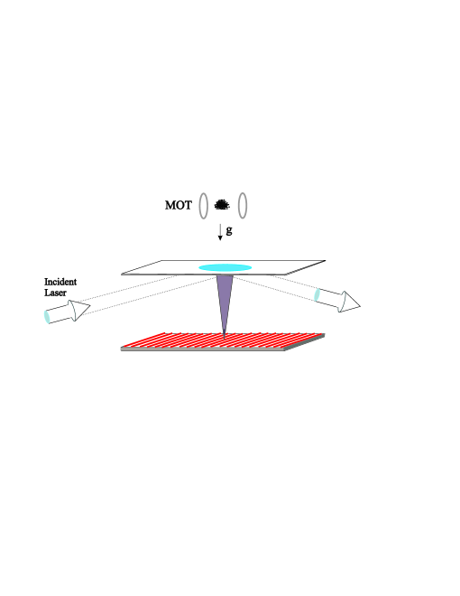
Figure 1: Experimental setup of the Recurrence Tracking Microscope: A cloud of atoms is trapped and cooled in a magneto optical trap (MOT) down to the micro-Kelvin scale. The MOT is placed at a certain height above the evanescent wave atomic mirror. The mirror for the atoms results due to the total internal reflection of the incident laser light field from the surface of the dielectric film. Thus an evanescent wave field is produced on the surface which has polarization inside the plane of the reflection. The dielectric film is connected to a cantilever, which has its other end above the surface under investigation. We consider the atomic dynamics along $z$-axis, normal to the surface of the mirror.

Figure 2: The net potential seen by an atom in the presence of an optical field and a gravitational field (left), and its evolution over two bounces (right): On switching off the MOT, the atom starts its motion from an initial height $z_{0}$ at time $t=0$. It moves under the influence of the linear gravitational potential, $V_{gr}=mgz$, towards the evanescent wave atomic mirror and experiences a constant attractive force. Close to the surface of the mirror the effect of the evanescent light field is dominant. The atom, due to the exponentially increasing optical potential $V_{opt}=V_{0}e^{-\kappa z}$, experiences an exponentially increasing repulsive force and bounces back. Both the potentials together make an atomic trampoline or a gravitational cavity for the atom. On the right, we display the evolution of the material wave packet over two bounces in position space as a function of time.

At the onset of the experiment, the magneto-optic trap is switched off, and we let the atoms move towards the atomic mirror under the influence of the gravitational field. We consider that the frequency, $\nu$, of the optical field which makes the atomic mirror is tuned far from the transition frequency, $\nu_{0}$, between any two atomic levels. The probability of spontaneous emission kn:seif is $P_{sp}=\gamma\frac{\Omega^{2}_{max}}{4\delta^{2}}\tau_{ref},$ where, $\delta=\nu-\nu_{0}$ is the amount of atom-field detuning, $\gamma$ is the decay constant of the higher state, and $\tau_{ref}=2/\kappa v_{z}$ is the characteristic time of the atom-field interaction during the process of reflection off the atomic mirror. The quantity $v_{z}$ describes the velocity of the atom along the gravitational field in the $z$ direction. Hence, for a large detuning, $\delta$, the probability of finding the atom in the excited state becomes smaller. For the reason it becomes possible to neglect spontaneous emission in experiments under the condition of a large atom-field detuning kn:sten .

The atomic mirror is made up of an evanescent wave field, ${\bf E}(z)$, which varies with the position, as a consequence the Rabi frequency of the atom, $\Omega={\bf d}\cdot{\bf E}(z)/\hbar$, becomes position dependent as well. Hence, $\Omega_{max}$ expresses the maximum Rabi frequency seen by the atom at its turning point on the surface of the mirror. Here, the light shift due to the external field compensates the kinetic energy of the atom of mass $m$, that is, $\frac{\hbar\Omega_{max}^{2}}{4\delta}=mv_{z}^{2}/2.$

Near the dielectric surface, the atoms observe an exponentially increasing repulsive force, $F_{opt}=V_{o}\kappa e^{-\kappa z}$, as they are detuned to the blue, that is $\nu$ is larger than $\nu_{0}$. Here, $\kappa^{-1}$ defines the decay length of the atomic mirror. Therefore, away from the mirror the repulsive optical force is negligible. However, due to the gravitational field the atom experiences a constant gravitational force $F_{g}=-mg$, and is pushed towards the mirror. Hence, the atom undergoes a bounded motion in the presence of the optical potential and the gravitational potential together, as shown in Fig. 2. The bounded atomic dynamics in so-generated gravitational cavity or atomic trampoline is controlled by the effective Hamiltonian, $H=p^{2}/2m+mgz+V_{0}e^{-\kappa z}.$ Here, $p$ describes the center-of-mass momentum along the $z$ axis. Moreover, $m$ indicates mass of the atom, and $g$ expresses the constant gravitational acceleration.

III STATIC MODE OF OPERATION

A material wave packet, with a finite width in energy, undergoes constructive and destructive interferences in its evolution in time. In quantum mechanical evolution, interference plays an important role and manifests itself in quantum recurrences. The wave-packet follows classical evolution for a short duration of time and reappears after a classical period. However, after a few classical periods it spreads all over the available space following wave mechanics and collapses. However, due to quantum dynamics it rebuilds itself after a certain evolution time. The phenomenon is named as the quantum revival of the wave packet and the time at which it reappears after a collapse is quantum revival time. At the fractions of the quantum revival time, we find partial appearance of the initially propagated wave packet. Therefore, these times are called fractional revival times Robinett ; SaifPR .

We propagate an atomic wave packet, $|\psi\rangle$, which has a distribution over eigen states with width $\Delta n$, centered at mean quantum number $n_{0}$. We express the wave packet as a superposition in the Hilbert space defined by the eigen states of the net potential, that is, $|\psi\rangle=\sum_{n}c_{n}|\phi_{n}\rangle,$ where, $c_{n}$ describes the probability amplitude of the wave packet in the $n$th state. Moreover, $|\phi_{n}\rangle$ are the eigen states of the net potential, such that, ${\hat{H}}|\phi_{n}\rangle=E_{n}|\phi_{n}\rangle$, where ${\hat{H}}$ is the time independent Hamiltonian of the system. Since there is no explicit time dependence the wave packet, after a propagation time $t$, appears as

$$|\psi(t)\rangle=e^{-iHt/\hbar}|\psi_{n}(t=0)\rangle=\sum_{n}c_{n}e^{-iE_{n}t/\hbar}|\phi_{n}\rangle.$$ (1)

In order to study the evolution of the wave packet in the potential we calculate the autocorrelation function, $C(t)$, defined as

$$C(t)=\langle\psi(0)|\psi(t)\rangle\equiv\sum_{n}|c_{n}|^{2}\exp\{-iE_{n}t/\hbar\}.$$ (2)

Here, we have used the property of orthonormality of the eigen states. We consider that $|c_{n}|^{2}$ corresponds to a distribution narrowly peaked around $n_{0}$. Therefore, we may write Eq. (2) by using Taylor’s expansion for energy $E_{n}$ around $n_{0}$. This leads us to calculate the times, $T^{(j)}_{0}$, at which the system exhibits recurrences. Here $j$ is an integer. We write these times as, $T^{(j)}_{0}=\frac{2\pi\hbar}{\frac{1}{j!}|E_{n}^{(j)}|}$, where, $E_{n}^{(j)}\equiv\left.\frac{\partial^{j}E_{n}}{\partial n^{j}}\right|_{n=n_{0}}$ describes the $j$th derivative of the energy with respect to the principal quantum number $n$, calculated at $n=n_{0}$. The first term

$$T^{(1)}_{0}=2\pi\hbar\left(\left|\frac{\partial E_{n}}{\partial n}\right|_{n=n_{0}}\right)^{-1}=2\pi\left(\left|\frac{\partial E_{I}}{\partial I}\right|_{I=I_{0}}\right)^{-1}$$ (3)

is independent of $\hbar$ in action-angle space and corresponds to the classical period of the wave packet. Here, $I$ ($=n\hbar$) is the classical action, therefore, $I_{0}=n_{0}\hbar$. However, the second term of the expansion

$$T^{(2)}_{0}=2\pi\hbar\left(\frac{1}{2!}\left|\frac{\partial^{2}E_{n}}{\partial n^{2}}\right|_{n=n_{0}}\right)^{-1}=2\pi\left(\frac{\hbar}{2!}\left|\frac{\partial^{2}E_{n}}{\partial I^{2}}\right|_{I=I_{0}}\right)^{-1},$$ (4)

yields the quantum mechanical revival time of the wave packet in the potential.

In order to calculate the quantum revival time for the atom in RTM, we approximate the net potential, made up by the optical potential and the gravity, as a triangular well potential chen1 . The energy of the triangular well potential is defined as

$$E_{n}=\left(\frac{m\hbar^{2}g^{2}}{2}\right)^{1/3}z_{n}.$$ (5)

Here, $z_{n}$’s are negative zeros of Airy function, and can be defined kn:abra as $z_{n}=f\left(\frac{3\pi}{2}(n-1/4)\right)$, where $f(\zeta)=\zeta^{2/3}\left(1+\frac{5}{48\zeta^{2}}-\frac{5}{36\zeta^{4}}+\cdots\right).$ In case of large $n$, we may reduce $z_{n}$ to $z_{n}\cong(3n\pi/2)^{2/3}$ which provides the eigen energies of the system, as $E_{n}\cong\frac{m^{1/3}}{2}\left(3n\pi\hbar g\right)^{2/3}.$ With the knowledge of $E_{n}$ at hand the quantum revival time, $T^{(2)}_{0}$, is obtained with the help of Eq. (4), such that

$$T^{(2)}_{0}=\frac{16E_{n_{0}}^{2}}{m\pi\hbar g^{2}},$$ (6)

where, $E_{n_{0}}$ is the initial mean energy of the material wave packet.

Hence, in order to probe a surface which has arbitrary structures, we use the quantum recurrence tracking microscope in static mode. We let the atom fall on the static atomic mirror without moving the surface under investigation. In its evolution over the atomic mirror for a certain fixed position of the cantilever the atom displays quantum revival at quantum revival time, $T^{(2)}_{0}$, as given in Eq. (6).

As we slightly move the surface under study, the position of the cantilever changes following the surface structures. This changes the initial distance between the atomic mirror and the bouncing atom. This leads to a different initial energy $E_{n_{0}}$ for the atom, and thus a different revival time, $T^{(2)}_{0}$. For each new experimentally calculated $T^{(2)}_{0}$, we calculate the corresponding $E_{n_{0}}$, which leads to the knowledge of the structures on the surface being probed.

IV DYNAMICAL MODE OF OPERATION

In case the surface under study has periodic nano-structures, we find periodic spatial modulation of the atomic mirror as we move the surface horizontally below the cantilever. The lower tip of the cantilever follows the surface structures and introduces spatial modulation to the atomic mirror at its other end. Hence, the dynamics of an atom is controlled by an explicitly time dependent Hamiltonian, $H=\frac{P^{2}}{2m}+mgz+V_{0}e^{-k(z-a\sin\omega t)}$, where, $a$ describes the amplitude of the spatial modulation which corresponds to the height of the periodic structures and $\omega$ defines the frequency at which the structures appear.

In the presence of the spatial modulation of the atomic mirror, the bouncing atom displays collapse and revival after a definite period of time. We saif calculate the time of the quantum revival as

$$T^{(2)}_{\lambda}=T^{(2)}_{0}\left[1-\frac{1}{8}\left(\frac{mga}{E_{n_{0}}}\right)^{2}\frac{3(1-r)^{2}+\tilde{a}^{2}}{[\left(1-r\right)^{2}-\tilde{a}^{2}]^{3}}\right],$$ (7)

where, $r\equiv(E_{N}/E_{n_{0}})^{1/2}$ and $\tilde{a}=r^{2}\hbar\omega/4E_{n_{0}}$ are dimensionless parameters. The time $T^{(2)}_{0}$, expressed in Eq. (6), defines the quantum revival time for the atomic wave packet in the absence of the modulation of the atomic mirror, that is, on the static surface. The time of the quantum revival in the presence of modulation, as given in Eq. (7), depends upon the frequency, $\omega$, and the height of the periodic structures, $a$.

We measure $a$ by considering that the material wave packet is released from the MOT, with a large initial mean energy $E_{n_{0}}$, such that $(1-r)^{2}>\tilde{a}^{2}$. Hence, the time of the quantum revival $T^{(2)}_{\lambda}$ becomes,

$$T^{(2)}_{\lambda}=T^{(2)}_{0}\left[1-\frac{3}{8}\left(\frac{mga}{E_{n_{0}}}\right)^{2}\frac{1}{\left(1-r\right)^{4}}\right],$$

which provides the value of $a$, expressing the height of the periodic structures as,

$$a=\sqrt{\frac{8}{3}}\frac{E_{n_{0}}}{mg}\left(1-r\right)^{2}\left[1-\frac{T^{(2)}_{\lambda}}{T^{(2)}_{0}}\right]^{1/2}.$$ (8)

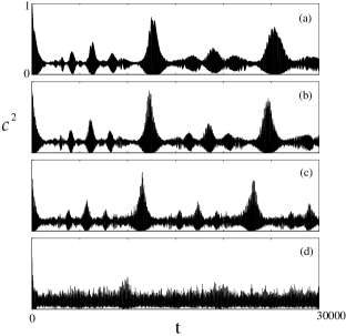
Figure 3: We propagate a cloud of Cs atoms centered at mean quantum number $n_{0}=176.16$, with a width $\Delta z=0.28\mu m$, from a height $z_{0}=20.1\mu m$ saif . We calculate the time of quantum revivals numerically for different values of initial modulations. We substitute these values in Eqs. (8) and (10) and get the corresponding values of $a$ as (a) 0, (b) 11.4$nm$ (c) 23$nm$ (d) 46$nm$ and frequency as $\omega=2\pi$x$1KHz$ kn:sten . If the surface under study is moved below cantilever with a velocity of $1\mu m/sec$ the spacing between the surface structures is noted as $1nm$.

Knowledge of the value of $a$ helps us to find the frequency, $\omega$, of the appearance of the periodic structures. We may express Eq. (7) as,

$$\left[\left(1-r\right)^{2}-\tilde{a}^{2}\right]^{3}\alpha_{T}-\left[3\left(1-r\right)^{2}+\tilde{a}^{2}\right]=0,$$ (9)

where,

$$\alpha_{T}=8\left(\frac{E_{n_{0}}}{mga}\right)^{2}\left[1-\frac{T^{(2)}_{\lambda}}{T^{(2)}_{0}}\right].$$ (10)

We find the values of $T^{(2)}_{0}$ and $T^{(2)}_{\lambda}$ experimentally, and substitute them in Eq. (10) to obtain the value of $\alpha_{T}$. Thus, we find $\tilde{a}$ as the roots of Eq. (9), which yields the frequency $\omega$, as $\omega=4E_{n_{0}}\tilde{a}/r^{2}\hbar$. Hence, the measurement of the quantum revival times, $T^{(2)}_{0}$ and $T^{(2)}_{\lambda}$, and the height $a$, help to measure the frequency, $\omega$. This immediately leads us to calculate the spacing between the surface structures as we know the velocity at which the surface is moved horizontally below the cantilever.

We calculate the square of the auto correlation function and display our numerical results in Fig. 3. We consider a cloud of cesium atoms initially in a Gaussian distribution centered at mean quantum number $n_{0}=176.16$, with a width $\Delta z=0.28\mu m$, which is propagated from an initial height $z_{0}=20.1\mu m$ Ovchinnikov1997 . We calculate the time of quantum revivals numerically for different modulations of the atomic mirror. On substituting the values in Eqs. (8) and (10) we obtain the height $a$, and the frequency $\omega$ at which the periodic structures appear on the surface.

We suggest that the Recurrence tracking microscope opens new horizons to study and incorporate effects of atomic coherence and interference. As discussed above, the RTM has clear advantages over STM and AFM. The bouncing atoms reflect back above the dielectric surface and do not influence the dielectric surface or cantilever, this may increase the stability of the system. The ability to scan all kind of surfaces is another credit to the device. In addition, RTM in dynamical mode scans the periodic structures more swiftly saifpatent .

V ACKNOWLEDGMENT

The author submits his thanks to Prof. Pierre Meystre for his hospitality at the Department of Physics, the University of Arizona.

References

- (1) G. Binnig, H. Rohrer, Ch. Gerber and E. Weibel, Phys. Rev. Lett. 49, 57 (1982).
- (2) G. H. Binnig, and H. Rohrer, IBM J. Res. Dev. 30, 355 (1986).
- (3) E. Meyer, H. J. Hug, and R. Bennewitz, Scanning Probe Microscope (Springer-Verlag Berlin, 2004).
- (4) F. Saif, and A. Khalique, in Proceedings of the National Symposium on Physics in Industry, Karachi 2001, edited by M. Ahmad and A. ul Haq, p. 15.
- (5) R. W. Robinett, Phys. Rep. 392, 1 (2004).
- (6) Farhan Saif, Phys. Rep. 419, 207 (2005); F. Saif, Phys. Rep. 425, 369 (2006).
- (7) Parker J. and C. R. Stroud, Jr., Phys. Rev. Lett. 56, 716 (1986); J. Wals, H. H. Fielding, J. F. Christian, L. C. Snoek, W. J. van der Zande, and H. B. van Linden van den Heuvell, Phys. Rev. Lett. 72, 3783 (1994).
- (8) M. A. Kasevich, D. S. Weiss, and S. Chu, Opt. Lett. 15, 607 (1990).
- (9) C. G. Aminoff, A. M. Steane, P. Bouyer, P. Desbiolles, J. Dalibard, and C. Cohen Tannoudji, Phys. Rev. Lett. 71, 3083 (1993).
- (10) Roach T. M., H. Abele, M. G. Boshier, H. L. Grossman, K. P. Zetie, and E. A. Hinds, Phys. Rev. Lett. 75, 629 (1995); Hughes I. G., P. A. Barton, M. G. Boshier and E. A. Hinds, J. Phys. B 30, 647 (1997); Hughes I. G., P. A. Barton, and E. A. Hinds, J. Phys. B 30, 2119 (1997); Saba C. V., P. A. Barton, M. G. Boshier, I. G. Hughes, P. Rosenbusch, B. E. Sauer and E. A. Hinds, Phys. Rev. Lett. 82 468 (1999); E. A. Hinds and I. G. Hughes, J. Phys. D 32, R119 (1999); I. G. Hughes, T. Darlington, and E. A. Hinds, J. Phys. B 34, 2869 2001; P. Rosenbusch, B.V. Hall, I. G. Hughes, C. V. Saba, and E. A. Hinds, Appl. Phys. B 70, 709 (2000); M. Key, I. G. Hughes, W. Rooijakkers, B. E. Sauer, E. A. Hinds, D. J. Richardson, and P. G. Kazansky, Phys. Rev. Lett. 84, 1371 (2000); P. Rosenbusch, B. V. Hall, I. G. Hughes, C. V. Saba, and E. A. Hinds, Phys. Rev. A 61, 031404R (2000).
- (11) D. Rychtarik, B. Engeser, H.-C. N gerl, and R. Grimm, Phys. Rev. Lett. 92, 173003 (2004).
- (12) C. D. J. Sinclair, E. A. Curtis, I. L. Garcia, J. A. Retter, B. V. Hall, S. Eriksson, B. E. Sauer, and E. A. Hinds Phys. Rev. A 72, 031603 (2005)
- (13) W. Seifert, R. Kaiser, A. Aspect, and J. Mlynek, Opt. Commun. 111 (1994) 566.
- (14) A. Steane, P. Szriftgiser, P. Desbiolles and J. Dalibard: Phys. Rev. Lett. 74, 4972 (1995); Wallis H., Phys. Rep. 255, 203 (1995).
- (15) Wen-Yu Chen and G. J. Milburn, Phys. Rev. A 51, 2328 (1995).
- (16) M. Abramowitz and I.A. Stegun, Handbook of Mathematical Functions, (Dover, New York, 1992).
- (17) F. Saif, and M. Fortunato, Phys. Rev. A 65 013401 (2002) 013401.
- (18) F. Saif, J. Opt B: Quantum Semiclass. Opt. 7 S116 (2005);
- (19) Yu. B. Ovchinnikov, I. Manek, and R. Grimm, Phys. Rev. Lett. 79 (1997) 2225.
- (20) F. Saif, patent pending.