Quantum Reversibility and Echoes in Interacting Systems

Abstract

In Echo experiments, imperfect time-reversal operations are performed on a subset of the total number of degrees of freedom. To capture the physics of these experiments, we introduce a partial fidelity ${\cal M}_{\rm B}(t)$, the Boltzmann echo, where only part of the system’s degrees of freedom can be time-reversed. We present a semiclassical calculation of ${\cal M}_{\rm B}(t)$. We show that, as the time-reversal operation is performed more and more accurately, the decay rate of ${\cal M}_{\rm B}(t)$ saturates at a value given by the decoherence rate of the controlled degrees of freedom due to their coupling to uncontrolled ones. We connect these results with NMR spin echo experiments.

One of the central problems faced by the founders of statistical physics in the last decades of the nineteenth century was to reconcile the time-asymmetric evolution of macroscopic systems with time-symmetric microscopic dynamics loschmidt . They came up with a probabilistic solution to this irreversibility paradox. Macroscopic states, they argued, are superpositions of an enormous amount of microscopic states, the majority of them evolving in accordance with the second law of thermodynamics. The likelihood that a macroscopic state violates the second law of thermodynamics is thus minute, typically exponentially small in the number of atoms it contains. Irreversibility at the macroscopic level follows “by assuming a very improbable (i.e. with a very low entropy) initial state of the entire universe” lebowitz ; boltzmann . This mechanism works equally well in either quantum or classical systems.

Simple mechanisms of irreversibility already exist at the microscopic level in chaotic (in particular mixing) classical systems with few degrees of freedom. As a matter of fact, mixing ensures that, after a sufficiently long evolution time, two initially well separated phase-space distributions will evenly fill phase-space cells of any given size. Since phase-space points can never be located with infinite precision, irreversibility sets in after mixing has occurred on a scale smaller than the phase-space resolution scale. This mechanism cannot be carried over to quantum systems, however, mostly because the Schrödinger time-evolution is unitary, in either real- or momentum-space. Microscopic quantum systems are generically stable under time-reversal, even when their classical counterpart is irreversible dima . Peres instead suggested to investigate quantum irreversibility at the microscopic level through the fidelity

$${\cal M}_{\rm L}(t)=\left|\left\langle\psi_{0}\left|\exp[iHt]\exp[-iH_{0}t]\right|\psi_{0}\right\rangle\right|^{2},$$ (1)

with which a quantum state $\psi_{0}$ can be reconstructed by inverting the dynamics after a time $t$ with a perturbed Hamiltonian $H=H_{0}+\Sigma$ peres . Because of its connection with the gedanken time-reversal experiment proposed by Loschmidt in his argument against Boltzman’s H-theorem loschmidt , ${\cal M}_{\rm L}(t)$ has been dubbed the Loschmidt Echo by Jalabert and Pastawski Jal01 .

Echo experiments abound in nuclear magnetic resonance hahn ; nmr , optics kurnit , atomic davidson , and condensed matter physics nakamura . Fundamentally, they are all based on the same principle of a sequence of electromagnetic pulses whose purpose it is to reverse the sign of the Hamiltonian, $H_{0}\rightarrow-H_{0}$, by means of effective changes of coordinate axes hahn . Imperfections in the pulse sequence result instead in $H_{0}\rightarrow-H_{0}-\Sigma$, and one therefore expects the Loschmidt Echo to capture the physics of the experiments. This line of reasoning however neglects the fact that the time-reversal operation affects at best only part of the system, for instance because the system is composed of so many degrees of freedom, that the time arrow can be inverted only for a fraction of them. This is generically the case, as any system is coupled to an external, uncontrolled environment. To capture the physics of echo experiments one thus has to take into account that (i) the system decomposes into two interacting subsystems 1 and 2; (ii) the initial state of the controlled subsystem 1 is prepared, i.e. well defined, and its final state is measured and compared to the initial one; (iii) both the initial and final states of the uncontrolled subsystem 2 are unknown; (iv) the Hamiltonian of system 1 is time-reversed with some tunable accuracy, however both the Hamiltonian of system 2 and the interaction between the two subsystems are uncontrolled. We therefore propose to investigate the physics of echo experiments by means of the following partial fidelity (we set $\hbar\equiv 1$)

$${\cal M}_{\rm B}(t)=\Big{\langle}\big{\langle}\psi_{1}\big{|}{\rm Tr}_{2}\left[e^{-{\it i}{\cal H}_{\rm b}t}e^{-{\it i}{\cal H}_{\rm f}t}\rho_{0}e^{{\it i}{\cal H}_{\rm f}t}e^{{\it i}{\cal H}_{\rm b}t}\right]\big{|}\psi_{1}\big{\rangle}\Big{\rangle},$$ (2)

where the forward and backward (partially time-reversed) Hamiltonians read

$${\cal H}_{\rm f} = H_{1}\otimes I_{2}+I_{1}\otimes H_{2}+{\cal U}_{\rm f},$$ (3a)

$${\cal H}_{\rm b} = -[H_{1}+\Sigma_{1}]\otimes I_{2}+I_{1}\otimes[H_{2}+\Sigma_{2}]+{\cal U}_{\rm b}.$$ (3b)

The experiment starts with an initial density matrix $\rho_{0}=|\psi_{1}\rangle\langle\psi_{1}|\otimes\rho_{2}$, which is propagated forward in time with ${\cal H}_{\rm f}$. After a time $t$, we invert the dynamics of system 1. The imperfection in that time-reversal operation is modelled by $\Sigma_{1}$, while $\Sigma_{2}$ allows for system 2 to be affected by this operation (we will see below that tracing over the degrees of freedom of system 2 makes ${\cal M}_{\rm B}(t)$ independent of either $H_{2}$ or $\Sigma_{2}$). We leave open the possibility that the interaction between the two systems is affected by the time-reversal operation, i.e. ${\cal U}_{\rm f}$ may or may not be equal to ${\cal U}_{\rm b}$. Because one has no control over system 2, the corresponding degrees of freedom are traced out. For the same reason, the outmost brackets in Eq. (2) indicate an average over $\rho_{2}$. We name ${\cal M}_{\rm B}(t)$ the Boltzmann echo to stress its connection to Boltzmann’s counterargument to Loschmidt that time cannot be inverted for all components of a system with many degrees of freedom.

In this article, we present a semiclassical calculation of the Boltzmann echo for two classically chaotic subsystems along the lines of Refs.Jal01 ; Jac04 ; Pet05 , and compare our results with those obtained from a Random Matrix Theory (RMT) treatment of the problem. Our main result is that, in the regime of classically weak but quantum mechanically strong imperfection $\Sigma_{1}$ and coupling ${\cal U}_{\rm f,b}$, ${\cal M}_{\rm B}(t)$ is the sum of two exponentials

$${\cal M}_{\rm B}(t)\simeq\exp\left[-\left(\Gamma_{\Sigma_{1}}+\Gamma_{\rm f}+\Gamma_{\rm b}\right)t\right]+\alpha_{1}\exp\left[-\lambda_{1}t\right].$$ (4)

Here, $\alpha_{1}$ is a weakly time-dependent prefactor, $\lambda_{1}$ is the classical Lyapunov exponent of system 1, and $\Gamma_{\Sigma_{1}}$ and $\Gamma_{\rm f,b}$ are given by classical correlators for $\Sigma_{1}$ and ${\cal U}_{\rm f,b}$ respectively (see below). Equivalently, they can be regarded as the golden rule width of the Lorentzian broadening of the levels of $H_{1}$ induced by $\Sigma_{1}$ and ${\cal U}_{\rm f,b}$ respectively Jac01 . Together with the one- and two-particle level spacings $\delta_{1,2}$ and bandwidths $B_{1,2}$, they define the range of validity of the semiclassical approach as $\delta_{1}<\Gamma_{\Sigma_{1}}<B_{1}$, $\delta_{2}<\Gamma_{\rm f,b}<B_{2}$ Jac01 ; Jac04 ; Pet05 . The second term on the right-hand side of Eq. (4) exists exclusively for a classically meaningful initial state $\psi_{1}$ such as a Gaussian wavepacket or a position state, but the first term is much more generic. It emerges from both a semiclassical or a RMT treatment and does not depend on the initial preparation $\psi_{1}$ of system 1. Other regimes of decay exist, which we here mention for the sake of completeness. For quantum mechanically weak $\Gamma_{\Sigma_{1}}\ll\delta_{1}$ and $\Gamma_{\rm f,b}\ll\delta_{2}$, one has a Gaussian decay,

$${\cal M}_{\rm B}(t)=\exp\left[-\left(\overline{\Sigma_{1}^{2}}/4+\overline{{\cal U}_{\rm f}^{2}}/2+\overline{{\cal U}_{\rm b}^{2}}/2\right)t^{2}\right],$$ (5)

in term of the typical squared matrix elements of $\Sigma_{1}$ and ${\cal U}_{\rm f,b}$. Also, at short times a parabolic decay of ${\cal M}_{\rm B}(t)$ prevails for any coupling strength. Finally, if system 1 is integrable, the decay of ${\cal M}_{\rm B}(t)$ is power-law in time.

The equivalence between Boltzmann and Loschmidt echoes is broken by $\Gamma_{\rm f,b}$, the decoherence rate of system 1 induced by the coupling to system 2 (or by $\overline{{\cal U}_{\rm f,b}^{2}}$ at weak interaction). Skillfull experimentalists can thus investigate decoherence in echo experiments with weak time-reversal imperfection $\Sigma_{1}$ for which $\Gamma_{\Sigma_{1}}\ll\Gamma_{\rm f,b}$, and thus ${\cal M}_{\rm B}(t)\simeq\exp[-(\Gamma_{\rm f}+\Gamma_{\rm b})t]$ (or ${\cal M}_{\rm B}(t)\simeq\exp[-(\overline{{\cal U}_{\rm f}^{2}}+\overline{{\cal U}_{\rm b}^{2}})\;t^{2}/2]$ at weak interaction) as $\Sigma_{1}$ is reduced. This might well be the explanation for the experimentally observed $\Sigma_{1}$-independent decay of polarization echoes levstein .

We now present our calculation. As starting point, we take chaotic one-particle Hamiltonians $H_{1,2}$, and a smooth interaction potential ${\cal U}$ which depends only on the distance between the particles. We assume that it is characterized by a typical classical length scale, which in particular is larger than the de Broglie wavelength $\sigma$ of particle 1. For pedagogical reasons, we take narrow Gaussian wavepackets for the initial state of both particles, $\psi_{i}({\bf q})=\langle{\bf q}|\psi_{i}\rangle=(\pi\sigma^{2})^{-d_{i}/4}\exp[{\it i}{\bf p}_{i}\cdot({\bf q}-{\bf r}_{i})-|{\bf q}-{\bf r}_{i}|^{2}/2\sigma^{2}]$. We note however that within our semiclassical approach, more general states can be taken for the uncontrolled system 2, such as random pure states $\rho_{2}=\sum_{\alpha\beta}a_{\alpha}a_{\beta}^{\ast}|\phi_{\alpha}\rangle\langle\phi_{\beta}|$, random mixtures $\rho_{2}=\sum_{\alpha}|a_{\alpha}|^{2}|\phi_{\alpha}\rangle\langle\phi_{\alpha}|$ or thermal mixtures $\rho_{2}=\sum_{n}\exp\left[-\beta E_{n}\right]|n\rangle\langle n|$. Arbitrary initial states for both subsystems can be considered within the RMT approach.

From Eqs. (2) and (3) we can rewrite ${\cal M}_{\rm B}(t)$ as

$${\cal M}_{\rm B}(t) = \int{\rm d}{\bf z}_{2}\;\;\;\Bigg{|}\int\prod_{i=1}^{2}{\rm d}{\bf x}_{i}\prod_{j=1}^{3}{\rm d}{\bf q}_{j}\;\psi_{1}({\bf q}_{1})\psi_{2}({\bf q}_{2})\psi^{\dagger}_{1}({\bf q}_{3})\left\langle{\bf q}_{3},{\bf z}_{2}\left|e^{-{\it i}{\cal H}_{\rm b}t}\right|{\bf x}_{1},{\bf x}_{2}\right\rangle\left\langle{\bf x}_{1},{\bf x}_{2}\left|e^{-{\it i}{\cal H}_{\rm f}t}\right|{\bf q}_{1},{\bf q}_{2}\right\rangle\Bigg{|}^{2}.$$ (6)

We next introduce the semiclassical propagators ($a={\rm f,b}$ labels forward or backward evolution; $\epsilon^{(f)}=-\epsilon^{(b)}=1$),

$$\left\langle{\bf x}_{1},{\bf x}_{2}\left|e^{-{\it i}{\cal H}_{a}t}\right|{\bf q}_{1},{\bf q}_{2}\right\rangle\;=\sum_{s_{1},\,s_{2}}{\cal C}_{s_{1},s_{2}}^{1/2}\exp\left[{\it i}\left\{\epsilon^{(a)}S^{(a)}_{s_{1}}({\bf q}_{1},{\bf x}_{1};t)+S^{(a)}_{s_{2}}({\bf q}_{2},{\bf x}_{2};t)+{\cal S}^{(a)}_{s_{1},s_{2}}({\bf q}_{1},{\bf x}_{1};{\bf q}_{2},{\bf x}_{2};t)\right\}\right],$$ (7)

which are expressed as sums over pairs of classical trajectories, labeled $s_{i}$ ($l_{i}$) for particle $i$ connecting ${\bf q}_{i}$ to ${\bf x}_{i}$ in the time $t$ with dynamics determined by $H_{i}$ or $H_{i}+\Sigma_{i}$. Under our assumption of a classically weak coupling, classical trajectories are only determined by the one-particle Hamiltonians. Each pair of paths gives a contribution containing one-particle action integrals denoted by $S_{s_{i}}$ (where we included the Maslov indices) and two-particle action integrals ${\cal S}^{({\rm f,b})}_{s_{1},s_{2}}=\int_{0}^{t}{\rm d}\tau{\cal U}_{{\rm f,b}}[{\bf q}_{s_{1}}(\tau),{\bf q}_{s_{2}}(\tau)]$ accumulated along $s_{1}$ and $s_{2}$ and the determinant ${\cal C}_{s_{1},s_{2}}=C_{s_{1}}C_{s_{2}}$ of the stability matrix corresponding to the two-particle dynamics in the $(d_{1}+d_{2})-$dimensional space chaosbook .

Our choice of initial Gaussian wave packets allows us to linearize the one-particle action integrals in ${\bf q}_{j}-{\bf r}_{i}$. We furthermore set ${\cal S}^{(a)}_{s_{1},s_{2}}({\bf q}_{1},{\bf x}_{1};{\bf q}_{2},{\bf x}_{2};t)\simeq{\cal S}^{(a)}_{s_{1},s_{2}}({\bf r}_{1},{\bf x}_{1};{\bf r}_{2},{\bf x}_{2};t)$, keeping in mind that ${\bf r}_{1}$ and ${\bf r}_{2}$, taken as arguments of the two-particle action integrals, have an uncertainty ${\cal O}(\sigma)$. We then perform six Gaussian integrations to get

$${\cal M}_{\rm B}(t) = (4\pi\sigma^{2})^{\frac{2d_{1}+d_{2}}{2}}\int\prod_{i=1}^{2}{\rm d}{\bf x}_{i}{\rm d}{\bf y}_{i}{\rm d}{\bf z}_{2}\sum_{\rm paths}{\cal A}_{s_{1}}{\cal A}_{s_{2}}{\cal A}_{s_{3}}^{\dagger}{\cal A}_{s_{4}}^{\dagger}{\cal A}_{l_{1}}^{\dagger}{\cal A}_{l_{3}}C_{l_{2}}^{{1\over 2}}C_{l_{4}}^{{1\over 2}\dagger}\exp\left[{\it i}\left\{\Phi_{1}+\Phi_{2}+\Phi_{12}\right\}\right],$$ (8)

where we wrote ${\cal A}_{s_{i}}=C_{s_{i}}^{\frac{1}{2}}\exp[-{\sigma^{2}\over 2}({\bf p}_{s_{i}}-{\bf p}_{i})^{2}]$. Paths with odd (even) indices correspond to system 1 (2). The semiclassical expression for ${\cal M}_{\rm B}(t)$ is obtained by enforcing a stationary phase condition on Eq. (8), i.e. keeping only terms which minimize the variation of the three action phases

$$\Phi_{1} = S^{(\rm f)}_{s_{1}}({\bf r}_{1},{\bf x}_{1};t)-S^{(\rm b)}_{l_{1}}({\bf r}_{1},{\bf x}_{1};t)$$ (9a)

$$-S^{(\rm f)}_{s_{3}}({\bf r}_{1},{\bf y}_{1},t)+S^{(\rm b)}_{l_{3}}({\bf r}_{1},{\bf y}_{1};t),$$

$$\Phi_{2} = S^{(\rm f)}_{s_{2}}({\bf r}_{2},{\bf x}_{2};t)+S^{(\rm b)}_{l_{2}}({\bf x}_{2},{\bf z}_{2};t)$$ (9b)

$$-S^{(\rm f)}_{s_{4}}({\bf r}_{2},{\bf y}_{2};t)-S^{(\rm b)}_{l_{4}}({\bf y}_{2},{\bf z}_{2};t),$$

$$\Phi_{12} = {\cal S}^{(\rm f)}_{s_{1},s_{2}}+{\cal S}^{(\rm b)}_{l_{1},l_{2}}-{\cal S}^{(\rm f)}_{s_{3},s_{4}}-{\cal S}^{(\rm b)}_{l_{3},l_{4}}.$$ (9c)

The semiclassically relevant terms are identified by path contractions. The first stationary phase approximation over $\Phi_{1}$ corresponds to contracting unperturbed paths with perturbed ones, $s_{1}\simeq l_{1}$ and $s_{3}\simeq l_{3}$. This pairing is allowed by our assumption of a classically weak $\Sigma_{1}$ caveat . The phase $\Phi_{1}$ is then given by the difference of action integrals of the perturbation $\Sigma_{1}$ on paths $s_{1}$ and $s_{3}$, $\Phi_{1}=\delta S_{s_{1}}({\bf r}_{1},{\bf x}_{1};t)-\delta S_{s_{3}}({\bf r}_{1},{\bf y}_{1},t)$, with $\delta S_{s_{i}}=\int_{0}^{t}{\rm d}\tau\Sigma_{1}[{\bf q}_{s_{i}}(\tau)]$. Here, ${\bf q}_{s_{i}}(\tau)$ lies on $s_{i}$ with ${\bf q}_{s_{i}}(0)={\bf r}_{1}$ and ${\bf q}_{s_{1}}(t)={\bf x}_{1}$, ${\bf q}_{s_{3}}(t)={\bf y}_{1}$. A similar procedure for $\Phi_{2}$ requires $s_{2}\simeq s_{4}$ and $l_{2}\simeq l_{4}$, and thus ${\bf x}_{2}\simeq{\bf y}_{2}$. These contractions lead to an exact cancellation $\Phi_{2}=0$, and one gets

$${\cal M}_{\rm B}(t) = (4\pi\sigma^{2})^{\frac{2d_{1}+d_{2}}{2}}\int\prod_{i=1}^{2}{\rm d}{\bf x}_{i}{\rm d}{\bf y}_{j}{\rm d}{\bf z}_{2}\;\delta_{\sigma}({\bf x}_{2}-{\bf y}_{2})$$

$$\times \!\!\!\sum |{\cal A}_{s_{1}}|^{2}|{\cal A}_{s_{2}}|^{2}|{\cal A}_{s_{3}}|^{2}|C_{l_{2}}|e^{{\it i}\left[\delta S_{s_{1}}-\delta S_{s_{3}}+\Phi_{12}.\right]}.\quad$$ (10)

Here, $\delta_{\sigma}({\bf x}_{2}-{\bf y}_{2})$ restricts the spatial integrations to $|{\bf x}_{2}-{\bf y}_{2}|\leq\sigma$ because of the finite resolution with which two paths can be equated.

The semiclassical Boltzmann Echo (Quantum Reversibility and Echoes in Interacting Systems) is dominated by two contributions. The first contribution is non diagonal in that all paths are uncorrelated. Applying the central limit theorem one has $\left\langle\exp\left[{\it i}\left\{\delta S_{s_{1}}-\delta S_{s_{3}}+\Phi_{12}\right\}\right]\right\rangle=\exp\left[-\left\langle\delta S^{2}_{s_{1}}\right\rangle-\big{\langle}({\cal S}^{(\rm f)}_{s_{1},s_{2}})^{2}\big{\rangle}-\big{\langle}({\cal S}^{(\rm b)}_{s_{1},s_{2}})^{2}\big{\rangle}\right]$, where $\langle\delta S_{s_{1}}^{2}\rangle=\int_{0}^{t}{\rm d}\tau{\rm d}\tau^{\prime}\langle\Sigma_{1}[{\bf q}_{s_{1}}(\tau)]\;\Sigma_{1}[{\bf q}_{s_{1}}(\tau^{\prime})]\rangle$ and $\big{\langle}({\cal S}^{(\rm f,b)}_{s_{1},s_{2}})^{2}\big{\rangle}$ $=\int_{0}^{t}{\rm d}\tau\;{\rm d}\tau^{\prime}\langle{\cal U}_{\rm f,b}[{\bf q}_{s_{1}}(\tau),{\bf q}_{s_{2}}(\tau)]\;{\cal U}_{\rm f,b}[{\bf q}_{s_{1}}(\tau^{\prime}),{\bf q}_{s_{2}}(\tau^{\prime})]\rangle$. In chaotic systems, correlators typically decay exponentially fast, thus $\left\langle\delta S^{2}_{s_{1}}\right\rangle\simeq\Gamma_{\Sigma_{1}}\;t$ and $\big{\langle}({\cal S}^{(\rm f,b)}_{s_{1},s_{2}})^{2}\big{\rangle}\simeq\Gamma_{\rm f,b}\;t$. Finally using the two sum rules

$$(4\pi\sigma^{2})^{{{\rm d}_{i}\over 2}}\int{\rm d}{\bf x}_{i}\sum_{s_{i}}|{\cal A}_{s_{i}}|^{2}=1,$$ (11a)

$$\int{\rm d}{\bf x}_{i}\int{\rm d}{\bf y}_{i}\;\delta_{\sigma}({\bf y}_{i}-{\bf x}_{i})\sum_{l_{i}}|C_{l_{i}}|=1,$$ (11b)

one obtains the nondiagonal contribution

$${\cal M}^{(\rm nd)}_{\rm B}(t) \simeq \exp\left[-\left(\Gamma_{\Sigma_{1}}+\Gamma_{\rm f}+\Gamma_{\rm b}\ \right)t\right].$$ (12)

The second contribution is diagonal, with $s_{1}\simeq s_{3}$ and ${\bf x}_{1}\simeq{\bf y}_{1}$. From Eq.  (Quantum Reversibility and Echoes in Interacting Systems) it reads

$${\cal M}^{(\rm d)}_{\rm B}(t)= \!\!\!\!\!(4\pi\sigma^{2})^{\frac{2d_{1}+d_{2}}{2}}\int\prod_{i=1}^{2}{\rm d}{\bf x}_{i}{\rm d}{\bf y}_{i}d{\bf z}_{2}\;\delta_{\sigma}({\bf x}_{i}-{\bf y}_{i})$$

$$\!\!\times \!\!\!\!\!\!\!\!\!\sum\!|{\cal A}_{s_{1}}|^{4}|{\cal A}_{s_{2}}|^{2}|C_{l_{2}}|e^{{\it i}\left[\Delta S_{s_{1}}+\Delta{\cal S}_{s_{1},s_{2}}^{({\rm f})}+\Delta{\cal S}_{s_{1},l_{2}}^{({\rm b})}\right]},\qquad$$ (13)

where $\Delta S_{s_{1}}=\int_{0}^{t}{\rm d}\tau\nabla_{1}\Sigma_{1}[{\bf q}_{s_{1}}(\tau)]\cdot[{\bf q}_{s_{3}}(\tau)-{\bf q}_{s_{1}}(\tau)]$ and $\Delta{\cal S}^{({\rm f,b})}_{s_{1},s_{2}}=\int_{0}^{t}{\rm d}\tau\nabla_{1}{\cal U}_{{\rm f,b}}[{\bf q}_{s_{1}}(\tau),{\bf q}_{s_{2}}(\tau)]\cdot[{\bf q}_{s_{3}}(\tau)-{\bf q}_{s_{1}}(\tau)]$. We perform a change of coordinates $\int d{\bf x}_{1}\sum|{C}_{s_{1}}|=\int d{\bf p_{1}}$, and use both the asymptotics $|C_{s_{1}}|\propto\exp\left[-\lambda_{1}t\right]$ valid for chaotic systems chaosbook and the sum rules of Eqs. (11) to get

$${\cal M}^{(\rm d)}_{\rm B}(t) \simeq \alpha_{1}\exp\left[-\lambda_{1}t\right].$$ (14)

Here, $\alpha_{1}$ is only algebraically time-dependent with $\alpha_{1}(t=0)={\cal O}(1)$. Together, diagonal (14) and nondiagonal (12) contributions sum up to our main result, Eq. (4). We finally note that the long-time saturation at the inverse Hilbert space size of system 1, ${\cal M}_{\rm B}(\infty)=N_{1}^{-1}$, is obtained from Eq. (8) with the contractions $s_{1}\simeq s_{3}$, $s_{2}\simeq s_{4}$, $l_{1}\simeq l_{3}$ and $l_{2}\simeq l_{4}$.

Analyzing Eq. (4), we first note that ${\cal M}_{\rm B}(t)$ depends neither on $H_{2}$ nor on $\Sigma_{2}$. This is so because one traces over the uncontrolled degrees of freedom. We stress that this holds even for classically strong $\Sigma_{2}$. Most importantly, besides strong similarities with the Loschmidt Echo, such as competing golden rule and Lyapunov decays Jal01 ; Jac01 , the Boltzmann Echo can exhibit a $\Sigma_{1}$-independent decay given by the decoherence rates $\Gamma_{\rm f,b}$ in the limit $\Gamma_{\Sigma_{1}}\ll\Gamma_{\rm f,b}$. Extending our analysis to the regime $\Gamma_{\Sigma_{1}}\ll\delta_{1}$, $\Gamma_{\rm f,b}\ll\delta_{2}$ by means of quantum perturbation theory, we find a gaussian decay of ${\cal M}_{\rm B}(t)$, Eq. (5). It is thus possible to reach either a Gaussian or an exponential, $\Sigma_{1}$-independent decay, depending on the balance between the accuracy $\Sigma_{1}$ with which the time-reversal operation is performed and the coupling between controlled and uncontrolled degrees of freedom. This might explain the experimentally observed saturation of the polarization echo as $\Sigma_{1}$ is reduced levstein , though a more precise analysis of these experiments in the light of the results presented here is necessary.

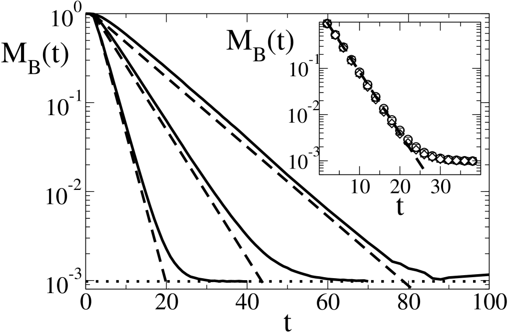
Figure 1: Main plot: Boltzmann echo for $N=1024$, $K_{1}=K_{2}=10.09$, and $\sigma_{1}=0.0018$ ($\Gamma_{\Sigma_{1}}\simeq 0.09$). Data have been calculated from 50 different initial states. The full lines correspond to $\epsilon=0$, 0.0018 and 0.0037 (from right to left) and the dashed lines give the predicted exponential decay of Eq. (4), with $\Gamma_{\cal U}=1.2\,10^{4}\epsilon^{2},\Gamma_{\Sigma_{1}}=2.6\,10^{4}\sigma_{1}^{2}$, $\lambda=1.6\gg\Gamma_{\cal U},\Gamma_{\Sigma_{1}}$ (dashed lines have been slightly shifted for clarity). The dotted line gives the saturation $N^{-1}.\,$ Inset : ${\cal M}_{\rm B}$ for $\epsilon=0.0037$, and $\sigma_{1}=0.0003$ (circles; $\Gamma_{\Sigma_{1}}\simeq 2.\,10^{-3}$), $\sigma_{1}=0.0006$ (squares; $\Gamma_{\Sigma_{1}}\simeq 9.\,10^{3}$), and $0.0009$ (diamonds; $\Gamma_{\Sigma_{1}}\simeq 0.02$). The dashed line indicates the theoretical prediction ${\cal M}_{\rm B}(t)=\exp[-0.3t]$.

We numerically illustrate our findings. We consider two coupled kicked rotators with Hamiltonian

$$H_{i} = p_{i}^{2}/2+K_{i}\cos(x_{i})\;\sum_{n}\delta(t-nT),$$ (15a)

$${\cal U} = \epsilon\;\sin(x_{1}-x_{2}-0.33)\;\sum_{n}\delta(t-nT).$$ (15b)

We concentrate on the regime $K_{i}>7$, for which the dynamics is fully chaotic with Lyapunov exponent $\lambda_{i}\approx\ln[K_{i}/2]$. The time-reversed one-particle Hamiltonians are obtained through $K_{i}\rightarrow K_{i}+\sigma_{i}$. We here restrict ourselves to the case ${\cal U}={\cal U}_{\rm f}={\cal U}_{\rm b}$. Both rotators are quantized on the torus with discrete momenta $p_{n}=2\pi n/N$, $n=1,2,...N$. The one- and two-particle bandwidths and level spacings are given by $B_{1}=2\pi$, $\delta_{1}=2\pi/N$ and $B_{2}=4\pi$, $\delta_{2}=4\pi/N^{2}$. For more details on the numerical procedure, we refer the reader to Ref. Izr .

We first checked that ${\cal M}_{\rm B}(t)$ is independent of $K_{2}$ (as long as system 2 remains chaotic) and $\sigma_{2}$, and therefore set $K_{2}=K_{1}$, $\sigma_{2}=0$. The main panel in Fig. 1 shows that for $B_{1}>\Gamma_{\Sigma_{1}}>\delta_{1}$, $B_{2}>\Gamma_{\cal U}>\delta_{2}$, Eq. (4) is satisfied. Additionally, the inset of Fig. 1 illustrates that when $\Gamma_{\Sigma_{1}}\ll 2\Gamma_{\cal U}$, the observed decay is only sensitive to ${\cal U}$ , and one effectively obtains a $\Sigma_{1}$-independent decay. Further unshown data confirm the existence of the Lyapunov decay [second term in Eq. (4)]. All our numerical results thus confirm the validity of Eq. (4).

In conclusion we propose to analyze echo experiments in the light of the Boltzmann echo of Eq. (2) and (3). Our semiclassical and RMT analysis showed that the decay of ${\cal M}_{\rm B}(t)$ saturates at a finite value even when the time-reversal operation is performed with infinite accuracy. Further work should attempt to connect these results with echo experiments nmr ; kurnit ; davidson ; nakamura ; levstein .

One of us (CP) acknowledges the support of the Swiss National Science Foundation.

References

• (1) J. Loschmidt, J. Sitzungsber. der kais. Akad. d. W. Math. Naturw. II 73, 128 (1876).
• (2) For references on Maxwell’s, Gibbs’ and Boltzmann’s probabilistic interpretation of the second law and a discussion of the microscopic origin of macroscopic irreversibility see e.g.: J.L. Lebowitz, Physica A 263, 516 (1999).
• (3) L. Boltzmann, Ann. der Phys. 57, 773 (1896).
• (4) D.L. Shepelyansky, Physica D 8, 208 (1983).
• (5) A. Peres, Phys. Rev. A 30, 1610 (1984).
• (6) R.A. Jalabert and H.M. Pastawski, Phys. Rev. Lett. 86, 2490 (2001).
• (7) E.L. Hahn, Phys. Rev. 80, 580 (1950).
• (8) S. Zhang, B.H. Meier, and R.R. Ernst, Phys. Rev. Lett. 69, 2149 (1992); H.M. Pastawski, P. R. Levstein, G. Usaj, Phys. Rev. Lett. 75, 4310 (1995).
• (9) N.A. Kurnit, I.D. Abella, and S.R. Hartmann, Phys. Rev. Lett. 13, 567 (1964).
• (10) F.B.J. Buchkremer, R. Dumke, H. Levsen, G. Birkl, and W. Ertmer, Phys. Rev. Lett. 85, 3121 (2000); M.F Andersen, A. Kaplan, and N. Davidson, Phys. Rev. Lett. 90, 023001 (2003).
• (11) Y. Nakamura, Yu.A. Pashkin, T. Yamamoto, and J.S. Tsai, Phys. Rev. Lett. 88, 047901 (2002).
• (12) Ph. Jacquod, P.G. Silvestrov, and C.W.J. Beenakker, Phys. Rev. E 64, 055203(R) (2001).
• (13) Ph. Jacquod, Phys. Rev. Lett. 92, 150403 (2004); ibid 93, 219903 (2004).
• (14) C. Petitjean and Ph. Jacquod, quant-ph/0510157.
• (15) H.M. Pastawski, P.R. Levstein, G. Usaj, J. Raya, and J. Hirschinger, Physica A 283, 166 (2000).
• (16) P. Cvitanović, R. Artuso, R. Mainieri, G. Tanner, and G. Vattay, Chaos: Classical and Quantum, ChaosBook.org (Niels Bohr Institute, Copenhagen 2003).
• (17) This is rigorously justified by the structural stability of hyperbolic systems considered here; see e.g. J. Vanicek and E.J. Heller, Phys. Rev. E 68, 056208 (2003).
• (18) F.M. Izrailev, Phys. Rep. 196, 334 (1979).