Properties of entangled photon pairs generated in one-dimensional nonlinear photonic-band-gap structures

Abstract

We have developed a rigorous quantum model of spontaneous parametric down-conversion in a nonlinear 1D photonic-band-gap structure based upon expansion of the field into monochromatic plane waves. The model provides a two-photon amplitude of a created photon pair. The spectra of the signal and idler fields, their intensity profiles in the time domain, as well as the coincidence-count interference pattern in a Hong-Ou-Mandel interferometer are determined both for cw and pulsed pumping regimes in terms of the two-photon amplitude. A broad range of parameters characterizing the emitted down-converted fields can be used. As an example, a structure composed of 49 layers of GaN/AlN is analyzed as a suitable source of photon pairs having high efficiency.

I Introduction

More than 20 years ago, Hong, Ou, and Mandel showed experimentally that mutually strongly quantum correlated (entangled) photon pairs can be emitted in the nonlinear process of parametric down-conversion Hong1987 ; Mandel1995 at the single-photon level. For the occurrence of entangled photon pairs, the spontaneous character of the process is important. Entanglement of two photons comprising a photon pair might occur for various physical quantities like frequencies, emission angles (wave-vectors), or polarizations. Perhaps most interestingly, entangled photon pairs manifest themselves in time domain, where both photons are detected within a relatively narrow time window. This is a direct consequence of the ‘point’ character of the emission of a photon pair in the time domain. The width of the time window characterized by an entanglement time is typically on the order of several hundreds of fs, and is experimentally observable using Hong-Ou-Mandel interferometer.

In the time that has intervened since the original predictions, entangled photon pairs have been used for numerous experiments demonstrating both fundamental aspects of their physical properties Perina1994 and their potential for applications. These also include tests of Bell inequalities Perina1994 , quantum teleportation Bouwmeester1997 , the generation of Greenberger-Horne-Zeilinger states Bouwmeester1999 or quantum computation Bouwmeester2000 that can exploit photon pairs. Quantum cryptography with photon pairs Lutkenhaus2000 may be considered the most important application. We mention that applications to metrology have also been suggested Migdal1999 .

Most researchers in the field have focused their attention for the most part on bulk nonlinear crystals, pumped by intense laser beams in type I and type II configurations. Bright sources of polarization-entangled photon pairs have been fabricated using two nonlinear type I crystals, mutually rotated by 90 degrees Kwiat1999 ; Kwiat2001 ; Nambu2002 . The nonlinear processes in an optical cavity have also been used to enhance the photon-pair generation rate Shapiro2000 . In addition, periodically-poled materials may be used to increase the photon-pair generation rate in materials where phase matching is not naturally available Kuklewicz2005 . At present, even sources of photon pairs pumped by laser diodes have been developed Trojek2004 .

On the fabrication front, techniques of structures composed of nonlinear thin layers (of width of several tens or hundreds of nm) have developed to the point that useful structures with pre-defined properties may be achieved rather easily Bertolotti2001 . These nonlinear photonic-band-gap structures Yablonovitch1987 ; John1987 ; Joannopoulos1995 ; Sakoda2005 are very promising as sources of photon pairs, as has recently been shown in Vamivakas2004 ; Centini2005 . Despite the small amount of nonlinear material embedded inside them, they can generate photon pairs with relatively high efficiency thanks to the constructive interference that involves both the pump and the down-converted fields, their spatial inhomogeneity nothwithstanding. The enhancement of the photon-pair generation rate has been predicted to be several hundreds and even thousands of times larger than photon-pair generation rates in nonlinear, bulk materials Centini2005 . Moreover, the spectral and spatial characteristics of the down-converted fields depend on details of the structure, a fact that might be used to control the process, at least to some extent. For example, photon pairs with very narrow spectra may be obtained from suitable structures. We note that along the same vein, four-wave mixing in photonic-band-gap nonlinear fibers is also promising as a modern source of photon pairs Li2005 ; Fulconis2005 .

In this paper, we present a quantum model of photon-pair emission in a nonlinear, one-dimensional photonic-band-gap structure, based upon a perturbative solution of the Schrödinger equation. This model extends those developed for bulk nonlinear materials in Keller1997 ; Perinajr1999 ; DiGiuseppe1997 ; Grice1998 . It has been shown in Centini2005 that this approach is compatible with models based on methods of classical nonlinear optics (multiple-scale spatial and temporal expansion methods) with a specific kind of stochastic averaging concerning emitted spectra. The quantum model, however, provides a complete description of the nonlinear process.

The paper is organized as follows. In Sec. II, the model is presented in three steps. Description of a quantum field in a layered medium in Subsec. IIA is followed by the description of nonlinear quantum interactions in Subsec. IIB. In Subsec. IIC measurable characteristics of the generated down-converted fields are determined. The behavior of physical quantities characterizing a photon pair are discussed in Sec. III, both for cw and pulsed pumping regimes. Sec. IV contains our conclusions.

II Description of spontaneous parametric down-conversion in a one-dimensional, nonlinear photonic-band-gap structure

We consider a stack of $N$ nonlinear layers in which spontaneous parametric down-conversion may occur. A sketch of the system is shown in Fig. 1. The $l$th layer begins at $z=z_{l-1}$ and ends at $z=z_{l}$, its length is denoted as $L_{l}$, $l=1,\ldots,N$. Linear indices of refraction of pump, signal, and idler fields in the $l$th layer are denoted as $n_{p}^{(l)}$, $n_{s}^{(l)}$, and $n_{i}^{(l)}$, respectively. Symbols $n_{s}^{(0)}$, $n_{i}^{(0)}$, and $n_{p}^{(0)}$ ($n_{s}^{(N+1)}$, $n_{i}^{(N+1)}$, and $n_{p}^{(N+1)}$) mean indices of refraction in front of (beyond) the sample. The symbol $d^{(l)}$ is used for the nonlinear tensor of $l$th layer; symbols $k_{p}^{(l)}$, $k_{s}^{(l)}$, and $k_{i}^{(l)}$ stand for pump-, signal-, and idler- field wave-vectors in the $l$th layer.

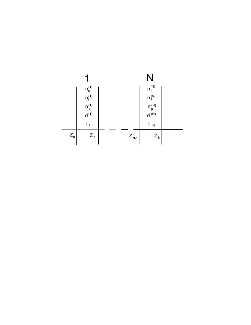
Figure 1: Scheme of the considered nonlinear one-dimensional layered structure: $n_{s}^{(l)}$, $n_{i}^{(l)}$, and $n_{p}^{(l)}$ denote indices of refraction of signal, idler, and pump fields in $l$th layer with the length $L_{l}$, $d^{(l)}$ stands for a nonlinear coefficient of $l$th layer and $z_{l}$ are positions of the boundaries.

II.1 Optical fields in a one-dimensional photonic-band-gap structure

The structure is pumped by a classical strong pump field that propagates under the angle $\vartheta_{p}$ with respect to $z$ axis (see Fig. 2). Its wave-vector ${\bf k}_{p}$ lyes in the $yz$ plane, whereas its electric-field amplitude ${\bf E}_{p_{F}}$ is perpendicular to the wave-vector ${\bf k}_{p}$.

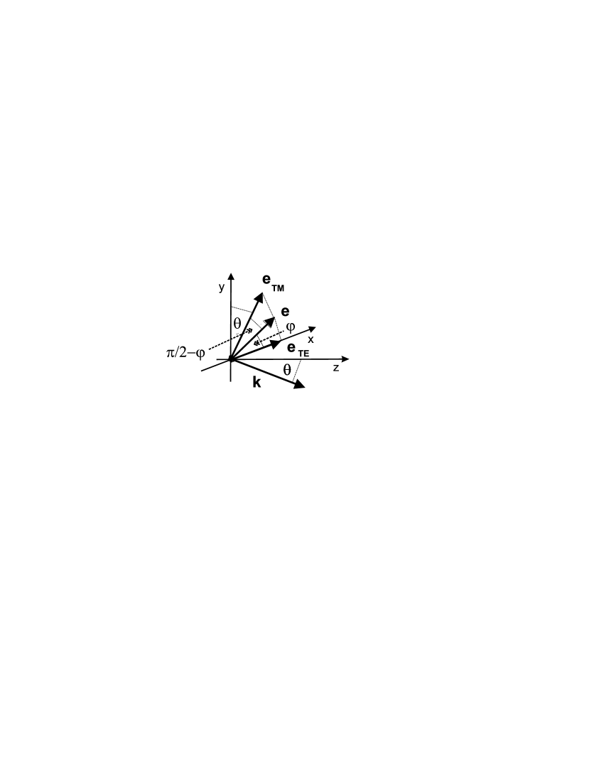
Figure 2: Scheme of the used coordinate system for the description of pump, signal, and idler fields. A field with wave-vector ${\bf k}$ (lying in $yz$ plane) and polarization vector ${\bf e}$ (perpendicular to ${\bf k}$) propagates at an angle $\vartheta$ with respect to $z$ axis. The field is linearly polarized and the polarization vector ${\bf e}$ makes an angle $\varphi$ with respect to $x$ axis. The polarization vector ${\bf e}_{TE}$ of TE wave is parallel to $x$ axis whereas the polarization vector ${\bf e}_{TM}$ of TM wave lyes in $yz$ plane.

The pump-field positive-frequency electric-field amplitude at the input of the structure at $z=z_{0}$ is denoted as ${\bf E}_{p_{F}}^{(+)}(z_{0},t)$ and can be conveniently described using a positive-frequency electric-field amplitude spectrum ${\bf E}_{p_{F}}^{(+)}(z_{0},\omega_{p})$ determined as follows:

$${\bf E}_{p_{F}}^{(+)}(z_{0},\omega_{p})=\frac{1}{\sqrt{2\pi}}\int_{-\infty}^{\infty}dt\,{\bf E}_{p_{F}}^{(+)}(z_{0},t)\exp(i\omega_{p}t).$$ (1)

If we assume a Gaussian time profile and a linear polarization of the incident electric-field amplitude ${\bf E}_{p_{F}}$ in the direction rotated by an angle $\varphi_{p}$ with respect to an incident TE-wave polarization direction ${\bf e}_{p_{F},TE}$ (${\bf e}_{p_{F},TM}$ denotes an incident TM-wave polarization direction, see Fig. 2) we have:

$${\bf E}_{p_{F}}^{(+)}(z_{0},t) = \left[{\bf e}_{p_{F},TE}\cos(\varphi_{p})+{\bf e}_{p_{F},TM}\sin(\varphi_{p})\right]$$ (2)

$$\mbox{}\times\xi_{p}\exp\left(-\frac{1+ia_{p}}{\tau_{p}^{2}}t^{2}\right)\exp(-i\omega_{p}^{0}t),$$

$$= {\bf E}_{p_{F},TE}^{(+)}(z_{0},t)+{\bf E}_{p_{F},TM}^{(+)}(z_{0},t),$$

where $\xi_{p}$ is the pump-pulse amplitude, $\tau_{p}$ pulse duration, $\omega_{p}^{0}$ central frequency, and $a_{p}$ denotes a chirp parameter of the pulse. The spectrum ${\bf E}_{p_{F}}^{(+)}(z_{0},\omega_{p})$ determined by Eq. (1) is given as:

$${\bf E}_{p_{F}}^{(+)}(z_{0},\omega_{p}) = \left[{\bf e}_{p_{F},TE}\cos(\varphi_{p})+{\bf e}_{p_{F},TM}\sin(\varphi_{p})\right]$$ (3)

$$\mbox{}\times\xi_{p}\frac{\tau_{p}}{\sqrt{2(1+ia_{p})}}\exp\left(-\frac{\tau_{p}^{2}}{4(1+ia_{p})}(\omega_{p}-\omega_{p}^{0})^{2}\right)$$

$$= {\bf E}_{p_{F},TE}^{(+)}(z_{0},\omega_{p})+{\bf E}_{p_{F},TM}^{(+)}(z_{0},\omega_{p}).$$

On the other hand, the following spectrum corresponds to cw pumping:

$${\bf E}_{p_{F}}^{(+)}(z_{0},\omega_{p}) = \left[{\bf e}_{p_{F},TE}\cos(\varphi_{p})+{\bf e}_{p_{F},TM}\sin(\varphi_{p})\right]$$ (4)

$$\mbox{}\times\xi_{p}\delta(\omega_{p}-\omega_{p}^{0});$$

$\delta$ means a Dirac delta function.

The pump field incident on the structure is scattered at each boundary inside the structure, so as to achieve a certain profile along the $z$ axis, provided that the nonlinear interaction does not lead to pump-field depletion. Scattering of the pump field is conveniently described using its decomposition into monochromatic waves. The positive-frequency electric-field amplitude ${\bf E}_{p,\alpha}^{(+)}(z,\omega_{p})$ of a monochromatic component at frequency $\omega_{p}$ with polarization $\alpha$ ($\alpha=$ TE, TM) can be written as follows Yeh1988 :

$${\bf E}_{p,\alpha}^{(+)}(z,\omega_{p}) = {\rm rect}_{-\infty,z_{0}}(z)$$ (5)

$$\mbox{}\times\left[A_{p_{F},\alpha}^{(0)}(\omega_{p}){\bf e}_{p_{F},\alpha}^{(0)}(\omega_{p})\exp(i{\bf k}_{p,z}^{(0)}(z-z_{0}))\right.$$

$$\mbox{}\left.+A_{p_{B},\alpha}^{(0)}(\omega_{p}){\bf e}_{p_{B},\alpha}^{(0)}(\omega_{p})\exp(-i{\bf k}_{p,z}^{(0)}(z-z_{0}))\right]$$

$$\mbox{}+\sum_{l=1}^{N}{\rm rect}_{z_{l-1},z_{l}}(z)$$

$$\mbox{}\times\left[A_{p_{F},\alpha}^{(l)}(\omega_{p}){\bf e}_{p_{F},\alpha}^{(l)}(\omega_{p})\exp(i{\bf k}_{p,z}^{(l)}(z-z_{l-1}))\right.$$

$$\mbox{}\left.+A_{p_{B},\alpha}^{(l)}(\omega_{p}){\bf e}_{p_{B},\alpha}^{(l)}(\omega_{p})\exp(-i{\bf k}_{p,z}^{(l)}(z-z_{l-1}))\right]$$

$$\mbox{}+{\rm rect}_{z_{N},\infty}(z)$$

$$\mbox{}\times\left[A_{p_{F},\alpha}^{(N+1)}(\omega_{p}){\bf e}_{p_{F},\alpha}^{(N+1)}(\omega_{p})\exp(i{\bf k}_{p,z}^{(N+1)}(z-z_{N}))\right.$$

$$\mbox{}\left.+A_{p_{B},\alpha}^{(N+1)}(\omega_{p}){\bf e}_{p_{B},\alpha}^{(N+1)}(\omega_{p})\exp(-i{\bf k}_{p,z}^{(N+1)}(z-z_{N}))\right];$$

$$\alpha=TE,TM;$$

the function ${\rm rect}_{z_{a},z_{b}}(z)$ equals one for $z_{a}\leq z\leq z_{b}$ and is zero otherwise. Polarization vectors of $\alpha$-waves in $l$th layer are denoted as ${\bf e}^{(l)}_{p_{F},\alpha}$ and ${\bf e}^{(l)}_{p_{B},\alpha}$ for forward- and backward-propagating fields with respect to $z$ axis, respectively, and they are frequency dependent. The symbol ${\bf k}_{p,z}^{(l)}$ denotes a $z$ component of the pump-field wave-vector ${\bf k}_{p}^{(l)}$ in $l$th layer and is determined by the expression

$${\bf k}_{p,z}^{(l)}={\bf k}_{p}^{(l)}\cos(\vartheta_{p}^{(l)}),$$ (6)

where the wave-vector ${\bf k}_{p}^{(l)}$ propagates in the $l$th layer under the angle $\vartheta_{p}^{(l)}$ with respect to $z$ axis. The angles $\vartheta_{p}^{(l)}$ fulfill the Snell law at the boundaries, i.e.

$$n_{p}^{(l)}\sin(\vartheta_{p}^{(l)})=n_{p}^{(l+1)}\sin(\vartheta_{p}^{(l+1)}),\hskip 14.22636ptl=0,\ldots,N;$$ (7)

$\vartheta_{p}^{(0)}=\vartheta_{p}$.

The symbol $A_{p_{F},\alpha}^{(0)}(\omega_{p})$ is identified as an electric-field amplitude of the pump field at frequency $\omega_{p}$ with polarization $\alpha$ incident on the structure from the left-hand side, whereas the symbol $A_{p_{B},\alpha}^{(N+1)}(\omega_{p})$ describes an electric-field amplitude of the pump field at frequency $\omega_{p}$ with polarization $\alpha$ incident from the right-hand side. The remaining amplitudes $A_{p_{F},\alpha}^{(l)}(\omega_{p})$ and $A_{p_{B},\alpha}^{(l)}(\omega_{p})$ are determined using relations at the boundaries and free-field propagation inside the layers:

$$\pmatrix{A_{p_{F},\alpha}^{(1)}(\omega_{p})\cr A_{p_{B},\alpha}^{(1)}(\omega_{p})} = {\cal T}_{p,\alpha}^{(0)}(\omega_{p})\pmatrix{A_{p_{F},\alpha}^{(0)}(\omega_{p})\cr A_{p_{B},\alpha}^{(0)}(\omega_{p})},$$

$$\pmatrix{A_{p_{F},\alpha}^{(l+1)}(\omega_{p})\cr A_{p_{B},\alpha}^{(l+1)}(\omega_{p})} = {\cal T}_{p,\alpha}^{(l)}(\omega_{p}){\cal P}_{p}^{(l)}(\omega_{p})\pmatrix{A_{p_{F},\alpha}^{(l)}(\omega_{p})\cr A_{p_{B},\alpha}^{(l)}(\omega_{p})},$$ (8)

$$\alpha=TE,TM;\;\;l=1,\ldots,N.$$

We note that the coefficients $A_{p_{F},\alpha}^{(l)}$ and $A_{p_{B},\alpha}^{(l)}$ for $l=1,\ldots,N$ describe the corresponding electric-field amplitudes at the beginning of $l$th layer.

Assuming TE and TM waves, the boundary transfer matrices ${\cal T}_{p,TE}^{(l)}$ and ${\cal T}_{p,TM}^{(l)}$ have the form:

$${\cal T}_{p,TE}^{(l)}(\omega_{p}) =$$

$$\frac{1}{2}\pmatrix{1+f^{(l)}_{p}(\omega_{p})g^{(l)}_{p}(\omega_{p})&1-f^{(l)}_{p}(\omega_{p})g^{(l)}_{p}(\omega_{p})\cr 1-f^{(l)}_{p}(\omega_{p})g^{(l)}_{p}(\omega_{p})&1+f^{(l)}_{p}(\omega_{p})g^{(l)}_{p}(\omega_{p})},$$

$${\cal T}_{p,TM}^{(l)}(\omega_{p}) =$$ (9)

$$\frac{1}{2}\pmatrix{f^{(l)}_{p}(\omega_{p})+g^{(l)}_{p}(\omega_{p})&f^{(l)}_{p}(\omega_{p})-g^{(l)}_{p}(\omega_{p})\cr f^{(l)}_{p}(\omega_{p})-g^{(l)}_{p}(\omega_{p})&f^{(l)}_{p}(\omega_{p})+g^{(l)}_{p}(\omega_{p})},$$

$$\;\;l=0,\ldots,N;$$

$f^{(l)}_{p}=\cos(\vartheta_{p}^{(l)})/\cos(\vartheta_{p}^{(l+1)})$ and $g^{(l)}_{p}=n_{p}^{(l)}/n_{p}^{(l+1)}$. The free-field propagation matrices ${\cal P}_{p}^{(l)}(\omega_{p})$ can be written as:

$${\cal P}_{p}^{(l)}(\omega_{p}) = \pmatrix{\exp(i{\bf k}_{p,z}^{(l)}L_{l})&0\cr 0&\exp(-i{\bf k}_{p,z}^{(l)}L_{l})},$$ (10)

$$l=1,\ldots,N.$$

The positive-frequency electric-field operators $\hat{\bf E}_{s}^{(+)}(z,t)$ and $\hat{\bf E}_{i}^{(+)}(z,t)$ for the signal and idler fields can be decomposed into TE- and TM-wave contributions $\hat{\bf E}_{s,TE}^{(+)}(z,t)$, $\hat{\bf E}_{s,TM}^{(+)}(z,t)$, $\hat{\bf E}_{i,TE}^{(+)}(z,t)$, and $\hat{\bf E}_{i,TM}^{(+)}(z,t)$ and expressed as follows Vogel2001 :

$$\hat{\bf E}_{m}^{(+)}(z,t) = \sum_{\alpha=TE,TM}\int_{0}^{\infty}d\omega_{m}\sqrt{\frac{\hbar\omega_{m}}{4\pi\epsilon_{0}c{\cal B}}}$$ (11)

$$\mbox{}\times\left[\hat{a}_{m_{F},\alpha}(z,\omega_{m}){\bf e}_{m_{F},\alpha}(z,\omega_{m})\right.$$

$$\mbox{}\left.+\hat{a}_{m_{B},\alpha}(z,\omega_{m}){\bf e}_{m_{B},\alpha}(z,\omega_{m})\right]\exp(-i\omega_{m}t)$$

$$=\hat{\bf E}_{m,TE}^{(+)}(z,t)+\hat{\bf E}_{m,TM}^{(+)}(z,t)$$

$$=\frac{1}{\sqrt{2\pi}}\int_{0}^{\infty}d\omega_{m}\hat{\bf E}_{m}^{(+)}(z,\omega_{m})$$

$$=\frac{1}{\sqrt{2\pi}}\int_{0}^{\infty}d\omega_{m}\left[\hat{\bf E}_{m,TE}^{(+)}(z,\omega_{m})+\hat{\bf E}_{m,TM}^{(+)}(z,\omega_{m})\right],$$

$$m=s,i.$$

The permittivity of vacuum is denoted as $\epsilon_{0}$; $c$ means speed of light in vacuum, $\hbar$ is the reduced Planck constant, and $\cal B$ denotes the area of the transverse profile of a beam. The symbols ${\bf e}_{m_{F},\alpha}(z,\omega_{m})$ and ${\bf e}_{m_{B},\alpha}(z,\omega_{m})$ mean polarization vectors of mode $m$ of $\alpha$ wave propagating forward and backward with respect to the $z$ axis. Annihilation operators of signal [$\hat{a}_{s_{F},\alpha}(z,\omega_{s})$, $\hat{a}_{s_{B},\alpha}(z,\omega_{s})$] and idler [$\hat{a}_{i_{F},\alpha}(z,\omega_{i})$, $\hat{a}_{i_{B},\alpha}(z,\omega_{i})$] photons in $\alpha$ wave introduced in Eq. (11) can be expressed in the same way as the pump-field amplitude ${\bf E}_{p,\alpha}^{(+)}(z,\omega_{p})$:

$$\hat{a}_{m_{F},\alpha}(z,\omega_{m}){\bf e}_{m_{F},\alpha}(z,\omega_{m})+\hat{a}_{m_{B},\alpha}(z,\omega_{m}){\bf e}_{m_{B},\alpha}(z,\omega_{m})$$ (12)

$$={\rm rect}_{-\infty,z_{0}}(z)$$

$$\mbox{}\times\left[\hat{a}_{m_{F},\alpha}^{(0)}(\omega_{m}){\bf e}_{m_{F},\alpha}^{(0)}(\omega_{m})\exp(i{\bf k}_{m,z}^{(0)}(z-z_{0}))\right.$$

$$\mbox{}\left.+\hat{a}_{m_{B},\alpha}^{(0)}(\omega_{m}){\bf e}_{m_{B},\alpha}^{(0)}(\omega_{m})\exp(-i{\bf k}_{m,z}^{(0)}(z-z_{0}))\right]$$

$$\mbox{}+\sum_{l=1}^{N}{\rm rect}_{z_{l-1},z_{l}}(z)$$

$$\mbox{}\times\left[\hat{a}_{m_{F},\alpha}^{(l)}(\omega_{m}){\bf e}_{m_{F},\alpha}^{(l)}(\omega_{m})\exp(i{\bf k}_{m,z}^{(l)}(z-z_{l-1}))\right.$$

$$\mbox{}\left.+\hat{a}_{m_{B},\alpha}^{(l)}(\omega_{m}){\bf e}_{m_{B},\alpha}^{(l)}(\omega_{m})\exp(-i{\bf k}_{m,z}^{(l)}(z-z_{l-1}))\right]$$

$$\mbox{}+{\rm rect}_{z_{N},\infty}(z)$$

$$\mbox{}\times\left[\hat{a}_{m_{F},\alpha}^{(N+1)}(\omega_{m}){\bf e}_{m_{F},\alpha}^{(N+1)}(\omega_{m})\exp(i{\bf k}_{m,z}^{(N+1)}(z-z_{N}))\right.$$

$$\mbox{}\left.+\hat{a}_{m_{B},\alpha}^{(N+1)}(\omega_{m}){\bf e}_{m_{B},\alpha}^{(N+1)}(\omega_{m})\exp(-i{\bf k}_{m,z}^{(N+1)}(z-z_{N}))\right],$$

$$m=s,i;\;\;\alpha=TE,TM.$$

The polarization vectors ${\bf e}_{m_{F},\alpha}^{(l)}$ and ${\bf e}_{m_{B},\alpha}^{(l)}$ give the polarization directions of mode $m$ with $\alpha$ wave in $l$th layer propagating forward and backward, respectively, whereas ${\bf k}_{m,z}^{(l)}$ is a $z$ component of the wave vector ${\bf k}_{m}^{(l)}$ of this mode:

$${\bf k}_{m,z}^{(l)}={\bf k}_{m}^{(l)}\cos(\vartheta_{m}^{(l)}),\hskip 14.22636ptm=s,i.$$ (13)

The angle $\vartheta_{m}^{(l)}$ characterizes the direction of propagation of mode $m$ with respect to the $z$ axis. The angles $\vartheta_{m}^{(l)}$ are given by the Snell law at the boundaries, i.e.

$$n_{m}^{(l)}\sin(\vartheta_{m}^{(l)}) = n_{m}^{(l+1)}\sin(\vartheta_{m}^{(l+1)}),$$ (14)

$$m=s,i;\;\;l=0,\ldots,N;$$

$\vartheta_{m}^{(0)}=\vartheta_{m}$, where $\vartheta_{m}$ stands for the angle of incidence of mode $m$.

The operators $\hat{a}_{m_{F},\alpha}^{(l)}(\omega_{m})$ and $\hat{a}_{m_{B},\alpha}^{(l)}(\omega_{m})$ obey the following commutation relations:

$$[\hat{a}_{m_{F},\alpha}^{(l)}(\omega_{m}),\hat{a}_{m^{\prime}_{F},\alpha^{\prime}}^{(l^{\prime})\dagger}(\omega^{\prime}_{m})] = \delta_{\alpha,\alpha^{\prime}}\delta_{m,m^{\prime}}\delta_{l,l^{\prime}}\delta(\omega_{m}-\omega^{\prime}_{m}),$$

$${}[\hat{a}_{m_{F},\alpha}^{(l)}(\omega_{m}),\hat{a}_{m^{\prime}_{F},\alpha^{\prime}}^{(l^{\prime})}(\omega^{\prime}_{m})] = 0,$$

$${}[\hat{a}_{m_{B},\alpha}^{(l)}(\omega_{m}),\hat{a}_{m^{\prime}_{B},\alpha^{\prime}}^{(l^{\prime})\dagger}(\omega^{\prime}_{m})] = \delta_{\alpha,\alpha^{\prime}}\delta_{m,m^{\prime}}\delta_{l,l^{\prime}}\delta(\omega_{m}-\omega^{\prime}_{m}),$$

$${}[\hat{a}_{m_{B},\alpha}^{(l)}(\omega_{m}),\hat{a}_{m^{\prime}_{B},\alpha^{\prime}}^{(l^{\prime})}(\omega^{\prime}_{m})] = 0,$$

$${}[\hat{a}_{m_{F},\alpha}^{(l)}(\omega_{m}),\hat{a}_{m^{\prime}_{B},\alpha^{\prime}}^{(l^{\prime})}(\omega^{\prime}_{m})] = 0,$$

$${}[\hat{a}_{m_{F},\alpha}^{(l)}(\omega_{m}),\hat{a}_{m^{\prime}_{B},\alpha^{\prime}}^{(l^{\prime})\dagger}(\omega^{\prime}_{m})] = 0;$$ (15)

$$m,m^{\prime}=s,i;\;\;\alpha=TE,TM;\;\;l,l^{\prime}=0,\ldots,N+1.$$

The photonic-band-gap structure imposes the following relations among the operators $\hat{a}_{m_{F},\alpha}^{(l)}(\omega_{m})$ and $\hat{a}_{m_{B},\alpha}^{(l)}(\omega_{m})$ acting in $l$th layer:

$$\pmatrix{\hat{a}_{m_{F},\alpha}^{(1)}(\omega_{m})\cr\hat{a}_{m_{B},\alpha}^{(1)}(\omega_{m})} = {\cal T}_{m,\alpha}^{(0)}(\omega_{m})\pmatrix{\hat{a}_{m_{F},\alpha}^{(0)}(\omega_{m})\cr\hat{a}_{m_{B},\alpha}^{(0)}(\omega_{m})},$$

$$\pmatrix{\hat{a}_{m_{F},\alpha}^{(l+1)}(\omega_{m})\cr\hat{a}_{m_{B},\alpha}^{(l+1)}(\omega_{m})} = {\cal T}_{m,\alpha}^{(l)}{\cal P}_{m}^{(l)}\pmatrix{\hat{a}_{m_{F},\alpha}^{(l)}(\omega_{m})\cr\hat{a}_{m_{B},\alpha}^{(l)}(\omega_{m})},$$ (16)

$$m=s,i;\;\;\alpha=TE,TM;\;\;l=1,\ldots,N.$$

Transfer matrices ${\cal T}^{(l)}_{m,\alpha}$ at the boundaries and free-field propagation matrices ${\cal P}^{(l)}_{m}$ for $m=s,i$ and $\alpha=TE,TM$ are defined in the same way as those given in Eqs. (9) and (10) for the pump-field amplitudes.

II.2 Nonlinear interaction inside the photonic-band-gap structure

The Hamiltonian $\hat{H}(t)$ describing spontaneous parametric down-conversion in a nonlinear medium of volume $\cal V$ at time $t$ can be written as:

$$\hat{H}(t) = \epsilon_{0}\int_{\cal V}d{\bf r}\;$$ (17)

$${\bf d}({\bf r}):\left[{\bf E}_{p}^{(+)}({\bf r},t)\hat{\bf E}_{s}^{(-)}({\bf r},t)\hat{\bf E}_{i}^{(-)}({\bf r},t)+{\rm h.c.}\right],$$

where ${\bf d}$ denotes a third-order tensor of nonlinear coefficients, the symbol $:$ is shorthand of the tensor ${\bf d}$ with respect to its three indices, and ${\rm h.c.}$ stands for a hermitian conjugated term. The negative-frequency electric-field operators $\hat{\bf E}_{m}^{(-)}$ for $m=s,i$ have been introduced in Eq. (17) ($\hat{\bf E}_{m}^{(-)}=\hat{\bf E}_{m}^{(+)\dagger}$). Decomposing the interacting fields into TE and TM waves, and using the inverse Fourier transformation in Eq. (17), we arrive at:

$$\hat{H}(t) = \frac{\epsilon_{0}{\cal B}}{\sqrt{2\pi}}\int_{0}^{L}dz\int_{0}^{\infty}d\omega_{p}\int_{0}^{\infty}d\omega_{s}\int_{0}^{\infty}d\omega_{i}$$ (18)

$$\sum_{\alpha,\beta,\gamma=TE,TM}{\bf d}(z):\Bigl{[}{\bf E}_{p,\alpha}^{(+)}(z,\omega_{p})\hat{\bf E}_{s,\beta}^{(-)}(z,\omega_{s})\hat{\bf E}_{i,\gamma}^{(-)}(z,\omega_{i})$$

$$+{\rm h.c.}\Bigr{]}.$$

Integrations over the variables $x$ and $y$ in Eq. (17) impose conditions for $x$ and $y$ component of wave-vectors; $\delta({\bf k}_{s,x}+{\bf k}_{i,x})$ [${\bf k}_{p,x}=0$ is assumed] and $\delta({\bf k}_{s,y}+{\bf k}_{i,y}-{\bf k}_{p,y})$. The latter $\delta$-function provides the following relation between the angles $\vartheta_{s}^{(l)}$ and $\vartheta_{i}^{(l)}$ of modes $s$ and $i$ in the $l$th layer:

$$\vartheta_{i}^{(l)} = \arcsin\left[\frac{\omega_{p}}{\omega_{i}}\sin(\vartheta_{p}^{(l)})-\frac{\omega_{s}}{\omega_{i}}\sin(\vartheta_{s}^{(l)})\right],$$ (19)

$$l=0,\ldots,N+1.$$

Solution of the Schrödinger equation to first order in nonlinear perturbation together with the assumption of incident vacuum state $|{\rm vac}\rangle$ in signal and idler fields provides the output state $|\psi\rangle_{s,\beta,i,\gamma}^{\rm out}$ of signal field with $\beta$ polarization and idler field with $\gamma$ polarization in the form:

$$|\psi\rangle_{s,\beta,i,\gamma}^{\rm out} = |{\rm vac}\rangle-\frac{i}{2\sqrt{2\pi}c}\sum_{l=1}^{N}\int_{0}^{\infty}\,d\omega_{p}\int_{0}^{\infty}\,d\omega_{s}\sqrt{\omega_{s}}$$ (20)

$$\mbox{}\times\int_{0}^{\infty}\,d\omega_{i}\sqrt{\omega_{i}}\sum_{l=1}^{N}\sum_{m=p_{F},p_{B}}\sum_{n=s_{F},s_{B}}\sum_{o=i_{F},i_{B}}$$

$$\mbox{}\times\sum_{\alpha=TE,TM}{\bf d}^{(l)}:{\bf e}_{m,\alpha}^{(l)}(\omega_{p}){\bf e}_{n,\beta}^{(l)}(\omega_{s}){\bf e}_{o,\gamma}^{(l)}(\omega_{i})$$

$$\mbox{}\times A_{m,\alpha}^{(l)}(\omega_{p})L_{l}\exp\left[+\frac{i}{2}(K_{m}^{(l)}-K_{n}^{(l)}-K_{o}^{(l)})L_{l}\right]$$

$$\mbox{}\times{\rm sinc}\left[\frac{1}{2}(K_{m}^{(l)}-K_{n}^{(l)}-K_{o}^{(l)})L_{l}\right]\delta(\omega_{p}-\omega_{s}-\omega_{i})$$

$$\mbox{}\times\hat{a}_{n,\beta}^{(l)\dagger}(\omega_{s})\hat{a}_{o,\gamma}^{(l)\dagger}(\omega_{i})|{\rm vac}\rangle.$$

The wave-vectors $K^{(l)}$ introduced in Eq. (20) are defined as $K_{j_{F}}^{(l)}={\bf k}_{j,z}^{(l)}$ and $K_{j_{B}}^{(l)}=-{\bf k}_{j,z}^{(l)}$ for $j=p,s,i$.

The operators $\hat{a}_{m_{F},\alpha}^{(l)}$ and $\hat{a}_{m_{B},\alpha}^{(l)}$ for $\alpha$ waves in mode $m$ in $l$th layer can be expressed in terms of the operators $\hat{a}_{m_{F},\alpha}^{(N+1)}$ and $\hat{a}_{m_{B},\alpha}^{(0)}$. These relations can be, e.g., written in the form:

$$\pmatrix{\hat{a}_{m_{F},\alpha}^{(l)}(\omega_{m})\cr\hat{a}_{m_{B},\alpha}^{(l)}(\omega_{m})} = \prod_{j=l}^{1}\left[{\cal P}_{m}^{(j)}(\omega_{m}){\cal T}_{m,\alpha}^{(j-1)}(\omega_{m})\right]$$ (21)

$$\mbox{}\times\pmatrix{1/({\cal S}_{m,\alpha})_{11}(\omega_{m})&-({\cal S}_{m,\alpha})_{12}(\omega_{m})/({\cal S}_{m,\alpha})_{11}(\omega_{m})\cr 0&1}$$

$$\mbox{}\times\pmatrix{\hat{a}_{m_{F},\alpha}^{(N+1)}(\omega_{m})\cr\hat{a}_{m_{B},\alpha}^{(0)}(\omega_{m})},$$

$$m=s,i;\;\;\alpha=TE,TM;\;\;l=1,\ldots,N.$$

The matrix ${\cal S}_{m,\alpha}$ used in Eq. (21) describes the propagation of $\alpha$ wave in field $m$ through the whole structure:

$${\cal S}_{m,\alpha}(\omega_{m}) = {\cal T}_{m,\alpha}^{(N)}(\omega_{m})\prod_{j=N}^{1}\left[{\cal P}_{m}^{(j)}(\omega_{m}){\cal T}_{m,\alpha}^{(j-1)}(\omega_{m})\right],$$ (22)

$$m=s,i;\;\;\alpha=TE,TM.$$

Similarly, the pump-field amplitudes $A_{p_{F},\alpha}^{(l)}$ and $A_{p_{B},\alpha}^{(l)}$ for $\alpha$ waves in $l$th layer can be determined from the amplitudes of the incident fields $A_{p_{F},\alpha}^{(0)}$ and $A_{p_{B},\alpha}^{(N+1)}$ as follows:

$$\pmatrix{A_{p_{F},\alpha}^{(l)}(\omega_{p})\cr A_{p_{B},\alpha}^{(l)}(\omega_{p})} = \prod_{j=l}^{1}\left[{\cal P}_{p}^{(j)}(\omega_{p}){\cal T}_{p,\alpha}^{(j-1)}(\omega_{p})\right]$$ (23)

$$\mbox{}\times\pmatrix{1&0\cr-({\cal S}_{p,\alpha})_{21}(\omega_{p})/({\cal S}_{p,\alpha})_{22}(\omega_{p})&1/({\cal S}_{p,\alpha})_{22}(\omega_{p})}$$

$$\mbox{}\times\pmatrix{A_{p_{F},\alpha}^{(0)}(\omega_{p})\cr A_{p_{B},\alpha}^{(N+1)}(\omega_{p})},$$

$$\alpha=TE,TM;\;\;l=1,\ldots,N.$$

The matrix ${\cal S}_{p,\alpha}$ describes the propagation of a classical pump field with polarization $\alpha$ through the whole structure, i.e.

$${\cal S}_{p,\alpha}(\omega_{p})={\cal T}_{p,\alpha}^{(N)}(\omega_{p})\prod_{j=N}^{1}\left[{\cal P}_{p}^{(j)}(\omega_{p}){\cal T}_{p,\alpha}^{(j-1)}(\omega_{p})\right].$$ (24)

We note that the expression in Eq. (20) for the output state $|\psi\rangle_{s,\beta,i,\gamma}^{\rm out}$ including relations written in Eqs. (21-24) can be formally recast into a compact form using the so-called left-to-right ($\Phi^{(+)}$) and right-to-left ($\Phi^{(-)}$) modes introduced in the classical electro-magnetic theory of layered structures (for details, see Centini2005 ). Fields exiting the structure at $z=z_{N}$ are described by $\Phi^{(+)}(z)$ functions, whereas $\Phi^{(-)}(z)$ functions are appropriate for fields exiting at $z=z_{0}$. In classical theory, this corresponds to the picture in which every nonlinear layer is a source (emitting ’dipole’) of photon pairs Aguanno2004 and the fields leaving the structure are given as a sum of contributions from all layers.

We assume that the outgoing signal (idler) field is detected using an analyzer with the polarization that forms an angle $\varphi_{s}$ ($\varphi_{i}$) with respect to the TE-wave polarization direction (see Fig. 2). In order to get the right wave-function, we transform the operators of the outgoing signal (idler) fields into the basis with the polarization vectors given by angles $\varphi_{s}$ ($\varphi_{i}$) and $\varphi_{s}+\pi/2$ ($\varphi_{i}+\pi/2$) using the following formulas:

$$\pmatrix{\hat{a}_{m_{F},TE}^{(N+1)}\cr\hat{a}_{m_{F},TM}^{(N+1)}} =$$

$$\pmatrix{\cos(\varphi_{m})&\sin(\varphi_{m})\cr-\sin(\varphi_{m})&\cos(\varphi_{m})}\pmatrix{\hat{a}_{m_{F},\varphi_{m}}^{(N+1)}\cr\hat{a}_{m_{F},\varphi_{m}+\pi/2}^{(N+1)}},$$

$$\pmatrix{\hat{a}_{m_{B},TE}^{(0)}\cr\hat{a}_{m_{B},TM}^{(0)}} =$$ (25)

$$\pmatrix{\cos(\varphi_{m})&\sin(\varphi_{m})\cr-\sin(\varphi_{m})&\cos(\varphi_{m})}\pmatrix{\hat{a}_{m_{B},\varphi_{m}}^{(0)}\cr\hat{a}_{m_{B},\varphi_{m}+\pi/2}^{(0)}},$$

$$m=s,i.$$

Substituting relations in Eqs. (21), (23), and (25) into the expression $|\psi\rangle_{s,TE,i,TE}^{\rm out}+|\psi\rangle_{s,TE,i,TM}^{\rm out}+|\psi\rangle_{s,TM,i,TE}^{\rm out}+|\psi\rangle_{s,TM,i,TM}^{\rm out}$ determined using Eq. (20), we arrive at the output state $|\psi\rangle_{s,\varphi_{s},i,\varphi_{i}}^{\rm out}$ describing a signal photon polarized along the angle $\varphi_{s}$ and an idler photon polarized along the angle $\varphi_{i}$:

$$|\psi\rangle_{s,\varphi_{s},i,\varphi_{i}}^{\rm out} = |{\rm vac}\rangle+\int\,d\omega_{s}\int\,d\omega_{i}\biggl{[}$$ (26)

$$\phi^{FF}(\omega_{s},\omega_{i})\hat{a}_{s_{F},\varphi_{s}}^{(N+1)\dagger}\hat{a}_{i_{F},\varphi_{i}}^{(N+1)\dagger}|{\rm vac}\rangle$$

$$\mbox{}+\phi^{FB}(\omega_{s},\omega_{i})\hat{a}_{s_{F},\varphi_{s}}^{(N+1)\dagger}\hat{a}_{i_{B},\varphi_{i}}^{(0)\dagger}|{\rm vac}\rangle$$

$$\mbox{}+\phi^{BF}(\omega_{s},\omega_{i})\hat{a}_{s_{B},\varphi_{s}}^{(0)\dagger}\hat{a}_{i_{F},\varphi_{i}}^{(N+1)\dagger}|{\rm vac}\rangle$$

$$\mbox{}+\phi^{BB}(\omega_{s},\omega_{i})\hat{a}_{s_{B},\varphi_{s}}^{(0)\dagger}\hat{a}_{i_{B},\varphi_{i}}^{(0)\dagger}|{\rm vac}\rangle\biggr{]}.$$

The function $\phi^{mn}(\omega_{s},\omega_{i})$ introduced in Eq. (26) has the meaning of probability amplitude of having a signal photon in field $m$ polarized along the angle $\varphi_{s}$ and its entangled idler twin in field $n$ polarized along the angle $\varphi_{i}$ at the output from the photonic-band-gap structure.

We are interested only in the part $|\psi\rangle_{s,i}^{(2)}$ of the output state $|\psi\rangle_{s,\varphi_{s},i,\varphi_{i}}^{\rm out}$ given in Eq. (26) that describes the generated photon-pairs. Including the time evolution of the free-fields outside the photonic-band-gap structure, we can write:

$$|\psi(t)\rangle_{s,i}^{(2)}=|\psi_{s,i}^{FF}(t)\rangle+|\psi_{s,i}^{FB}(t)\rangle+|\psi_{s,i}^{BF}(t)\rangle+|\psi_{s,i}^{BB}(t)\rangle,$$ (27)

where

$$|\psi_{s,i}^{mn}(t)\rangle = \int_{0}^{\infty}\,d\omega_{s}\int_{0}^{\infty}\,d\omega_{i}\;\phi^{mn}(\omega_{s},\omega_{i})$$ (28)

$$\mbox{}\times\hat{a}_{s_{m}}^{\dagger}(\omega_{s})\hat{a}_{i_{n}}^{\dagger}(\omega_{i})\exp(i\omega_{s}t)\exp(i\omega_{i}t)|{\rm vac}\rangle,$$

$$\hskip 28.45274ptm,n=F,B;$$

The creation operators $\hat{a}_{m}^{\dagger}$, $m=s_{F},i_{F},s_{B},i_{B}$, introduced in Eq. (28) describe the linearly polarized photons outside the photonic-band-gap structure with polarization angles $\varphi_{s}$ and $\varphi_{i}$, and are given as:

$$\hat{a}_{s_{F}}^{\dagger}(\omega_{s})=\hat{a}_{s_{F},\varphi_{s}}^{(N+1)\dagger}(\omega_{s}), \hat{a}_{i_{F}}^{\dagger}(\omega_{i})=\hat{a}_{i_{F},\varphi_{i}}^{(N+1)\dagger}(\omega_{i}),$$

$$\hat{a}_{s_{B}}^{\dagger}(\omega_{s})=\hat{a}_{s_{B},\varphi_{s}}^{(0)\dagger}(\omega_{s}), \hat{a}_{i_{B}}^{\dagger}(\omega_{i})=\hat{a}_{i_{B},\varphi_{i}}^{(0)\dagger}(\omega_{i}).$$ (29)

We note that we do not explicitly express the dependence of quantities on the polarization angles $\varphi_{s}$ and $\varphi_{i}$ below.

II.3 Properties of the signal and idler fields outside the structure

The mean number $N_{s,i}^{mn}$ of photon pairs that have a signal photon in the frequency interval $\Delta\omega_{s}$ around frequency $\omega_{s}$ and its twin idler photon in frequency interval $\Delta\omega_{i}$ around frequency $\omega_{i}$ in field $mn$ is given by

$$N_{s,i}^{mn}(\omega_{s},\omega_{i})=\langle\psi_{s,i}^{mn}(t)|\hat{n}_{s_{m}}(\omega_{s})\hat{n}_{i_{n}}(\omega_{i})|\psi_{s,i}^{mn}(t)\rangle\Delta\omega_{s}\Delta\omega_{i},$$ (30)

where the operator $\hat{n}_{j_{m}}(\omega_{j})$, the density of photons, is defined as

$$\hat{n}_{j_{m}}(\omega_{j})=\hat{a}_{j_{m}}^{\dagger}(\omega_{j})\hat{a}_{j_{m}}(\omega_{j}),\hskip 14.22636ptj=s,i.$$ (31)

Using Eq. (28), the expression for $N_{s,i}^{mn}$ in Eq. (30) can be written as:

$$N_{s,i}^{mn}(\omega_{s},\omega_{i})=|\phi^{mn}(\omega_{s},\omega_{i})|^{2}\Delta\omega_{s}\Delta\omega_{i}.$$ (32)

We get the following expressions for, e.g., the mean number $N_{s}^{mn}(\omega_{s})$ of signal photons in frequency interval $\Delta\omega_{s}$ around frequency $\omega_{s}$:

$$N_{s}^{mn}(\omega_{s}) = \langle\psi_{s,i}^{mn}(t)|\hat{n}_{s_{m}}(\omega_{s})|\psi_{s,i}^{mn}(t)\rangle\Delta\omega_{s}$$ (33)

$$= \int_{0}^{\infty}d\omega_{i}|\phi^{mn}(\omega_{s},\omega_{i})|^{2}\Delta\omega_{s}.$$

The overall number $N^{mn}$ of photon pairs emitted into field $mn$ is determined by the expression

$$N^{mn}=\int_{0}^{\infty}d\omega_{s}\int_{0}^{\infty}d\omega_{i}|\phi^{mn}(\omega_{s},\omega_{i})|^{2}.$$ (34)

The signal-field energy spectrum $S^{mn}_{s}(\omega_{s})$ of field $mn$ can be easily determined using the expression

$$S^{mn}_{s}(\omega_{s}) = \hbar\omega_{s}\frac{N_{s}^{mn}(\omega_{s})}{\Delta\omega_{s}}$$ (35)

$$= \hbar\omega_{s}\int_{0}^{\infty}d\omega_{i}|\phi^{mn}(\omega_{s},\omega_{i})|^{2}.$$

The energy spectra $S_{j_{m}}(\omega_{j})$ ($j=s,i$; $m=F,B$) characterizing the outgoing down-converted fields without an inclusion of pair entanglement can be evaluated using the signal-field spectra $S^{mn}_{s}$ determined in Eq. (35); the idler-field spectra $S^{mn}_{i}$ are determined analogously;

$$S_{s_{F}} = S^{FF}_{s_{F}}+S^{FB}_{s_{F}},$$

$$S_{i_{F}} = S^{FF}_{i_{F}}+S^{BF}_{i_{F}},$$

$$S_{s_{B}} = S^{BF}_{s_{B}}+S^{BB}_{s_{B}},$$

$$S_{i_{B}} = S^{FB}_{i_{B}}+S^{BB}_{i_{B}}.$$ (36)

The properties of the down-converted fields in the time domain can be conveniently described using a two-photon amplitude ${\cal A}(\tau_{s},\tau_{i})$ giving the probability amplitude of detecting a signal photon at time $\tau_{s}$ and an idler photon at time $\tau_{i}$:

$${\cal A}^{mn}(\tau_{s},\tau_{i}) = \langle{\rm vac}|\hat{E}^{(+)}_{s_{m}}(0,t_{0}+\tau_{s})$$ (37)

$$\mbox{}\times\hat{E}^{(+)}_{i_{n}}(0,t_{0}+\tau_{i})|\psi^{mn}_{s,i}(t_{0})\rangle.$$

Assuming the state $|\psi^{mn}_{s,i}\rangle$ given in Eq. (28), the expression in Eq. (37) for the two-photon amplitude ${\cal A}^{mn}$ can be rearranged into the form:

$${\cal A}^{mn}(\tau_{s},\tau_{i})=\frac{\hbar\sqrt{\omega_{s}^{0}\omega_{i}^{0}}}{4\pi\epsilon_{0}c{\cal B}}\phi^{mn}(\tau_{s},\tau_{i}),$$ (38)

where the ‘Fourier transform’ $\phi^{mn}(\tau_{s},\tau_{i})$ of the function $\phi^{mn}(\omega_{s},\omega_{i})$ has been introduced:

$$\phi^{mn}(\tau_{s},\tau_{i}) = \frac{1}{2\pi}\int_{0}^{\infty}d\omega_{s}\;\int_{0}^{\infty}d\omega_{i}\;\sqrt{\frac{\omega_{s}\omega_{i}}{\omega_{s}^{0}\omega_{i}^{0}}}\phi^{mn}(\omega_{s},\omega_{i})$$ (39)

$$\mbox{}\times\exp(-i\omega_{s}\tau_{s})\exp(-i\omega_{i}\tau_{i}).$$

The photon flux of, e.g., the signal photons, ${\cal N}^{mn}_{s}(\tau_{s})$ at time $\tau_{s}$ over the transverse profile of area $\cal B$ in field $mn$ is defined as

$${\cal N}^{mn}_{s}(\tau_{s}) = \frac{\epsilon_{0}c{\cal B}}{2}\langle\psi^{mn}_{s,i}(t_{0})|\hat{E}_{s_{m}}^{(-)}(0,t_{0}+\tau_{s})$$ (40)

$$\mbox{}\times\hat{E}_{s_{m}}^{(+)}(0,t_{0}+\tau_{s})|\psi^{mn}_{s,i}(t_{0})\rangle.$$

The photon flux ${\cal N}^{mn}_{s}(\tau_{s})$ can be determined using the function $\phi^{mn}(\omega_{s},\omega_{i})$;

$${\cal N}^{mn}_{s}(\tau_{s}) = \frac{\hbar}{8\pi}\int_{0}^{\infty}d\omega_{s}\;\sqrt{\omega_{s}}\int_{0}^{\infty}d\omega_{s}^{\prime}\;\sqrt{\omega_{s}^{\prime}}\int_{0}^{\infty}d\omega_{i}\;$$ (41)

$$\mbox{}\times\phi^{mn*}(\omega_{s}^{\prime},\omega_{i})\phi^{mn}(\omega_{s},\omega_{i})\exp(i\omega_{s}^{\prime}\tau_{s})\exp(-i\omega_{s}\tau_{s}).$$

If the spectrum of the idler field is narrow, we may use the alternative expression

$${\cal N}^{mn}_{s}(\tau_{s})=\frac{\hbar\omega_{s}^{0}}{4}\int_{-\infty}^{\infty}d\tau_{i}\;|\phi^{mn}(\tau_{s},\tau_{i})|^{2}.$$ (42)

Entanglement of the signal and idler photons in a pair can be detected in a Hong-Ou-Mandel interferometer (see Fig. 3).

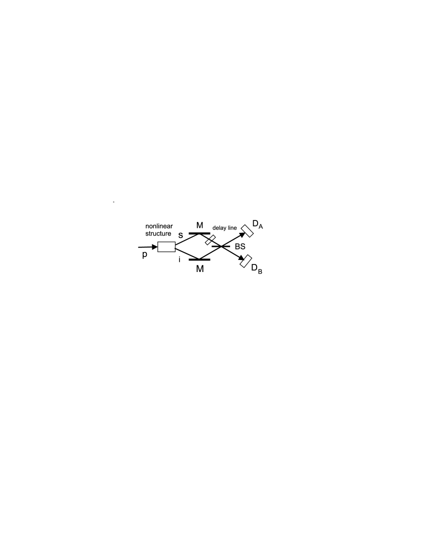
Figure 3: Scheme of Hong-Ou-Mandel interferometer. In a nonlinear structure a photon from a pump beam p is converted into a photon pair copropagating as signal (s) and idler (i) beams. After reflection from mirrors M and introduction of a mutual delay in a delay line, both photons interfere at a beam-splitter BS, and are then detected using a coincidence-count detection scheme at detectors D_A and D_B.

In order to achieve this type of interference between the signal and idler photons, we rotate polarizations of both photons such that they are the same, and subsequently introduce a relative time delay $\tau_{l}$ between the two photons. Then two photons arrive at a 50/50 % beam-splitter whose output ports are monitored by detectors. The measured coincidence-count rate $R_{c}$ is given by the number of simultaneously detected photons at detectors $D_{\rm A}$ and $D_{\rm B}$, placed at the output ports of the beam-splitter in a given time interval. There occurs quantum interference between two paths leading to a coincidence count; either a signal photon is detected by detector ${\rm D}_{A}$ and its twin idler photon by detector ${\rm D}_{B}$ or vice versa. The normalized coincidence-count rate $R_{n}$ in this interferometer can be expressed as follows:

$$R_{n}^{mn}(\tau_{l})=1-\rho^{mn}(\tau_{l}),$$ (43)

where

$$\rho^{mn}(\tau_{l}) = \frac{1}{2R_{0}^{mn}}\int_{-\infty}^{\infty}dt_{A}\,\int_{-\infty}^{\infty}dt_{B}\,$$ (44)

$${\rm Re}\left[{\cal A}^{mn}(t_{A},t_{B}-\tau_{l}){\cal A}^{mn*}(t_{B},t_{A}-\tau_{l})\right]$$

and

$$R_{0}^{mn}=\frac{1}{2}\int_{-\infty}^{\infty}dt_{A}\int_{-\infty}^{\infty}dt_{B}\left|{\cal A}^{mn}(t_{A},t_{B})\right|^{2}.$$ (45)

The symbol ${\rm Re}$ stands for real part, and the two-photon amplitude ${\cal A}^{mn}$ has been introduced in Eq. (37). Using the expressions in Eqs. (44) and (45), we arrive at:

$$\rho^{mn}(\tau_{l}) = \frac{\hbar^{2}}{8\epsilon_{0}^{2}c^{2}{\cal B}^{2}}\frac{1}{R_{0}^{mn}}{\rm Re}\Biggl{[}\int_{0}^{\infty}d\omega_{s}\,\int_{0}^{\infty}d\omega_{i}\;\omega_{s}\omega_{i}$$

$$\phi^{mn}(\omega_{s},\omega_{i})\phi^{mn*}(\omega_{i},\omega_{s})\exp(i\omega_{i}\tau_{l})\exp(-i\omega_{s}\tau_{l})\Biggr{]},$$

$$R_{0}^{mn} = \frac{\hbar^{2}}{8\epsilon_{0}^{2}c^{2}{\cal B}^{2}}\int_{0}^{\infty}d\omega_{s}\,\int_{0}^{\infty}d\omega_{i}\,\;\omega_{s}\omega_{i}|\phi^{mn}(\omega_{s},\omega_{i})|^{2}.$$

II.4 Cw-limit

If cw pumping is considered, the spectrum is described using Eq. (4). As a consequence the following expressions are obtained:

$$|\phi^{mn}(\omega_{s},\omega_{i})|^{2}=f(\omega_{s},\omega_{i})\delta^{2}(\omega_{p}-\omega_{s}-\omega_{i}).$$ (48)

In this case the second power of the Dirac delta function $\delta$ is formal, so that the above expression should be replaced by:

$$|\phi^{mn}(\omega_{s},\omega_{i})|^{2}=\lim_{T\rightarrow\infty}\frac{2T}{2\pi}f(\omega_{s},\omega_{i})\delta(\omega_{p}-\omega_{s}-\omega_{i}),$$ (49)

where the period of nonlinear interaction goes from $-T$ to $T$. Expressions for the physical quantities determined above have to be normalized by $2T$, which indicates that these quantities are related to the period of $1s$.

III Typical characteristics of the down-converted fields generated from a photonic-band-gap structure

As an example, we study the properties of a nonlinear photonic-band-gap structure composed of 25 nonlinear layers of GaN of thickness of 117 nm among which there are 24 linear layers of AlN with a thickness of 180 nm. Material characteristics of GaN and AlN can be found, e.g., in Sanford2005 ; Miragliotta1993 . This structure is resonant for the pump field at wavelength of 664.5 nm, designed to correspond to the first resonance peak near the band edge. This situation favors the efficient generation of photon pairs at roughly double the pump wavelength, at angles that correspond to the first, second, and third resonance peaks, respectively, for the down-converted fields. We assume that the GaN crystallographic $x$ axis coincides with the $z$ axis of propagation (see Fig. 1). In this configuration there is strong nonlinear interaction between TE components of the pump, signal, and idler beams. The nonlinear coefficient $d$ for this geometry is chosen to be 10 pmV$\mbox{}^{-1}$.

III.1 Cw pumping

We first consider pumping by a cw laser tuned at first resonance peak, i.e. $\lambda_{p}=664.5$ nm. A photon pair whose signal photon is emitted along the angle $\theta_{s}$ may be described by a two-photon amplitude $\ {\cal A}$ with typical shapes both in time and spectral domains. In the spectral domain, the two-photon amplitude ${\cal A}(\omega_{s},\omega_{i})$ can be written in the form $s(\omega_{s})\delta(\omega_{p}^{0}-\omega_{s}-\omega_{i})$, where the function $s(\omega_{s})$ is linearly proportional to the spectral amplitude of the signal field. This is a consequence of stationarity of the emitted down-converted fields. The probability $|{\cal A}(\tau_{s},\tau_{i})|^{2}$ of detecting a signal photon at time $\tau_{s}$ and an idler photon at time $\tau_{i}$ is shown in Fig. 4 for mode $FF$ (both photons exit the structure at $z=z_{N}$).

a)

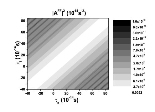
b)      

Figure 4: Probability $|{\cal A}^{FF}|^{2}$ of detecting a signal photon at time $\tau_{s}$ and its twin idler photon at time $\tau_{i}$ (a) in mode $FF$ for cw pumping is shown; cut of the graph along the line $\tau_{s}+\tau_{i}=450$ fs is shown in (b); the probability $|{\cal A}^{FF}|^{2}$ is normalized such that one photon pair is emitted, i.e. $\int d\tau_{s}\int d\tau_{i}|{\cal A}^{FF}(\tau_{s},\tau_{i})|^{2}=1$: $\theta_{s}=14$ deg; logarithmic scale on $z$ axis is used.

The shape of the probability $|{\cal A}(\tau_{s},\tau_{i})|^{2}$ can be easily understood when we consider the fact that both photons in a pair are born together at the same instant of time, and then propagate independently inside the structure. This independent zig-zag propagation increases the average time delay between the two photons, which takes into account all possible realizations of the random process of propagation of a photon that undergoes multiple bounces inside the structure. The ’random’ zig-zag propagation causes interference between different paths. This leads to a typical structure with local minima and maxima along the direction $\tau_{s}+\tau_{i}={\rm const}$; as shown in Fig. 4b. Also, the greater the difference $\tau_{s}-\tau_{i}$ the smaller the value of the two-photon amplitude ${\cal A}$ because the propagation with more zig-zags is less probable. We note that typical stripes along the direction $\tau_{s}-\tau_{i}={\rm const}$ reflect stationarity of the process.

Typical spectral properties of this structure are documented in Fig. 5, where the signal-field energy spectrum $S_{s}^{FF}$ is depicted as a function of the angle $\theta_{s}$ for field $FF$.

a)

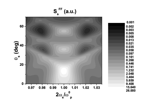
b)      

Figure 5: Energy spectrum $S_{s}^{FF}$ of mode $FF$ versus normalized signal-field frequency $2\omega_{s}/\omega_{p}^{0}$ and angle $\theta_{s}$ of emission of a signal photon is shown in (a); cuts along the lines $\theta_{s}=14$ deg (solid curve) and $\theta_{s}=28$ deg (solid curve with $*$) are shown in (b); cw pumping is assumed; logarithmic scale is used on the $z$ axis.

The spectrum $S_{s}^{FF}$ giving the probability of emission of a signal photon at frequency $\omega_{s}$ along the angle $\theta_{s}$ is a complex function in its variables because it is built up by interference of fields coming from the multilayer structure. A maximum photon-pair generation rate is obtained for $\theta_{s}\approx 13.8$ deg for degenerate frequencies ($\omega_{s}\approx\omega_{i}$). Photons from a generated photon pair can exit the structure also at $z=z_{0}$; their energy spectra $S_{s}^{FB}(\omega_{s},\theta_{s})$, $S_{s}^{BF}(\omega_{s},\theta_{s})$ and $S_{s}^{BB}(\omega_{s},\theta_{s})$ are similar to that shown in Fig. 5. This is because efficient generation of photon pairs occurs provided both the signal and idler fields are resonant in the structure so that the generated photons exit the structure at $z=z_{0}$ or $z=z_{N}$ with comparable probabilities. The signal-field intensity transmission $|T_{s}|^{2}$ as a function of normalized frequency $2\omega_{s}/\omega_{p}^{0}$ and angle $\theta_{s}$ is shown in Fig. 6 for comparison.

Figure 6: Signal-field intensity transmission $|T_{s}|^{2}$ as a function of normalized frequency $2\omega_{s}/\omega_{p}^{0}$ and angle $\theta_{s}$. Positions of peaks of resonance as they depend on the angle $\theta_{s}$ are clearly visible.

The angle-dependence of the signal-field FWHM (full-width at half maximum) $\Delta\lambda_{s}$ of the energy spectrum in wavelengths and value of energy spectrum $S_{s}^{\rm max}$ at the central frequency $\omega_{s}^{c}$ are shown in Fig. 7. High photon-pair generation rates are observed for the frequency-degenerate case ($\omega_{s}^{c}\approx\omega_{i}^{c}$) for values of the angle $\theta_{s}$ approximately equal to 14, 35, and 55 degrees. For these values of the angle $\theta_{s}$ the peaks of the signal-field intensity transmission $|T_{s}|^{2}$ cross the value $\omega_{s}$ equal to $\omega_{p}^{0}/2$ (see Fig. 6). The first and highest peaks in the signal-field energy spectra $S_{s}$ (see Fig. 7b) correspond to the case when both the signal and idler photons are tuned at the first resonance near the band edge. At this frequency, localization of the down-converted fields is maximum, and the nonlinear process is strongest. The other two sets of peaks in the signal-field energy spectra $S_{s}$ correspond to the second and third peaks in the intensity transmission $|T_{s}|^{2}$. At these frequencies, the nonlinear interaction is somewhat weaker due to smaller field intensities, i.e., slightly worse localization of the down-converted fields. The spectral FWHMs for these frequency-degenerate emissions lye in the interval from 10 nm to 15 nm (see Fig. 7a). For these values of the angle $\theta_{s}$ the best available constructive interference in the structure occurs. In a relatively narrow frequency interval the signal and idler fields are enhanced by constructive interference. Outside this frequency interval, destructive interference occurs. For the other values of the angle $\theta_{s}$ constructive interference is less pronounced, the range of frequencies having constructive interference is broader, and spectral shapes with several peaks may occur (see Fig. 5b). We thus obtain down-converted fields with spectral FWHMs reaching even 80nm (see Fig. 7a). In this case the FWHM indicates the entire active width, which might include several peaks. However, photon-pair generation rates are low in this case.

a)      

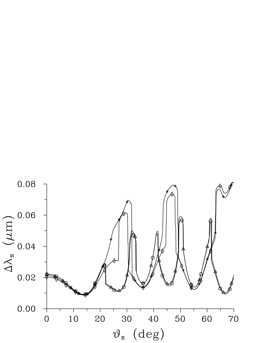
b)      

Figure 7: FWHM $\Delta\lambda_{s}$ (a) and maximum value $S_{s}^{\rm max}$ at the central frequency $\omega_{s}^{c}$ (b) for the signal-field energy spectrum $S_{s}(\omega_{s})$ of modes $FF$ ($*$), $FB$ ($\triangle$), $BF$ ($\circ$), and $BB$ ($\diamond$) as functions of the angle $\theta_{s}$ of emission of a signal photon are shown; cw pumping is assumed.

Quantum correlations (entanglement) between the signal and idler photons in a photon pair are visible in the profile of the normalized coincidence-count rate $R_{n}(\tau_{l})$ in a Hong-Ou-Mandel interferometer (see Fig. 8 for mode $FF$).

a)

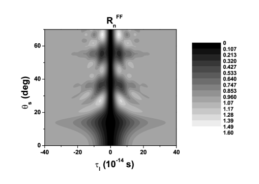
b)      

Figure 8: (a) Normalized coincidence-count rate $R_{n}^{FF}$ of mode $FF$ in Hong-Ou-Mandel interferometer as a function of relative time delay $\tau_{l}$ and angle $\theta_{s}$ of emission of a signal photon; (b) cuts along the lines $\theta_{s}=14$ deg (solid curve) and $\theta_{s}=28$ deg (solid curve with *); cw pumping is assumed.

For values of the angle $\theta_{s}$ with strong constructive interference ($\theta_{s}\approx 14,35,55$ deg) this profile is given by a relatively broad dip (see Fig. 8b). On the other hand, oscillating curves with several local minima and maxima characterize profiles of the normalized coincidence-count rates $R_{n}(\tau_{l})$ for other values of the angle $\theta_{s}$. A typical profile for this case is shown in Fig. 8b. These profiles reflect broader spectra of the down-converted fields along these angles as well as a nonzero difference of the central frequencies $\omega_{s}^{c}$ and $\omega_{i}^{c}$ of the signal and idler fields. Period of these oscillations is proportional to $1/(\omega_{s}^{c}-\omega_{i}^{c})$.

Position $\tau_{l}^{c}$ of the central dip, its FWHM $\Delta\tau_{l}$, and visibility $V$ of the normalized coincidence-count rate $R_{n}$ as functions of the angle $\theta_{s}$ are shown in Fig. 9.

a)      

b)      

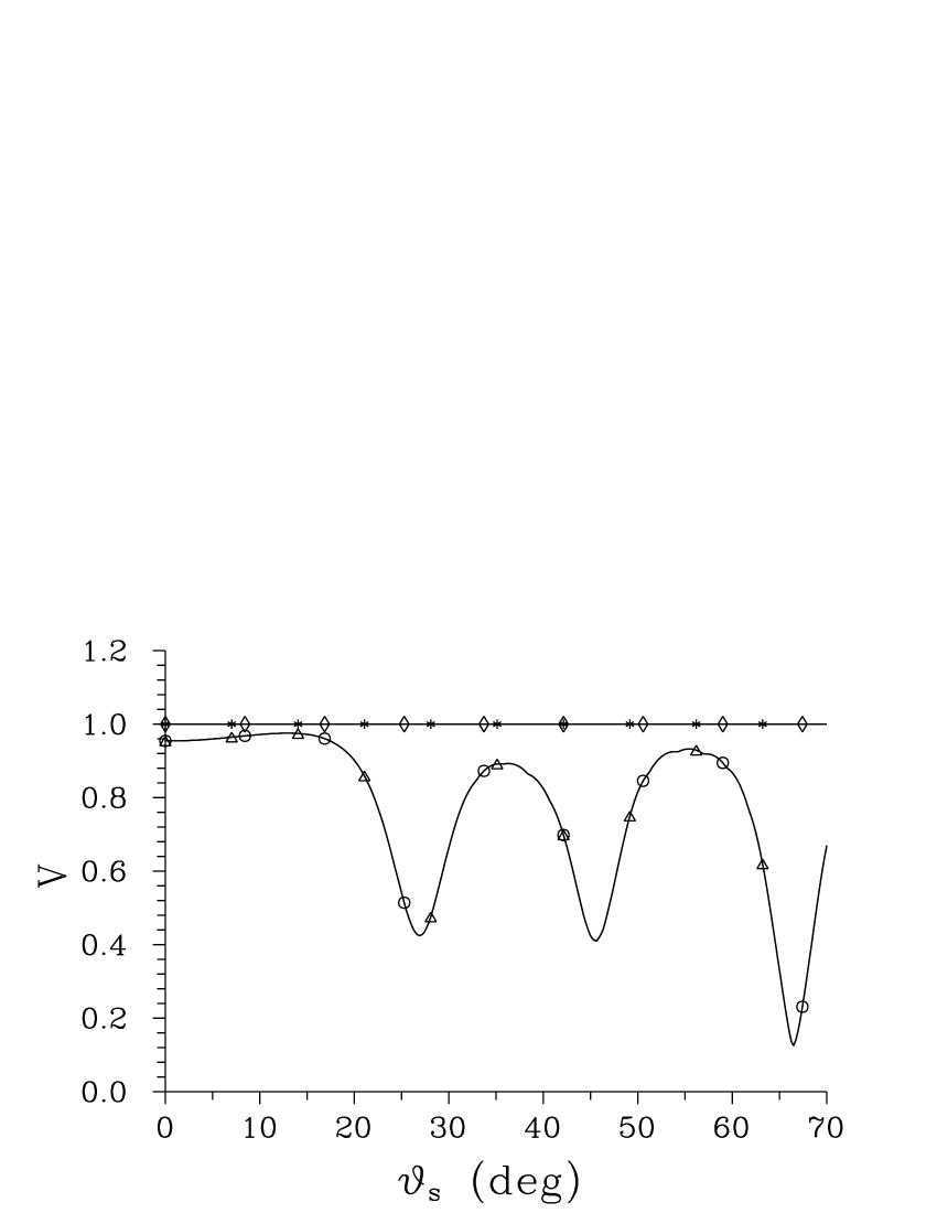
c)      

Figure 9: Position $\tau_{l}^{c}$ of the central dip (a), its visibility $V$ [$V=\frac{\rho}{(2-\rho)}$] (b), and FWHM $\Delta\tau_{l}$ of the dip (c) for the normalized coincidence-count rate $R_{n}(\tau_{l})$ in Hong-Ou-Mandel interferometer in modes $FF$ ($*$), $FB$ ($\triangle$), $BF$ ($\circ$), and $BB$ ($\diamond$) as functions of the angle $\theta_{s}$ of emission of a signal photon; cw pumping is assumed.

We can see in Fig. 9a that the maximum overlap of the signal and idler photon fields is reached for a nonzero mutual time delay $\tau_{l}$ for nonsymmetric modes $FB$ and $BF$. This means that the signal and idler photons exit the structure with a small mutual time delay. This nonzero mutual time delay means that interference effects inside the structure prefer the generation of photon pairs from nonlinear layers positioned closer to one edge of the structure, or in any case approximately co-located. The visibility $V$ of the coincidence-count rate $R_{n}$ equal to one is naturally observed for symmetric modes $FF$ and $BB$. Values of the visibility $V$ better than 0.9 can also be reached in nonsymmetric modes $FB$ and $BF$ provided that the fields are generated along the angles $\theta_{s}$ in the vicinity of those with a strong constructive interference. The structure of quantum correlations between the signal and idler fields in time domain is complex and prevents the visibility $V$ from reaching higher values along the angles $\theta_{s}$, where there are broad spectra of the down-converted fields. The width $\Delta\tau_{l}$ of the dip in the normalized coincidence-count rate $R_{n}(\tau_{l})$ determines the entanglement time, i.e. the time interval in which both photons can be detected. The FWHM $\Delta\tau_{l}$ of the central dip for the structure ranges from 50 fs for values of the angle $\theta_{s}$ with broad spectra of the down-converted fields, to 150-250 fs for values of the angle $\theta_{s}$ at where strong constructive interference occurs (see Fig. 9c).

III.2 Pumping by an ultrashort pulse

We now assume that the structure is pumped by an ultrashort pulse with an unchirped Gaussian profile [see Eq.(2)] having pulse duration $\tau_{p}$ equal to 200 fs, and central (carrier) frequency $\omega_{p}^{0}$ at the wavelength of 664.5 nm. The squared modulus $|E_{p}|^{2}$ of the incident pump-field amplitude spectrum ${\bf E}_{p_{F},TE}(\omega_{p})$ fits well into the peak of resonance of the pump-field intensity transmission $|T_{p}(\omega_{p})|^{2}$, as depicted in Fig. 10.

Figure 10: Pump-field intensity transmission $|T_{p}|^{2}$ (solid curve) and squared modulus $|{\bf E}_{p_{F},TE}|^{2}$ of the pump-field amplitude spectrum (solid curve with $*$) as functions of the normalized pump-field frequency $\omega_{p}/\omega_{p}^{0}$.

Only signal and idler photons with frequencies $\omega_{s}$ and $\omega_{i}$ for which the sum $\omega_{s}+\omega_{i}$ lyes within the pump-pulse spectrum may be generated. The allowed values of the frequencies $\omega_{s}$ and $\omega_{i}$ are indicated in the graph of the probability $|\phi(\omega_{s},\omega_{i})|^{2}$ of emitting a signal photon at frequency $\omega_{s}$ and its twin at frequency $\omega_{i}$. A typical shape of the probability $|\phi(\omega_{s},\omega_{i})|^{2}$ is shown in Fig. 11 for mode $FF$.

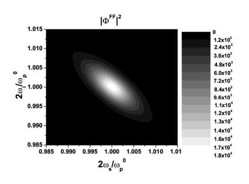
Figure 11: The probability $|\phi^{FF}|^{2}$ of having a photon pair in mode $FF$ with a signal photon at the normalized frequency $2\omega_{s}/\omega_{p}^{0}$ and an idler photon at the normalized frequency $2\omega_{i}/\omega_{p}^{0}$ for pulsed pumping; the probability $|\phi^{FF}|^{2}$ is normalized such that one photon pair is emitted, i.e. $4\int d\omega_{s}\int d\omega_{i}|\phi^{FF}(\omega_{s},\omega_{i})|^{2}(\omega_{p}^{0})^{2}=1$; $\theta_{s}=14$ deg.

We note that the shape of the probability $|\phi(\omega_{s},\omega_{i})|^{2}$ in Fig. 11 may be considered as being composed of many curves defined above the lines $\omega_{s}+\omega_{i}=\omega_{p}={\rm const}$, and it may be assumed to be linearly proportional to those characterizing cw pumping at the frequency $\omega_{p}$. The probability $|{\cal A}(\tau_{s},\tau_{i})|^{2}$ of detecting a signal photon at time $\tau_{s}$ and its twin at time $\tau_{i}$ depicted in Fig. 12 shows that both signal and idler photons occur in sharp time windows as a consequence of pumping by an ultrashort pulse.

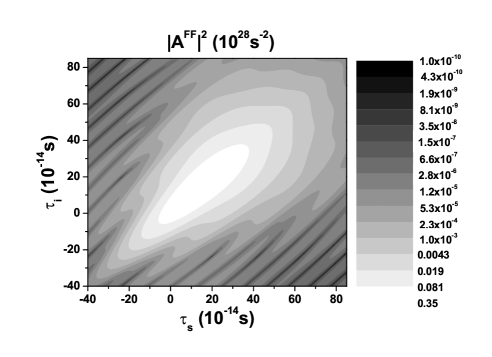
Figure 12: The probability $|{\cal A}^{FF}|^{2}$ of detecting a signal photon at time $\tau_{s}$ and its twin idler photon at time $\tau_{i}$ in mode $FF$ for pulsed pumping; the probability $|{\cal A}^{FF}|^{2}$ is normalized such that one photon pair is emitted, i.e. $\int d\tau_{s}\int d\tau_{i}|{\cal A}^{FF}(\tau_{s},\tau_{i})|^{2}=1$; $\theta_{s}=14$ deg; logarithmic scale is used on the $z$ axis.

The probability $|{\cal A}(\tau_{s},\tau_{i})|^{2}$ has a typical droplet shape that reflects the fact that the longer the photons from a pair propagate inside the structure, the greater the average difference of the occurrence times $\tau_{s}$ and $\tau_{i}$ of the photons. The structure with local minima and maxima farther from the diagonal in Fig. 12 reflects interference in the layered structure.

Because the pump-pulse amplitude spectrum ${\bf E}_{p_{F},TE}$ fits well into the peak of resonance of the structure, and the emitted frequencies of the down-converted fields have also to fit into the structure, the energy spectra of the signal and idler fields with pulsed pumping are very similar to those obtained for cw pumping. Also, the behavior of photon pairs generated by pulsed pumping in the Hong-Ou-Mandel interferometer is similar to that observed with cw pumping; only the visibilities $V$ of the normalized coincidence-count rates $R_{n}(\tau_{l})$ are slightly worse.

The signal and idler fields are now emitted in the form of ultrashort, pulsed fields in multimode Fock states. A typical dependence of the signal-field photon flux $N_{s}^{FF}$ at time $\tau_{s}$ and angle $\theta_{s}$ is shown in Fig. 13. Fig. 13 suggests that the photon flux $N_{s}$ typically spreads to longer times as a consequence of zig-zag movement, i.e. multiple scattering, of photons inside the structure.

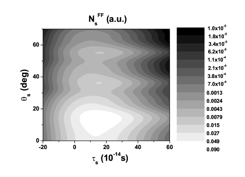
Figure 13: Photon flux ${\cal N}_{s}^{FF}$ of mode $FF$ as a function of time $\tau_{s}$ of detection of a signal photon and angle $\theta_{s}$ of emission of a signal photon; pulsed pumping is assumed; logarithmic scale is used on the $z$ axis.

Time delay $\tau_{s}^{c}$ and FWHM $\Delta\tau_{s}$ of the pulsed signal field as well as photon flux $N_{s}^{\rm max}$ at the center of the pulsed field as they depend on the angle $\theta_{s}$ are depicted in Fig. 14.

a)      

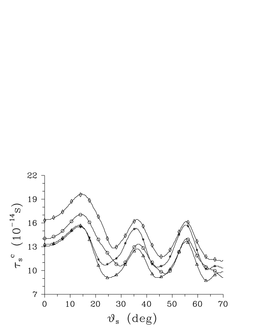
b)      

c)      

Figure 14: Time delay $\tau_{s}^{c}$ (a), FWHM $\Delta\tau_{s}$ (b), and photon flux $N_{s}^{\rm max}$ at the center ($\tau_{s}=\tau_{s}^{c}$) for the pulsed signal field in modes $FF$ ($*$), $FB$ ($\triangle$), $BF$ ($\circ$), and $BB$ ($\diamond$) as they depend on the angle $\theta_{s}$ of emission of a signal photon; pulsed pumping is assumed.

The time delay $\tau_{s}^{c}$ of the signal pulse with respect to the pump pulse ranges from 70 fs to 200 fs. It reaches its maximum values for values of the angle $\theta_{s}$ with strong constructive interference ($\theta_{s}\approx 14,35,55$ deg). FWHM $\Delta\tau_{s}$ of the signal pulse goes from 270 fs to 320 fs. The narrower the spectrum of the signal field (given by $\Delta\lambda_{s}$ in wavelengths) the greater the signal-field pulse duration $\Delta\tau_{s}$ (compare Figs. 7a and 14b). The largest value of the photon flux $N_{s}^{\max}$ can be reached for the angle $\theta_{s}$ equal to 13.8 deg (see Fig. 14c).

These results clearly show that the considered photonic-band-gap structure maintains a pulsed character of the nonlinear process and allows generation of pulsed down-converted fields with an ultrashort duration. Such pulsed fields are required in many experiments with photon pairs in which time synchronization of several photon pairs is necessary.

III.3 Efficiency of the nonlinear process

The model that we have developed is one dimensional with respect to the spatial coordinates, and does not include all aspects (especially those related to transverse profiles of the interacting optical fields) of the nonlinear process in a real structure. For this reason we do not determine the absolute values of photon-pair generation rates. Instead, we judge the efficiency of the suggested structure (stemming from constructive interference of the interacting optical fields) with respect to an ideal reference structure which fully exploits the nonlinearity, but does not rely on interference.

This reference structure has formally all linear indices of refraction equal to one, so effects on the boundaries between layers are suppressed. It is also assumed that the nonlinear process is fully phase matched. The orientations of nonlinear layers, as well as polarizations of the interacting optical fields, are such that the greatest nonlinear effect occurs. A photon pair emitted from this structure is described by the following output state $|\psi\rangle_{s,i}^{\rm ref}$ [compare Eq. (20)]:

$$|\psi\rangle_{s,i}^{\rm ref} = -\frac{i}{2\sqrt{2\pi}c}\int_{0}^{\infty}\,d\omega_{p}\int_{0}^{\infty}\,d\omega_{s}\sqrt{\omega_{s}}\sqrt{\omega_{p}-\omega_{i}}$$

$$\mbox{}|{\bf E}_{p_{F}}^{(+)}(0,\omega_{p})|\sum_{l=1}^{N}\max({\bf d}^{(l)})L_{l}\hat{a}_{s}^{\dagger}(\omega_{s})\hat{a}_{i}^{\dagger}(\omega_{p}-\omega_{s})|{\rm vac}\rangle,$$

where $\hat{a}_{s}^{\dagger}(\omega_{s})$ [$\hat{a}_{i}^{\dagger}(\omega_{i})$] denotes a creation operator of a photon in the signal [idler] field. The function $\max$ used in Eq. (LABEL:50) gives the maximum value from the elements of a tensor in its argument.

The relative photon-pair generation rate $\eta^{mn}(\omega_{s})$ of a pair with a signal photon at frequency $\omega_{s}$ in mode $mn$ is then given as:

$$\eta^{mn}(\omega_{s})=\frac{S_{s}^{mn}(\omega_{s})}{S_{s}^{\rm ref}(\omega_{s})},$$ (51)

where the signal-field energy spectrum $S_{s}^{mn}$ is given in Eq. (35), and the signal-field energy spectrum $S_{s}^{\rm ref}$ of the reference structure is determined in the same way using the output state $|\psi\rangle_{s,i}^{\rm ref}$ written in Eq. (LABEL:50).

The relative photon-pair generation rates $\eta^{FF}$, $\eta^{FB}$, $\eta^{BF}$, and $\eta^{BB}$ for the signal-field frequency $\omega_{s}=\omega_{p}^{0}/2$ as a function of the angle $\theta_{s}$ are shown in Fig. 15 assuming cw pumping.

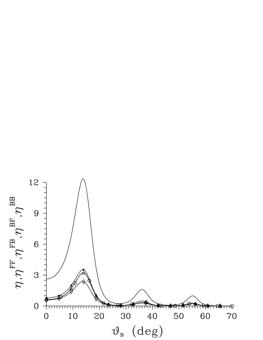
Figure 15: Relative photon-pair generation rates $\eta^{FF}$ ($*$), $\eta^{FB}$ ($\triangle$), $\eta^{BF}$ ($\circ$), $\eta^{BB}$ ($\diamond$), and overall relative photon-pair generation rate $\eta$ ($\eta=\eta^{FF}+\eta^{FB}+\eta^{BF}+\eta^{BB}$) at the signal-field frequency $\omega_{s}=\omega_{p}^{0}/2$ for cw pumping as a function of angle $\theta_{s}$ of emission of a signal photon.

The relative photon-pair generation rates for pulsed pumping are lower in comparison with cw pumping, because frequencies at the edges of the pump-field spectrum have lower efficiencies than those in the middle. Despite this, the considered pulsed pumping has the overall relative photon-pair generation rate $\eta$ equal to 9, whereas $\eta=12.5$ for cw pumping for $\theta_{s}\approx 13.8$ deg. The structure that we consider is approximately 12 times more efficient than the reference structure, provided we consider all the emitted photon pairs (given by the overall relative photon-pair generation rate $\eta$ in Fig. 15). Even when we restrict ourselves only to the mode $FF$, we still have an enhancement of the nonlinear process by a factor of three. For comparison purposes, one layer of GaN of thickness $25\times 117$ nm (i.e., containing the same amount of nonlinear material as our structure) has the overall relative photon-pair generation rate $\eta$ equal to 0.09 for values of the angle $\theta_{s}$ less than 20 deg. The inclusion of linear layers of AlN inside the structure and the accompanying interference effects thus increase the photon-pair generation rates by two orders of magnitude.

IV Conclusion

We have developed a quantum model of spontaneous parametric down-conversion (generating entangled photon pairs) in one-dimensional, nonlinear, layered media. Using the model we have determined a two-photon amplitude, and we have provided measurable characteristics of the down-converted fields: marginal signal and idler energy spectra, time-dependent photon fluxes of the signal and idler fields, coincidence-count interference patterns in the Hong-Ou-Mandel interferometer, and photon-pair generation rates.

A specific structure was suggested as an efficient source of photon pairs, and interference effects of the interacting fields can enhance the photon-pair generation rates by as much as two hundred times. The widths of the spectra of the down-converted fields and entanglement time of photons in a pair depend strongly on the angle of emission, and vary from 10 nm to 80 nm and from 50 fs to 250 fs, respectively. Pumping the structure with an ultrashort pulse of time duration of several hundreds of fs can lead to the generation of pulsed signal and idler fields extending over several hundreds of fs.

Therefore, we conclude that nonlinear one-dimensional photonic-band-gap structures represent a promising, new efficient source of photon pairs.

- (1) C.K. Hong, Z.Y. Ou, and L. Mandel, Phys. Rev. Lett. 59, 2044 (1987).
- (2) L. Mandel, E. Wolf, Optical Coherence and Quantum Optics (Cambridge Univ. Press. Cambridge, 1995).
- (3) J. Peřina, Z. Hradil, and B. Jurčo, Quantum Optics and Fundamentals of Physics (Kluwer, Dordrecht, 1994).
- (4) D. Bouwmeester, J.-W. Pan, K. Mattle, M. Eibl, H. Weinfurter, and A. Zeilinger, Nature 390, 575 (1997).
- (5) D. Bouwmeester, J.-W. Pan, M. Daniell, H. Weinfurter, and A. Zeilinger, Phys. Rev. Lett. 82, 1345 (1999).
- (6) D. Bouwmeester, A. Ekert, and A. Zeilinger (Eds. The Physics of Quantum Information (Springer, Berlin, 2000).
- (7) D. Bruß, N. Lütkenhaus, in Applicable Algebra in Engineering, Communication and Computing Vol. 10 (Springer, Berlin, 2000); p. 383.
- (8) A. Migdall, Physics Today 1, 41 (1999).
- (9) P.G. Kwiat, E. Waks, A.G. White, I. Appelbaum, and P.H. Eberhard, Phys. Rev. A 60, R773 (1999).
- (10) P.G. Kwiat, Nature 412, 866 (2001).
- (11) Y. Nambu, K. Usami, Y. Tsuda, K. Matsumoto, K. Nakamura, Phys. Rev. A 66, 033816 (2002).
- (12) J.H. Shapiro and N.C. Wong, J. Opt. B: Quantum Semiclass. Opt. 2, L1 (2000).
- (13) C.E. Kuklewicz, M. Fiorentino, G. Messin, F.N.C. Wong, and J. Shapiro, Opt. Express 13, 127 (2005).
- (14) P. Trojek, C. Schmid, M. Bourennane, H. Weinfurter, and C. Kurtsiefer, Opt. Express 12, 276 (2004).
- (15) M. Bertolotti, C.M. Bowden, and C. Sibilia, Nanoscale Linear and Nonlinear Optics, AIP Vol. 560 (AIP, Melville, 2001).
- (16) E. Yablonovitch, Phys. Rev. Lett. 58, 2059 (1987).
- (17) S. John, Phys. Rev. Lett. 58, 2486 (1987).
- (18) J.D. Joannopoulos, R.D. Meade, and J.N. Winn, Photonic Crystals (Princeton University Press, Princeton, 1995).
- (19) K. Sakoda, Optical Properties of Photonic Crystals (Springer, NewYork, 2005), 2nd ed.
- (20) A.N. Vamivakas, B.E.A. Saleh, A.V. Sergienko, and M.C. Teich, Phys. Rev. A 70, 043810 (2004).
- (21) M. Centini, J. Peřina Jr., L. Sciscione, C. Sibilia, M. Scalora, M.J. Bloemer, and M. Bertolotti, Phys. Rev. A 72, 033806 (2005).
- (22) X. Li, P.L. Voss, J.E. Sharping, and P. Kumar, Phys. Rev. Lett. 94, 053601 (2005).
- (23) J. Fulconis, O. Alibart, W.J. Wadsworth, P. S. Russell, and J. G. Rarity, Opt. Express 13, 7572 (2005).
- (24) T.E. Keller and M.H. Rubin, Phys. Rev. A 56, 1534 (1997).
- (25) J. Peřina Jr, A.V. Sergienko, B.M. Jost, B.E.A. Saleh, and M.C. Teich, Phys. Rev. A 59, 2359 (1999).
- (26) G. Di Giuseppe, L. Haiberger, F. De Martini and A.V. Sergienko, Phys. Rev. A 56, R21 (1997).
- (27) W.P. Grice, R. Erdmann, I.A. Walmsley, and D. Branning, Phys. Rev. A 57, R2289 (1998).
- (28) P. Yeh, Optical Waves in Layered Media (Wiley, New York, 1988).
- (29) W. Vogel, D.G.Welsch, S. Walentowicz, Quantum Optics (Wiley-VCH, Weinheim, 2001).
- (30) G. D’Aguanno, N. Mattiucci, M. Scalora, M.J. Bloemer, and A.M. Zheltikov, Phys. Rev. E 70, 016612 (2004).
- (31) N.A. Sanford, A.V. Davidov, D.V. Tsvetkov, A.V. Dmitriev, S. Keller, U.K. Mishra, S.P. DenBaars, S.S. Park, J.Y. Han and R.J. Molnar, J. Apl. Phys. 97, 053512 (2005).
- (32) J. Miragliotta, D.K. Winckenden, T.J. Kistenmacher, W. A. Bryden, J. Opt. Soc. Am. B 10, 1447 (1993).