Comb entanglement in quantum spin chains

Abstract

Bipartite entanglement in the ground state of a chain of $N$ quantum spins can be quantified either by computing pairwise concurrence or by dividing the chain into two complementary subsystems. In the latter case the smaller subsystem is usually a single spin or a block of adjacent spins and the entanglement differentiates between critical and non-critical regimes. Here we extend this approach by considering a more general setting: our smaller subsystem $S_{A}$ consists of a comb of $L$ spins, spaced $p$ sites apart. Our results are thus not restricted to a simple ‘area law’, but contain non-local information, parameterized by the spacing $p$. For the XX model we calculate the von-Neumann entropy analytically when $N\rightarrow\infty$ and investigate its dependence on $L$ and $p$. We find that an external magnetic field induces an unexpected length scale for entanglement in this case.

I Introduction

Quantum phase transitions at zero temperature correspond to a fundamental restructuring of a system’s ground state. In quantum spin chains these transitions occur as an external parameter (e.g. a magnetic field) is varied book , and are manifested as a marked change in the decay of quantum correlations: algebraic at the critical point and exponential away from it. The amount of entanglement present in the ground state is expected to depend significantly on whether the system is critical or not, since at a critical point all the constituent parts of the system must be non-locally correlated and thus entangled pra66tjo2002 ; n416ao2002 ; prl90gv2003 ; qic4jil2004 ; pra71vp2005 ; pra71mfy2005 .

Unfortunately, it is not yet clear how to measure entanglement in general pra70rs2004 . At present, we only understand fully how to quantify bipartite entanglement pra53chb1996 . It is natural, therefore, to try to extract as much information as possible about entanglement in this context. Ways of doing this have recently been the focus of considerable attention. One possibility is the following. From a chain of $N$ spin-$\frac{1}{2}$ particles select two, compute their reduced density matrix, and then obtain the associated concurrence prl80wt1998 . This is a function of the separation between the selected spins. Despite the fact that the concurrence is only a short-range measure (it vanishes if the spins are farther apart than next-nearest neighbors), this approach has been applied to detect phase transitions in a variety of situations pra66tjo2002 ; n416ao2002 ; pra71vp2005 . A second possibility is to measure the entanglement between a single spin and the rest of the chain. This has also been related to the presence of a critical point pra66tjo2002 .

The problem with these methods, which involve a small number of spins, is that they do not take into account the fact that entanglement is shared between many parties, i.e. they provide little information regarding the non-local nature of entanglement. This deficiency is shared by another much-studied bipartite division of the spin chain, namely that between a block of $L$ adjacent spins and the remaining $N-L$ prl90gv2003 ; qic4jil2004 . In the limit $N\rightarrow\infty$, the entanglement entropy has in this case been computed analytically using the theory of Toeplitz determinants (for the XX model) jsp116bqj2004 ; fisher , conformal field theory prl92vek2004 , and from averages over ensembles of random matrices cmp252jpk2004 . For one-dimensional chains it has been shown that as $L\rightarrow\infty$ the entropy tends to a constant value away from critical points, and that it diverges like $\ln L$ at phase transitions. For critical $d$-dimensional spin-lattices this ‘block’ entanglement has been proven to grow like $L^{d-1}\ln L$ under certain conditions prl96mmw2006 , while for a gapped system one expects an area scaling law due to the finite correlation length cramer . Such a direct relation between entanglement and area is known to hold in harmonic lattices pra73mc2006 . All these results indicate that, at least for large blocks, the entanglement comes mostly from the boundary.

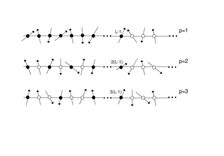
Figure 1: The comb division illustrated for three different values of the spacing $p$. In all cases one subsystem ($S_{A}$, denoted by black circles) contains $L$ spins and the other ($S_{B}$, denoted by empty circles) contains the rest of the chain. We have written explicitly the label of the last of the $L$ spins (the label of the first spin is $0$). The first case, $p=1$, corresponds to the well known ‘block’ division.

Our purpose here is to introduce a new geometry in which to study bipartite entanglement in quantum spin chains. We divide the chain into two subsystems, $S_{A}$ and $S_{B}$, as follows. $S_{A}$ consists of $L$ equally spaced spins, such that the spacing between the spins in this subsystem corresponds to $p$ sites on the chain. $S_{B}$ then contains the remaining $N-L$ spins. (Obviously this only makes sense if $N>(L-1)p$.) $S_{A}$ can be visualized as a comb with $L$ teeth. This geometry enables us to study non-local entanglement effects by varying the spacing $p$.

Three possible divisions are illustrated in Fig.1. For $p=1$ we recover the simple ‘block’ arrangement, which, as was noted above, has already been the subject of extensive investigation. In this case the subsystems $S_{A}$ and $S_{B}$ are only ‘in contact’ near their common border, and as a result, for large values of $L$, the dependence of the entanglement on $L$ is minimal. For $p>1$ the entanglement between $S_{A}$ and $S_{B}$ is shared between many different sites and it then grows linearly with $L$, to leading order as $L\rightarrow\infty$. The $\log L$ term that dominates when $p=1$ appears as a secondary correction when $p>1$. As an example, we investigate how the comb entanglement in the XX model depends on the spacing $p$ when $L$ is fixed and show that this reveals the emergence of a new length-scale determined by the external magnetic field.

II Block entropy

The XY spin chain in an external uniform magnetic field $h$ has as its Hamiltonian

$$H=\sum_{j=0}^{N-1}\left(\frac{1+\gamma}{2}\,\sigma_{j}^{x}\sigma_{j+1}^{x}+\frac{1-\gamma}{2}\,\sigma_{j}^{y}\sigma_{j+1}^{y}\right)-h\sum_{j=0}^{N}\sigma_{j}^{z},$$ (1)

where $(\sigma_{j}^{x},\sigma_{j}^{y},\sigma_{j}^{z})$ are the usual Pauli matrices. When $\gamma=0$ this system is called the XX model and when $\gamma=1$ it is the Ising model. It is an integrable model pra2eb1970 which displays both critical and non-critical regimes. In the $\gamma-h$ phase diagram the lines $h=\pm 1$ and the segment $\gamma=0,\lvert h\rvert<1$ are critical, while all other regions are non-critical. For simplicity, we will restrict our analysis mainly to the XX model and will come back to the general case towards the end.

Since the XX ground state is just a (non-entangled) ferromagnet for $\lvert h\rvert>1$, we will only consider its critical regime. A more convenient parameter in that case is the angle $k$ defined by

$$h=\cos k,\quad k\in[0,\pi].$$ (2)

We denote by $|\Psi\rangle$ the ground state of this system and introduce the Jordan-Wigner (JW) transform at each site of the lattice,

$$m_{2l+1}=\left(\prod_{j=0}^{l-1}\sigma_{j}^{z}\right)\sigma_{l}^{x},\quad m_{2l}=\left(\prod_{j=0}^{l-1}\sigma_{j}^{z}\right)\sigma_{l}^{y}.$$ (3)

Given any product of an odd number of JW operators, we can see from the symmetry of the Hamiltonian that its expectation value with respect to $|\Psi\rangle$ vanishes. Wick’s theorem and the relation $\langle\Psi|m_{j}m_{k}|\Psi\rangle=\delta_{jk}+i(C_{N})_{jk}$, where $C_{N}$ is called the correlation matrix, allow for the calculation of the expectation value of a product of any number of JW operators.

The matrix $C_{N}$ factorizes into a direct product,

$$C_{N}=T[g]\otimes\left(\begin{array}[]{cc}0&1\\ -1&0\\ \end{array}\right),$$ (4)

where $T[g]$ is the matrix

$$(T[g])_{jk}=\tilde{g}_{j-k},\quad\tilde{g}_{n}=\frac{1}{2\pi}\int_{0}^{2\pi}g(\theta)e^{-in\theta}d\theta.$$ (5)

The function $g(\theta)$ is called the symbol of the Toeplitz matrix $T[g]$. For the XX chain it is given by

$$g(\theta)=\begin{cases}1&\text{if }-k\leq\theta<k,\\ -1&\text{otherwise}.\end{cases}$$ (6)

Following the calculation presented in jsp116bqj2004 , the entropy of subsystem $S_{A}$ is obtained as a contour integral in the complex plane:

$$E=\lim_{\epsilon\rightarrow 0^{+}}\lim_{\delta\rightarrow 0^{+}}\frac{1}{2\pi i}\oint_{c(\epsilon,\delta)}e(1+\epsilon,\lambda)\frac{d\ln D_{A}(\lambda)}{d\lambda}d\lambda,$$ (7)

where $D_{A}(\lambda)={\rm det}(\lambda I-T_{A}[g])$ involves the matrix $T_{A}[g]$, which is obtained from the original matrix $T[g]$ by removing the rows and columns that correspond to sites in $S_{B}$, and

$$e(x,y)=-\frac{x+y}{2}\log_{2}\left(\frac{x+y}{2}\right)-\frac{x-y}{2}\log_{2}\left(\frac{x-y}{2}\right).$$ (8)

The contour of integration $c(\epsilon,\delta)$ approaches the interval $[-1,1]$ as $\epsilon$ and $\delta$ tend to zero without enclosing the branch points of $e(1+\epsilon,\lambda)$.

When $S_{A}$ corresponds to $L$ consecutive spins, i.e. in the block case, $T_{A}$ is simply a block inside $T$ and thus is also a Toeplitz matrix. This allowed Jin and Korepin jsp116bqj2004 to obtain the corresponding entropy by using a proved instance of the Fisher-Hartwig conjecture relating to the asymptotics of Toeplitz determinants fisher . This states that in the limit of large blocks we have

$$\ln D_{A}(\lambda)=c_{0}L+\beta^{2}\ln L+O(1),$$ (9)

where

$$c_{0}(\lambda)=\frac{1}{2\pi}\int_{0}^{2\pi}\ln\bigl{(}\lambda-g(\theta)\bigr{)}d\theta.$$ (10)

The coefficient $\beta(\lambda)$ may be calculated by writing the symbol as

$$\lambda-g(\theta)=\phi(\lambda)t_{\beta}(\theta-k)t_{-\beta}(\theta+k),$$ (11)

with $t_{\beta}(\theta)=e^{-i\beta(\pi-\theta)}$ and

$$\phi(\lambda)=(\lambda+1)\left(\frac{\lambda+1}{\lambda-1}\right)^{-k/\pi},$$ (12)

and hence it is given by

$$\beta(\lambda)=-\frac{1}{2\pi i}\ln\left(\frac{\lambda+1}{\lambda-1}\right).$$ (13)

As a consequence of the Fisher-Hartwig conjecture the entanglement as $L\rightarrow\infty$ is

$$E(L)=\mathcal{E}_{1}L+\mathcal{E}_{2}\ln L+O(1).$$ (14)

Because of the simplicity of the function $g(\theta)$ all the relevant quantities can be evaluated. In particular, we have

$$c_{0}(\lambda)=\frac{1}{\pi}\bigl{[}k\ln(\lambda-1)+(\pi-k)\ln(\lambda+1)\bigr{]},$$ (15)

and by substituting this into (7) we see that the leading order term $\mathcal{E}_{1}$ actually vanishes because

$$e(1,1)=e(1,-1)=0.$$ (16)

Therefore the dependence upon $L$ is only logarithmic, with a prefactor $\mathcal{E}_{2}$ which is obtained from (7). It turns out that when $p>1$ the leading order contribution does not vanish. The next section is devoted to its computation.

III Comb entropy

The choice we propose for the subsystem $S_{A}$ also leads to a Toeplitz structure for the matrix $T_{A}$. We single out those spins whose label is a multiple of an integer $p$, and thus we have

$$(T_{A})_{jk}=\tilde{g}_{pj-pk}=\frac{1}{2\pi}\int_{0}^{2\pi}g(\theta)e^{-ip(j-k)\theta}d\theta.$$ (17)

This is not yet in the Toeplitz form. We must first find a function $g_{p}(\theta)$ such that

$$\int_{0}^{2\pi}g(\alpha)e^{-ipn\alpha}d\alpha=\int_{0}^{2\pi}g_{p}(\alpha)e^{-in\alpha}d\alpha,$$ (18)

and this will be the symbol of $T_{A}$. Multiplying (18) by $e^{in\theta}$ with $0\leq\theta<2\pi$, summing over $n$ and using the Poisson summation formula we arrive at

$$g_{p}(\theta)=\frac{1}{p}\sum_{n=0}^{p-1}g\left(\frac{\theta}{p}+\frac{2n\pi}{p}\right),$$ (19)

so the value of $g_{p}$ at the point $\theta$ is obtained as the average value of $g$ over the $p$ vertices of a regular polygon.

This average is not hard to calculate. It is easy to see that for each $k$ the function $g_{p}(\theta)$ is piecewise constant and even, with jumps at the critical points $\pm\theta^{\ast}$ given by

$$[0,\pi)\ni\theta^{\ast}=\min\{\alpha,2\pi-\alpha\},\quad\alpha=pk\;\bmod 2\pi.$$ (20)

Its values are

$$g_{p}(\theta)=\frac{2}{p}-1+\frac{4}{p}\left\llbracket\frac{pk}{2\pi}\right\rrbracket+\begin{cases}0&\text{if }-\theta^{\ast}\leq\theta<\theta^{\ast}\\ 2s/p&\text{otherwise },\end{cases}$$ (21)

where the brackets $\llbracket\cdot\rrbracket$ denote the integer part and

$$s={\rm sign}\{\alpha-\pi\}.$$ (22)

The entanglement will now depend on the spacing:

$$E(L;p)=\mathcal{E}_{1}(p)L+\mathcal{E}_{2}(p)\ln L+O(1)$$ (23)

as $L\rightarrow\infty$. To calculate it to leading order we only need the integral

$$c_{0}=\frac{1}{2\pi}\int_{0}^{2\pi}\ln\bigl{(}\lambda-g_{p}(\theta)\bigr{)}d\theta,$$ (24)

and this leads to

$$\mathcal{E}_{1}(p)=\pi^{-1}\bigl{[}\theta^{\ast}e(1,g_{p}(0))+(\pi-\theta^{\ast})e(1,g_{p}(\pi))\bigr{]},$$ (25)

which is our main result. We calculate the logarithmic correction $\mathcal{E}_{2}(p)$ in the next section. Note that the bound $0\leq\mathcal{E}_{1}(p)\leq 1$ is explicitly respected.

If we restrict our subsystem to be a single spin, i.e. $L=1$, it is easy to calculate the entanglement because the correlation matrix has only one element, $(2\pi)^{-1}\int_{0}^{2\pi}g(\theta)d\theta$. We get simply

$$E_{1}=e\Bigl{(}1,\tfrac{2k}{\pi}-1\Bigr{)}.$$ (26)

On the other hand, from equation (21) we obtain that as $p\rightarrow\infty$

$$g_{p}(0) \sim\frac{2k}{\pi}-1+q_{1}(p),$$ (27a)

and

$$g_{p}(\pi) \sim\frac{2k}{\pi}-1+q_{2}(p),$$ (27b)

where both $q_{1}(p)$ and $q_{2}(p)$ vanish like $p^{-1}$. If now we insert (27) into the general expression (25), then we find that the total entanglement in the limit of large spacing converges, as expected, to a combination of single-spin contributions,

$$\mathcal{E}_{1}(p)\sim E_{1}+\frac{a}{p},$$ (28)

where $a$ is a constant. It is interesting to note that the rate of convergence is rather slow, indicating a long-range dependence of the entanglement on the spacing. This is in contrast with the behavior of simpler quantities like the pairwise concurrence, for example, which vanishes if the spins are more than two sites apart.

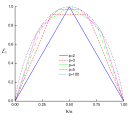
Figure 2: (color online) $\mathcal{E}_{1}$ as a function of $k$ for various values of the spacing $p$. The curve is always piecewise linear and weakly converges to $E_{1}$. Notice that for $k=\pi/2$ the entanglement is maximal whenever $p$ is even.

We next consider the case when $p=2$. The values $g_{2}(0)$ and $g_{2}(\pi)$ are given by

$$g_{2}(0) =\frac{1}{2}\bigl{(}g(0)+g(\pi)\bigr{)}=0$$ (29a)

and

$$g_{2}(\pi) =\frac{1}{2}\bigl{(}g(\pi/2)+g(3\pi/2)\bigr{)}=g(\pi/2).$$ (29b)

The latter is either $1$ or $-1$, and thus makes no contribution to entanglement. The critical angle is just $\theta^{\ast}=2k$ and hence we have $\mathcal{E}_{1}(2)=2Lk/\pi.$ The linear dependence on $k$ can be seen in Fig.2, where we plot the entanglement for various values of the spacing $p$. In the absence of any external magnetic field, i.e. for $k=\pi/2$, the entanglement attains its maximum possible value whenever $p$ is even. For larger values of $p$ the function is always piecewise linear, eventually converging to $E_{1}$.

It is important to observe that the expression (25) for the entanglement is continuous when we consider $p$ as a real number, despite the discontinuities that appear in (21). The function $g_{p}(0)$ is discontinuous whenever $pk=2n\pi$, but at those points $\theta^{\ast}$ vanishes and hence $\mathcal{E}_{1}(p)$ remains unaffected. On the other hand, $\mathcal{E}_{1}(p)$ is also oblivious to the jumps in the function $g_{p}(\pi)$, which occur at $pk=(2n+1)\pi$ (due to the variable $s$), because then we have $\theta^{\ast}=\pi$. Its derivative, on the other hand, is discontinuous: at the special points $pk=n\pi$ the entanglement has a local maximum with a cusp form. Remarkably, for a fixed $k$ its values at these maxima are all the same (i.e. they do not depend on $n$) and are equal to the large-$p$ limiting value,

$$\mathcal{E}_{1}(n\pi/k)=E_{1}.$$ (30)

In Fig.3 we plot $\mathcal{E}_{1}(p)$ as a function of the spacing for different values of the magnetic field $h=\cos k$. Since, of course, only integer values of $p$ may be realized in the actual chain, we take $k=\pi/\ell$, where $\ell$ is an integer. We see that this leads to the appearance of an unexpected length scale for the entanglement: it attains its maximal value whenever the spacing is a multiple of $\ell$. The existence of such a length scale appears to be a fundamental property of quantum spin chains in magnetic fields.

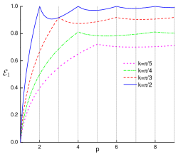
Figure 3: (color online) $\mathcal{E}_{1}$ as a function of the spacing $p$ for various values of the magnetic field $h=\cos k$. For $k=\pi/\ell$ there exists a typical length scale for the spacing: the entanglement is maximal for $p=n\ell$, and its value at these points is equal to the limit $E_{1}$.

Recently the formalism of Toeplitz determinants has been used to compute the ‘block’ entanglement of the more general XY model jpa38ari2005 , with finite anisotropy parameter $\gamma\neq 0$. The main difference with respect to the case $\gamma=0$ is the form of the function $g(\theta)$, which is no longer piecewise constant and becomes complex. Calculating the average (19) then becomes much less simple, but it is still possible to employ the present approach to obtain the entanglement for arbitrary values of the spacing $p$. A special case for which explicit calculations are possible is the Ising model without magnetic field, obtained from (1) by setting $\gamma=1$ and $h=0$. In this case we have $g(\theta)=e^{i\theta}$ and thus $g_{p}(\theta)=0$, leading to the result that $E_{\rm Ising}(L;p)=L$ for any value of $p$. This reflects the fact that the zero temperature ground state of this model is maximally entangled pra66tjo2002 .

IV Logarithmic correction

In order to obtain the logarithmic correction for the XX model we need to decompose the symbol (18) in the form

$$\lambda-g_{p}(\theta)=\phi(\lambda)t_{\beta}(\theta-\theta^{\ast})t_{-\beta}(\theta+\theta^{\ast}),$$ (31)

where

$$\phi(\lambda)=(\lambda-g_{p}(\pi))\left(\frac{\lambda-g_{p}(\pi)}{\lambda-g_{p}(0)}\right)^{-\theta^{\ast}/\pi}$$ (32)

is independent of $\theta$ and the discontinuities are accounted for by

$$t_{\beta}(\theta)=e^{-i\beta(\pi-\theta)},\quad\theta\in[0,2\pi).$$ (33)

The function $\beta(\lambda)$ is given by

$$\beta(\lambda)=\frac{-1}{2\pi i}\ln\left(\frac{\lambda-g_{p}(\pi)}{\lambda-g_{p}(0)}\right),$$ (34)

and the coefficient in the logarithmic correction to the entanglement is

$$\mathcal{E}_{2}(p)=\frac{1}{\pi i}\oint e(1,\lambda)\beta(\lambda)\frac{d\beta}{d\lambda}d\lambda.$$ (35)

Since for $p>1$ both $\left\lvert g_{p}(0)\right\rvert$ and $\lvert g_{p}(\pi)\rvert$ are smaller than unity, we can choose as our contour of integration the unit circle. Using power series expansions we arrive at

$$\mathcal{E}_{2}(p)=\frac{g_{p}(0)-g_{p}(\pi)}{2\pi^{2}\ln 2}I(g_{p}(0),g_{p}(\pi)),$$ (36)

where

$$I(a,b)=\sum_{m=0}^{\infty}\sum_{n=1}^{\infty}\sum_{j=1}^{n}\frac{a^{n}b^{m}-a^{m}b^{n}}{j(n+m+1)(n+m)}.$$ (37)

Since both $g_{p}(0)$ and $g_{p}(\pi)$ are piecewise constant as functions of $k$, the same is true for $\mathcal{E}_{2}$. In the left panel of Fig.4 we see that the number of jumps in this function grows as $p$ increases. On the other hand, for a given value of the magnetic field $\mathcal{E}_{2}$ decays rapidly as $p$ increases, and has discontinuities at $p=n\ell$ when $k=\pi/\ell$ (see the right panel of Fig.4). Notice that the vanishing of the logarithmic term in the entanglement is consistent with the fact that $E\rightarrow LE_{1}$ as $p\to\infty$ (cf. (28)).

Figure 4: Left: $\mathcal{E}_{2}$ as a function of $k$ for two values of the spacing. Right: $\mathcal{E}_{2}$ as a function of $p$ for two values of the magnetic field.

V Conclusions

In summary, we have extended the bipartite approach to entanglement in one-dimensional critical spin chains by introducing a new partition of the chain, the comb partition, which allows us to go beyond the simple ‘block’ picture and investigate non-local correlations analytically. The organizing subsystem consists of $L$ spins separated by $p$ sites, and we have found that as $p\rightarrow\infty$ its entanglement with the rest of the chain reduces to the sum of the individual contributions of its elements, although with a slow convergence rate that indicates the existence of long-range correlations. We have also found that the presence of a magnetic field induces a typical length scale for entanglement. It would be interesting the see if this length scale is present in other statistical properties of critical spin chains. Our results regarding a generalized version of the Emptiness Formation Probability, which has recently been computed for the XY model using Toeplitz determinants jpa38ff2005 , will appear elsewhere sepf .

We are grateful to Noah Linden for a stimulating discussion. MN thanks CAPES for financial support. JPK is supported by an EPSRC Senior Research Fellowship.

References

- (1) S. Sachdev, Quantum Phase Transitions, (Cambridge Univ. Press, Cambridge, 2000).
- (2) T.J. Osborne and M.A. Nielsen, Phys. Rev. A 66, 032110 (2002); Quantum. Inf. Process. 1, 45 (2002).
- (3) A. Osterloh et al., Nature 416, 608 (2002).
- (4) G. Vidal et al., Phys. Rev. Lett. 90, 227902 (2003).
- (5) J.I. Latorre, E. Rico and G. Vidal, Quant. Inf. and Comp. 4, 48 (2004).
- (6) V. Popkov and M. Salerno, Phys. Rev. A 71, 012301 (2005).
- (7) M.F. Yang, Phys. Rev. A 71, 030302(R) (2005); J. Eisert and M. Cramer, ibid 72, 042112 (2005); S.O. Skrovseth and K. Olaussen, ibid 72, 022318 (2005).
- (8) T.C. Wei et al., Phys. Rev. A 71, 060305(R) (2005); D. Bru et al., ibid 72, 014301 (2005); T.R. de Oliveira, G. Rigolin and M.C. de Oliveira, ibid 73, 010305 (2006).
- (9) C.H. Bennett et al., Phys. Rev. A 53, 2046 (1996).
- (10) W.K. Wootters, Phys. Rev. Lett. 80, 2245 (1998).
- (11) B.-Q. Jin and V.E. Korepin, J. Stat. Phys. 116, 79 (2004).
- (12) M.E. Fisher and R.E. Hartwig, Adv. Chem. Phys. 15, 333 (1968); E.L. Basor, Trans. Amer. Math. Soc. 239, 33 (1978); E.L. Basor and K.E. Morrison, Lin. Alg. App. 202, 129 (1994); T. Ehrhardt and B. Silbermann J. Funct. Anal. 148, 229 (1997).
- (13) V.E. Korepin, Phys. Rev. Lett. 92, 096402 (2004); P. Calabrese and J. Cardy, J. Stat. Mech. P06002 (2004).
- (14) J.P. Keating and F. Mezzadri, Commun. Math. Phys. 252, 543 (2004); Phys. Rev. Lett. 94, 050501 (2005).
- (15) M.M. Wolf, Phys. Rev. Lett. 96, 010404 (2006); D. Gioev and I. Klich, ibid 96, 100503 (2006).
- (16) M. Cramer and J. Eisert, quant-ph/0509167.
- (17) M.B. Plenio et al., Phys. Rev. Lett. 94, 060503 (2005); M. Cramer et al., Phys. Rev. A 73, 012309 (2006).
- (18) E. Baruch, M. McCoy and M. Dresden, Phys. Rev. A 2, 1075 (1970); E. Baruch and M. McCoy ibid 3, 786 (1971); ibid 3, 2137 (1971).
- (19) A.R. Its, B.-Q. Jin and V.E. Korepin, J. Phys. A 38, 2975 (2005).
- (20) M. Shiroishi, M. Takahashi and Y. Nishiyama, J. Phys. Soc. Japan 70, 3535 (2001); A.G. Abanov and F. Franchini, Phys. Lett. A 316, 342 (2003); F. Franchini and A.G. Abanov, J. Phys. A 38, 5069 (2005).
- (21) J.P. Keating, F. Mezzadri and M. Novaes, in preparation.