Quantum Dynamical Effects as a Singular Perturbation for Observables
in Open Quasi-Classical Nonlinear Mesoscopic Systems

Abstract

We review our results on a mathematical dynamical theory for observables for open many-body quantum nonlinear bosonic systems for a very general class of Hamiltonians. We show that non-quadratic (nonlinear) terms in a Hamiltonian provide a singular “quantum” perturbation for observables in some “mesoscopic” region of parameters. In particular, quantum effects result in secular terms in the dynamical evolution, that grow in time. We argue that even for open quantum nonlinear systems in the deep quasi-classical region, these quantum effects can survive after decoherence and relaxation processes take place. We demonstrate that these quantum effects in open quantum systems can be observed, for example, in the frequency Fourier spectrum of the dynamical observables, or in the corresponding spectral density of noise. Estimates are presented for Bose-Einstein condensates, low temperature mechanical resonators, and nonlinear optical systems prepared in large amplitude coherent states. In particular, we show that for Bose-Einstein condensate systems the characteristic time of deviation of quantum dynamics for observables from the corresponding classical dynamics coincides with the characteristic time-scale of the well-known quantum nonlinear effect of phase diffusion.

I Introduction

Real physical systems are not isolated, they are coupled to external degrees of freedom. The classical and quantum dynamics of these open systems are especially complex for nonlinear systems that exhibit several phenomena, including deviation of quantum dynamics from the corresponding classical one, quantum revivals, decoherence, and relaxation. Recently substantial effort has been devoted to study the open dynamics of nonlinear quantum systems, with the aim of understanding the quantum to classical transition in a controlled way nl

Standard mathematical treatments of open quantum nonlinear systems suffer from problems arising from the interplay between the nonlinearity and the openness of the system. Usually the dynamics of open quantum systems is studied using different mathematical approaches, such as the master equation for the reduced density matrix, which is an average of the full density matrix over the environment. Giulini ; ZurekRMP ; Paz2001 , and quasi-probability distributions (e.g. the so-called Q-function Gardiner2000 , the Wigner function Agarval1970 , etc). Although all of these approaches allow one, in principle, to calculate the time evolution of the average values of the dynamical variables of the system, they have significant drawbacks. In particular, these distribution functions may not be positively defined; they may be inconsistent for certain density matrices; it may be difficult to extract physical information from these distributions, especially in the context of quantum nonlinear open systems; in the “deep” quasi-classical region of parameters, $\epsilon=\hbar/J\ll 1$ (where $\hbar$ is Planck constant and $J$ is a characteristic action of the corresponding classical system) these quasi-probability distributions exhibit fast oscillations due to phases like $\exp(iS(t)/\hbar)$, with $|S(t)|\simeq J$. Therefore, it is difficult to separate the physical effects for dynamical observables (requiring an additional multi-dimensional integration of quasi-distribution densities) from the effects of errors related to a concrete mathematical approach.

We are approaching these problems using an alternative strategy that starts from a mathematical dynamical theory based on exact, linear partial differential equations (PDEs) for the observables of open many-body quantum nonlinear bosonic systems governed by a very general class of Hamiltonians (see Berman1994 ; Berman2004 ; Dalvit2006 and references therein). The key advantage of this method is that it leads to a well-behaved asymptotic theory for open quantum systems in the quasi-classical region of parameters. This approach is a generalization to the open case of the asymptotic theory for bosonic and spin closed quantum systems Berman1994 ; Vishik2003 ; Berman2003 , and it can be applied to general open quantum nonlinear bosonic and spin systems for a large range of parameters, including the deep quasi-classical region.

We concentrate our attention on a discussion of the method which can be used to observe quantum effects after decoherence and relaxation, in the deep quasi-classical region of parameters. We argue that one can use for these purposes a Fourier spectrum of the dynamical observables, since its width contains characteristic information of such quantum effects. Our observation is based on our first studies Dalvit2006 ; Berman2004 of this new approach to quantum nonlinear systems interacting with an environment. As will be discussed below, certain quantum effects which are presented in the dynamics of these nonlinear systems are robust to the influence of the environment, and survive after decoherence and relaxation processes take place. In order to observe these effects experimentally it is necessary to have a quasi-classical system in certain region of parameters. We call these systems “mesoscopic”, mainly because the parameter $\epsilon$ should not be too small. In this sense, many quasi-classical systems have the drawback that they are either “too classical” (i.e., they have a large $J$ so that the quasi-classical parameter $\epsilon$ is extremely small), or they interact too strongly with the environment, or their effective temperature is so high that quantum effects that we are talking about are washed out. Only recently have adequate open nonlinear quasi-classical systems become available, including Bose-Einstein condensates (BEC) with large number of atoms and thermally well isolated; high frequency cantilevers with large nonlinearities and at sufficiently low temperatures; and nonlinear optical systems in high Q resonators, among others. We present estimates on the parameter regions where survival of certain quantum effects to environment-induced decoherence can be observed in these systems.

II Dynamics of quantum observables for closed quantum nonlinear systems

We first consider closed quantum nonlinear systems. As a simple example we take the one-dimensional quantum nonlinear oscillator (QNO) described by the Hamiltonian BermIomiZasl1 ; Berman1994 (see also an application of this Hamiltonian for the BEC system in Section V)

$$H_{s}=\hbar\omega a^{\dagger}a+\mu\hbar^{2}(a^{\dagger}a)^{2}\;,\ [a^{\dagger},a]=1,$$ (1)

where $a,a^{\dagger}$ are the annihilation and creation operators, $\omega$ is the frequency of linear oscillations, and $\mu$ is a dimensional parameter of nonlinearity. We assume that initially the QNO is prepared in a coherent state $|\alpha\rangle\;(a|\alpha\rangle=\alpha|\alpha\rangle$). In the classical limit ($a\rightarrow\alpha,a^{\dagger}\rightarrow\alpha^{*},|\alpha|^{2}\rightarrow\infty,\hbar|\alpha|^{2}=J$, the classical action of the linear oscillator) the Hamiltonian (1) becomes $H_{\rm cl}=\omega J+\mu J^{2}$. Below we use the following dimensionless notation: $\tau\equiv\omega t$, $\bar{\mu}\equiv\hbar\mu/\omega$, and $\mu_{\rm cl}\equiv\mu J/\omega$. The quantum parameter of nonlinearity $\bar{\mu}$ can be presented as the product of two parameters, quantum and classical, $\bar{\mu}=\epsilon\mu_{\rm cl}$. The parameter $\mu_{\rm cl}$ characterizes the nonlinearity in the classical nonlinear oscillator (BEC, cantilever, optical field, etc) and can be written as $\mu_{\rm cl}=(J/2\omega)(d\omega_{\rm cl}/dJ$), where $\omega_{\rm cl}=dH_{\rm cl}/dJ=\omega+2\mu J$ is the classical frequency of nonlinear oscillations. The limit $\mu_{\rm cl}\ll 1$ corresponds to weak nonlinearity, while $\mu_{\rm cl}\simeq 1$ corresponds to strong nonlinearity. As was mentioned above, $\epsilon$ is the quasi-classical parameter. Namely, $\epsilon\simeq 1$ corresponds to the pure quantum system, and $\epsilon\ll 1$ corresponds to the quasi-classical limit, which is the subject of our interest.

II.1 Closed partial differential equation for observables

A closed linear PDE which describes the time evolution of the expectation value of any observable of the system can be easily derived when the system is initially populated in a coherent state $|\alpha\rangle$ (see Berman1994 and references therein). Namely, for an arbitrary operator function $f=f(a,a^{\dagger})$, the time-dependent expectation value (observable) of such a function,

$$f(\alpha^{*},\alpha,\tau)=\langle\alpha|e^{iHt/\hbar}fe^{-iHt/\hbar}|\alpha\rangle,$$ (2)

satisfies a PDE of the form

$$\partial f/\partial\tau=\hat{K}f,$$ (3)

where$\hat{K}=\hat{K}_{\rm cl}+\epsilon\mu_{\rm cl}\hat{K}_{\rm q}$. Here the operator $\hat{K}_{\rm cl}$ includes only the first order derivatives and describes the corresponding classical limit, while the operator $\hat{K}_{\rm q}$ includes higher-order derivatives and contains the quantum effects. For the Hamiltonian (1) we have

$$\frac{\partial f}{\partial\tau} = i(1+\bar{\mu}+2\bar{\mu}|\alpha|^{2})\left(\alpha^{*}\frac{\partial}{\partial\alpha^{*}}-\alpha\frac{\partial}{\partial\alpha}\right)$$ (4)

$$+i\bar{\mu}\left((\alpha^{*})^{2}\frac{\partial^{2}}{\partial(\alpha^{*})^{2}}-\alpha^{2}\frac{\partial^{2}}{\partial\alpha^{2}}\right)f.$$

In particular, for the operator function $f(\tau=0)=a$, the evolution of $f(\tau)$ corresponds to the evolution of $\alpha(\tau)=\langle\alpha|a(\tau)|\alpha\rangle$, with the initial condition $\alpha(\tau=0)=\alpha$. In this case Eq. (4) can be solved exactly Berman1994 ; BermIomiZasl1

$$\alpha(\tau)=\alpha\,e^{-i(1+\bar{\mu})\tau}\;e^{|\alpha|^{2}(e^{-2i\bar{\mu}\tau}-1)}.$$ (5)

Fig. 1 depicts the dynamics described by the observable in Eq. (5) in the coordinate-momentum plane. The effective coordinate is defined as $x(\tau)=(\alpha^{*}(\tau)+\alpha(\tau))/\sqrt{2}$, and the effective momentum is defined as $p(\tau)=i(\alpha^{*}(\tau)-\alpha(\tau))/\sqrt{2}$. The corresponding classical dynamics is described by the function $\alpha_{\rm cl}(\tau)=\alpha e^{-i(1+2\mu_{\rm cl})\tau}$, which corresponds to the circumference in Fig. 1. Note that Eq. (4) maintains its form for any observable $f$, but the initial conditions for different observables are different. This is also the case for any quantum nonlinear Hamiltonian with many degrees of freedom.

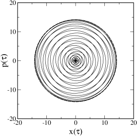
Figure 1: Quasi-classical dynamics as described by the observable in Eq. (5). Parameters are $\epsilon=0.02$, $\bar{\mu}=0.01$, $\tau_{\hbar}=5$, $\tau_{\rm R}=314$, $\tau_{\rm cl}=2.09$, $|\alpha|^{2}=100$, $\mu_{\rm cl}=1$. Hence $\tau_{\rm cl}<\tau_{\hbar}<\tau_{\rm R}$.

II.2 Characteristic time-scales for a closed quantum nonlinear system

The solution (5) has three characteristic time-scales BermIomiZasl1 ; Berman1994 ; Berman2002 ; Pit1 . In the limit $\bar{\mu}\tau\ll 1$, it can be re-written in the form

$$\alpha(\tau)=\alpha_{\rm cl}(\tau)e^{-\tau^{2}/2\tau_{\hbar}^{2}}\;\left[1+O(\bar{\mu}\tau)+O(|\alpha|^{2}\bar{\mu}^{3}\tau^{3})\right].$$ (6)

The first time-scale is the characteristic classical time-scale, which can be chosen as the period of classical nonlinear oscillations,

$$\tau_{\rm cl}=\frac{2\pi\omega}{\omega_{\rm cl}}=\frac{2\pi}{1+2\mu_{\rm cl}}.$$ (7)

The second time-scale is a characteristic time of departure of the quantum dynamics from the corresponding classical one

$$\tau_{\hbar}=\frac{1}{2\bar{\mu}|\alpha|}.$$ (8)

This time-scale characterizes the departure of quantum dynamics from the classical one for classically stable systems. Historically, this time-scale was introduced for classically unstable (classically chaotic) systems in Berman1978 , and it was shown to have a logarithmic dependence on $\epsilon$ (see also Chirikov1991 ; Chirikov1988 ). The time-scale $\tau_{\hbar}$ is usually called the Ehrenfest time. The amplitudes of quantum and classical observables coincide at multiple times of the quantum recurrence time-scale, which is the third characteristic time-scale,

$$\tau_{\rm R}=\frac{\pi}{\bar{\mu}}.$$ (9)

Since we are interested in the quasi-classical region of parameters, it is reasonable to impose the following inequalities on these three characteristic time-scales: $\tau_{\rm cl}<\tau_{\hbar}\ll\tau_{\rm R}$. In our case, $\tau_{\rm cl}/\tau_{\hbar}=4\pi\bar{\mu}|\alpha|/(1+2\mu_{\rm cl})\approx\pi\sqrt{\epsilon}\ll 1$, and $\tau_{\hbar}/\tau_{\rm R}\approx\sqrt{\epsilon}/\pi\ll 1$. When deriving the first inequality, we used the conditions $|\alpha|^{2}\simeq J/\hbar=1/\epsilon$ and $\mu_{\rm cl}\simeq 1$, which corresponds to the condition of strong nonlinearity. Note that the condition $|\alpha|^{2}\bar{\mu}^{3}\tau^{3}\simeq 1$ (see the third term in (6) in the square brackets in the expression for $\alpha(\tau)$) gives the characteristic times $\tau\gg\tau_{\hbar}$, namely $\tau/\tau_{\hbar}=2/\epsilon^{1/6}\gg 1$. This means that the third term in Eq. (6) is small on the time scale $\tau_{\hbar}$. For the values of parameters in Fig. 1 the inequalities $\tau_{\rm cl}<\tau_{\hbar}\ll\tau_{\rm R}$ are satisfied.

II.3 Quantum effects as a singular perturbation to the classical solution

As was mentioned above, the form of the differential operator $\hat{K}$ is

$$\hat{K}=\hat{K}_{\rm cl}+\epsilon\mu_{\rm cl}\hat{K}_{\rm q}.$$

The operator $\hat{K}_{\rm cl}$ includes only the first order derivatives and describes the classical dynamics of the system. Usually, the corresponding classical solution can be found by the method of characteristics, or some alternative well-developed methods. Note that even this part of the solution can be rather complicated, especially for classically unstable and chaotic systems, and usually requires large-scale numerical simulations. (See details for closed quantum nonlinear systems and quantum nonlinear systems interacting with the time-periodic fields Berman1994 .) Another example which demonstrates the application of the approach based on PDEs with the operator $\hat{K}$ is considered in Berman2002 for a unstable quantum nonlinear system describing the dynamics of a Bose-Einstein condensate with attractive interactions.

For quantum linear systems ($\mu_{\rm cl}=0$) the quantum effects vanish for any values of the quasi-classical parameter $\epsilon$. The differential operator $\hat{K}_{\rm q}$ includes second and higher order derivatives, and it describes quantum effects. The solutions of these PDEs are well behaved in the quasi-classical region, $\epsilon\ll 1$, and in contrast to the fast oscillating WKB solutions (typical of standard methods based on quasi-probability distributions), our method leads to the so-called Laplace-type expansions Vishik2003 . The crucial property of the Laplace asymptotics is that the dynamical observables are exponentially localized in phase space around coherent states.

Quantum effects for observables represent a singular perturbation to the classical solution. Indeed, in the quasi-classical region, quantum terms in the PDEs are represented by the product of the small parameter $\epsilon$ times high order derivatives. Consequently, these quantum terms lead to a secular behavior of the solution, which diverges in time from the corresponding classical solution. Only the case $\epsilon=0$ (for finite $\mu_{\rm cl}$) corresponds to the exact classical limit. But the problem with this limit is that for any real system $\epsilon\neq 0$ (because $\hbar\neq 0$ and $J\neq\infty$). Then, even a very small value of $\epsilon$ still “mathematically” results in a singular perturbation to the classical solution due to the quantum terms.

The singularity arising from the quantum terms reminds, up to some extent, of the singularity provided by a “small” viscosity in the Navier-Stokes (NS) equation, describing the dynamics of liquid and gas flows. Indeed, in the NS equation a small viscosity multiplies the higher order spatial derivatives. Then, even for very large Reynolds numbers (when the nonlinear terms are very large compared to the viscous ones), the viscosity plays a crucial role in the dynamics of the flow, even though it formally represents a “small” perturbation. Similarly, in the quantum case the small parameter $\epsilon$ multiplies the higher order derivatives, which results in a quantum singular perturbation for observables even in the “deep” quasi-classical region. It is this singularity that leads to a significant difference from the classical solution.

II.4 Frequency Fourier spectrum for quantum observables

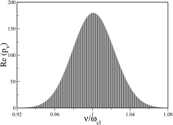
Figure 2: Frequency spectrum of the effective momentum $p(\tau)$. Parameters are $\epsilon=1/900$, $\bar{\mu}=1/900$, $\tau_{\hbar}\approx 15$, $\tau_{\rm R}\approx 900\pi$, $\tau_{\rm cl}\approx 2\pi/3$, and $|\alpha|^{2}=900$. Hence $\tau_{\rm cl}<\tau_{\hbar}\ll\tau_{\rm R}$.

The observable $\alpha(\tau)$ can be written in the form

$$\alpha(\tau)=\alpha e^{-i(1+\bar{\mu})\tau-i|\alpha|^{2}\sin(2\bar{\mu}\tau)}\;e^{-2|\alpha|^{2}\sin^{2}(\bar{\mu}\tau)}.$$ (10)

The first exponent in Eq. (10) is responsible for phase modulations of the classical dynamics, while the second one is responsible for amplitude modulations. The characteristic time-scale of the amplitude modulations, $\tau_{\rm am}$, is defined by the condition $|\alpha|^{2}\bar{\mu}^{2}\tau_{\rm am}^{2}\approx 1$, or by the time-scale $\tau_{\rm am}\approx\tau_{\hbar}$. The time-scale of phase modulations of the classical dynamics is defined by the condition $|\alpha|^{2}\bar{\mu}\tau_{\rm ph}\approx 1$, or $\tau_{\rm ph}\approx\tau_{\hbar}/\sqrt{\epsilon}\gg\tau_{\hbar}$. Thus, the shortest time-scale which characterizes the deviation of the quantum dynamics from the corresponding classical one is the time $\tau_{\hbar}$. Moreover, this time-scale is responsible for the finite width of the spectral line $\Delta\nu_{\hbar}\approx 2\sqrt{2}/\tau_{\hbar}$.

Fig. 2 depicts the frequency Fourier spectrum of the effective momentum $p(\tau)$, with initial condition $p(0)=0$. One can see that the frequency spectrum consists of one central line with $\nu=\omega_{\rm cl}=1+2\mu_{\rm cl}$, and a width which is approximately equal to $\Delta\nu\approx\Delta\nu_{\hbar}$. In our case the analytical estimate gives $\Delta\nu_{\hbar}\approx 2\sqrt{2}/\tau_{\hbar}\approx 0.19$, which is very close to the numerical results presented in Fig. 2, $\Delta\nu\approx 0.183$. The fine structure of the frequency spectrum is provided by the characteristic revival time scale $\tau_{\rm R}=\pi/\bar{\mu}$, or by the frequencies $\nu_{n}=2\bar{\mu}n$, which are responsible for the complicated dynamics of quantum recurrences.

III Dynamics of quantum observables for open quantum nonlinear systems

The Hamiltonian of open quantum nonlinear system interacting with an environment contains three terms,

$$\hat{H}=\hat{H}_{\rm S}+\hat{H}_{\cal E}+\hat{H}_{\rm int}.$$ (11)

The first term is typically a time-independent polynomial Hamiltonian of a general form which describes the self evolution of the closed system,

$$\hat{H}_{\rm S}=\sum_{l,s}H_{l,s}a^{\dagger l_{1}}_{1}\ldots a^{\dagger l_{N}}_{N}a^{s_{1}}_{1}\ldots a^{s_{N}}_{N},$$

where $H_{l,s}=H^{*}_{l,s}$, $l=(l_{1},\ldots,l_{N})\in Z^{N}_{+}$, and $s=(s_{1},\ldots,s_{N})\in Z^{N}_{+}.$ The operators $a_{l}$ and $a^{\dagger}_{k}$ satisfy bosonic commutation relations, $[a_{l},a^{\dagger}_{k}]=\delta_{l,k}$. A particular system corresponds to a particular choice of the coefficients $H_{l,s}$ in $\hat{H}_{\rm S}$. The second term is the Hamiltonian of the environment, which, for example, can be modeled by a collection of harmonic oscillators,

$$\hat{H}_{\cal E}=\sum_{\vec{q}}\hbar\omega_{\vec{q}}\,b^{\dagger}_{\vec{q}}\,b_{\vec{q}}.$$ (12)

Usually the oscillators of the environment are assumed to be initially in thermal equilibrium,

$$\rho_{\cal E}(t=0)=Z_{\cal E}^{-1}e^{-\hat{H}_{\cal E}/k_{\rm B}T},$$

where $Z_{\cal E}={\rm Tr}[e^{-\hat{H}_{\cal E}/k_{\rm B}T}]$ is the partition function of the environment, $T$ is the temperature of the environment, and $k_{\rm B}$ is Boltzmann constant. The third term is the interaction Hamiltonian between the system and the environment. Prototype examples are the dipole-dipole interaction Hamiltonian,

$$\hat{H}_{\rm int}=\hbar\sum_{n,{\vec{q}}}\lambda_{n,{\vec{q}}}[(a^{\dagger}_{n}+a_{n})(b^{\dagger}_{\vec{q}}+b_{\vec{q}})],$$ (13)

and the density-density interaction Hamiltonian

$$\hat{H}_{\rm int}=\hbar^{2}a^{\dagger}a\sum_{\vec{q}}\lambda_{\vec{q}}\,b^{\dagger}_{\vec{q}}\,b_{\vec{q}}.$$ (14)

III.1 The differential operator $\hat{K}$ for many-body systems

In a general many-body system the differential operator $\hat{K}$ can formally be written as

$$\hat{K} = \frac{i}{\hbar}e^{-\sum(|\alpha_{n}|^{2}+|\beta_{\vec{q}}|^{2})}\sum\left[H\left(\alpha^{*}_{l},\beta^{*}_{q},\frac{\partial}{\partial\alpha^{*}_{l}},\frac{\partial}{\partial\beta^{*}_{q}}\right)\right.$$ (15)

$$\left.-H\left(\alpha_{l},\beta_{q},\frac{\partial}{\partial\alpha_{l}},\frac{\partial}{\partial\beta_{q}}\right)\right]\;e^{-\sum(|\alpha_{n}|^{2}+|\beta_{\vec{q}}|^{2})}.$$

Note that after explicit differentiations, exponents in $\hat{K}$ vanish. Specific examples considered in our previous works include: (i) a closed quantum one-dimensional nonlinear system in the vicinity of an elliptic Berman1994 ; Berman2003 or a hyperbolic Berman2003 ; Berman2002 point; (ii) chaotic systems describing the interaction of atoms with radiation and external radio frequency fields Berman1994 ; and (iii) the quantum Brownian motion problem for a nonlinear system oscillator Dalvit2006 ; Berman2004 .

III.2 Frequency Fourier spectrum of $p(\tau)$ in the presence of an environment

Let us introduce formally a relaxation (dissipation) term into Eq. (5). Namely, we consider the function

$$\alpha(\tau)=\alpha\,e^{-\gamma\tau-i(1+\bar{\mu})\tau}\;e^{|\alpha|^{2}(e^{-2i\bar{\mu}\tau}-1)},$$ (16)

where the parameter $\gamma$ plays the role of an effective relaxation. The characteristic time scale of relaxation is $\tau_{\gamma}=1/\gamma$. We consider the frequency Fourier spectrum of the momentum $p(\tau)=i(\alpha^{*}(\tau)-\alpha(\tau))/\sqrt{2},$ with $\alpha(\tau)$ given by Eq. (16), for two cases: (i) $\tau_{\gamma}\gg\tau_{\hbar}$ (Fig. 3a), and (ii) $\tau_{\gamma}<\tau_{\hbar}$ (Fig. 3b) (similar dependencies can be built for the effective coordinate $x(\tau)$). As one can see, when the influence of the effective dissipation is small (Fig. 3a), the width of the Gaussian spectral line (at the level $e^{-1}$) is still determined by the time-scale $\tau_{\hbar}$ ($\Delta\nu_{\hbar}\simeq 2\sqrt{2}/\tau_{\hbar}\approx 0.19$), and not by the environment ($\Delta\nu_{\gamma}\simeq 2\gamma=0.001$). The numerical results give $\Delta\nu\approx 0.186$. Note that in this case the fine structure of the spectral line is not completely destroyed, as both time-scales, $\tau_{\rm R}\approx 2826$ and $\tau_{\gamma}=2000$, are of the same order. In the case of strong dissipation (Fig. 3b), the width of the spectral line has a Lorentzian form,

$${\rm Re}(p_{\nu})=\gamma^{2}{\rm Re}(p_{0})/(\gamma^{2}+\nu^{2}),$$

with a width (at ${\rm Re}(p_{\nu})=1/2$) determined by the dissipation parameter $\gamma$ ($\Delta\nu_{\gamma}\approx 2\gamma=1$). The numerical results are in good agreement, $\Delta\nu\approx 1$. Also, the fine structure is destroyed, as in this case $\tau_{\gamma}=2\ll\tau_{\rm R}\approx 2826$. In Berman2004 we studied the concrete example of the QNO interacting with an environment in which both relaxation and decoherence take place, and we found that the frequency spectrum behaves in a similar way as the toy model discussed in this subsection.

III.3 Characteristic parameters for observation of quantum effects after decoherence and relaxation

As was discussed above, for the simple closed quantum nonlinear system given by Eq. (1) there are three characteristic time-scales (see Vishik2003 for details on multi-dimensional systems). Due to the interaction with the environment, two new time-scales appear: $\tau_{\rm d}$ - a very short decoherence time, and $\tau_{\gamma}$ -the relaxation time. All of these five time-scales depend on the parameters of the system and the environment. The typical region of parameters in which one can observe quantum effects after decoherence and relaxation is $\tau_{\rm d}\ll\tau_{\rm cl}<\tau_{\hbar}<\tau_{\gamma}<\tau_{\rm R}$. In the following we will consider a system which satisfies this region of parameter a “quasi-classical nonlinear mesoscopic system”. The key inequality is $\tau_{\hbar}<\tau_{\gamma}$. In this case, the deviation of the quantum dynamics from the classical one formally works as an effective “quantum relaxation” (or a “quantum amplitude modulation”), which gives the main contribution to the frequency spectral line width. The relations between $\tau_{\rm cl}$ and $\tau_{\hbar}$ , and between $\tau_{\rm R}$ and $\tau_{\gamma}$ are not so important. There can be additional time-scales related to accumulation of quantum phases Berman2004 , multi-dimensionality Vishik2003 , etc. The details for a one-dimensional case were presented in Dalvit2006 ; Berman2004 .

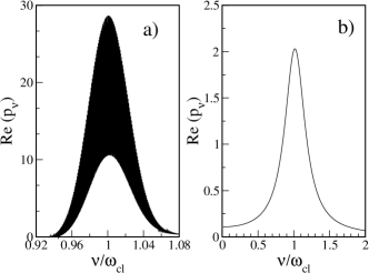
Figure 3: Fourier frequency spectrum of the momentum $p(\tau)$ obtained from Eq. (16). Parameters are: a) $\gamma=0.0005$, $\tau_{\gamma}=2000\gg\tau_{\rm\hbar}\approx 15$; b) $\gamma=0.5$, $\tau_{\gamma}=2<\tau_{\hbar}\approx 15$; all other parameters are the same as in Fig. 2.

IV An exact solvable example of an open quantum nonlinear system

IV.1 Phase decoherence

Although the PDEs described above look rather complicated, especially for open quantum nonlinear systems, we have found the exact solution for a quantum nonlinear oscillator interacting with the environment in the special case of a density-density type of interaction, as in Eq.(14). The type of interaction does not provide relaxation processes through energy exchange between the QNO and the environment, but leads to phase decoherence. These effects result in the decay of the amplitude of oscillations of the QNO (similar to the effects of relaxation), and survive in the classical limit, where they correspond to the dephasing of the QNO.

We summarize here the results of Dalvit2006 in the context of the quantum-classical transition for observables and the frequency Fourier spectrum. We choose the system Hamiltonian $\hat{H}_{\rm S}$ as in Eq. (1), the environment Hamiltonian $\hat{H}_{\cal E}$ as in Eq. (12), and a density-density interaction Hamiltonian $\hat{H}_{\rm int}$ as in Eq. (14). For the model under consideration, the interaction with the environment introduces a single time scale, $\tau_{\rm d}$ , which plays the role of a decoherence time. This time-scale is not small, and survives even in the classical limit: $|\alpha|^{2}\rightarrow\infty$, $|\beta_{\vec{q}}|^{2}\rightarrow\infty$, $\hbar\rightarrow 0$, $\hbar|\alpha|^{2}=J=const$, $\hbar|\beta_{\vec{q}}|^{2}=J_{\vec{q}}=const$, $\lambda_{\vec{q}}=const$. The typical region of parameters in which one can observe quantum effects is $\tau_{\rm cl}<\tau_{\hbar}<\tau_{\rm d}<\tau_{\rm R}$. The key inequality is now $\tau_{\hbar}<\tau_{d}$. In this case, the deviation of the quantum dynamics from the classical one formally works as an effective “quantum relaxation” (or a “quantum amplitude modulation”), which gives the main contribution to the frequency spectral line width. The relations between $\tau_{\rm cl}$ and $\tau_{\hbar}$ , and between $\tau_{\rm R}$ and $\tau_{d}$ are not so important.

Although this model is rather trivial because the full Hamiltonian can be diagonalized in the number basis for the joint system-environment Hilbert space, it is a useful model system for the purposes of demonstration of our approach. Following our previous results Dalvit2006 it is possible to write an exact linear PDE for any quantum dynamical observable in the joint Hilbert space

$$f(\alpha^{*},\alpha;\beta^{*}_{\vec{q}},\beta_{\vec{q}};t)=\langle\alpha,\beta_{\vec{q}}|\hat{f}(t)|\alpha,\beta_{\vec{q}}\rangle,$$ (17)

where $\hat{f}(t)=f(a^{\dagger}(t),a(t);b^{\dagger}_{\vec{q}}(t),b_{\vec{q}}(t))$ is a generic Heisenberg operator function, and $|\alpha,\beta_{\vec{q}}\rangle=|\alpha\rangle\prod_{j}|\beta_{\vec{q}_{j}}\rangle$ is an initial coherent state of the system and the environment. Here $a^{\dagger}(t)$, $a(t)$, $b^{\dagger}_{\vec{q}}(t)$, and $b_{\vec{q}}(t)$ are the Heisenberg bosonic creation and annihilation operators for the system and the environment, respectively, and $\vec{q}=(\vec{q}_{1},\vec{q}_{2},\ldots)$. The corresponding PDE has the form

$$\frac{\partial}{\partial t}f(\alpha^{*},\alpha;\beta^{*}_{\vec{q}},\beta_{\vec{q}})=\hat{K}f(\alpha^{*},\alpha;\beta^{*}_{\vec{q}},\beta_{\vec{q}};t),$$ (18)

where the differential operator $\hat{K}$ includes the derivatives of different orders over $\alpha^{*}$, $\alpha$, $\beta^{*}_{\vec{q}}$ and $\beta_{\vec{q}}$, and depends on the explicit form of the corresponding full Hamiltonian. As before, the general form of the differential operator $\hat{K}$ is $\hat{K}=\hat{K}_{\rm cl}+\hat{K}_{\rm q}$. The operator $\hat{K}_{\rm cl}$ includes only the first order derivatives and describes the classical dynamics of the system and environment. The operator $\hat{K}_{\rm q}$ describes the quantum effects of the system and the environment. The explicit expressions for both these operators are given in Dalvit2006 .

In order to study the reduced dynamics of the system, the function $f(\alpha^{*},\alpha;\beta^{*}_{\vec{q}},\beta_{\vec{q}})$ has to be traced over the variables of the environment $\beta^{*}_{\vec{q}},\beta_{\vec{q}}$. We have assumed above that initially each environmental oscillator is populated initially in the coherent state $|\beta_{\vec{q}}\rangle$. Let us now assume that the each environmental oscillator is initially in a mixed thermal state at temperature $T$. Then we should perform an additional averaging of the environmental oscillators over the thermal distribution. The corresponding procedure is thoroughly explained in Dalvit2006 . The exact solution for the system observable $\langle\alpha(\tau)\rangle_{\cal E}$, averaged over the environmental variables, is

$$\langle\alpha(\tau)\rangle_{\cal E}=\alpha(\tau)R(\tau),$$ (19)

where $\alpha(\tau)$ is defined in Eq. (3), and

$$R(\tau) = \prod_{\vec{q}}R^{(\vec{q})}(\tau),$$

$$R^{(\vec{q})}(\tau) = \frac{1-e^{-\hbar\omega_{\vec{q}}/k_{B}T}}{1-e^{-\hbar\omega_{\vec{q}}/k_{B}T-i\hbar\lambda_{\vec{q}}\tau/\omega}}.$$ (20)

IV.2 Classical limit

Let us write the complex quantity $R^{(\vec{q})}(\tau)$ in terms of its modulus and phase, $R^{(\vec{q})}(\tau)=e^{i\varphi^{(\vec{q})}(\tau)}|R^{(\vec{q})}(\tau)|$. Then, we have from Eq.(20)

$$|R(\tau)| = e^{-\Gamma(\tau)},$$

$$\Gamma(\tau) = -\frac{V}{2\pi^{2}}\int_{0}^{\infty}dq\,q^{2}\ln(|R^{(q)}(\tau)|),$$ (21)

where $V$ is the volume of the thermal bath. In the classical limit ($\hbar\rightarrow 0$) we have for $\Gamma(\tau)$

$$\Gamma(\tau)\approx\frac{\tau^{2}}{2\tau_{d}^{2}},~{}~{}\frac{1}{\tau_{d}^{2}}=\frac{V}{2\pi^{2}}\frac{(k_{B}T)^{2}}{\omega^{2}}\int_{0}^{\infty}dq{{q^{2}\lambda^{2}_{{\vec{q}}}}\over{\omega_{\vec{q}}^{2}}},$$ (22)

and the phase $\varphi^{({\vec{q}})}(\tau)$ is

$$\varphi^{(\vec{q})}(\tau)\approx-{{\lambda_{\vec{q}}k_{B}T}\over{\omega_{\vec{q}}\,\omega}}\tau.$$ (23)

The function $\alpha(\tau)$ in Eq. (19) coincides with that in Eq. (5). It is clear from Eq. (19) that under the condition

$$\tau_{\hbar}\ll\tau_{d},$$ (24)

the width of the frequency spectrum of $\langle\alpha(\tau)\rangle_{\cal E}$ is defined by the time-scale, $\tau_{\hbar}$, and not by the interaction with the environment. In the opposite case, $\tau_{\hbar}\gg\tau_{d}$, the width of the spectral line is determined by the interaction with the environment. A similar result was obtained in Berman2004 for the QNO interacting via the dipole-dipole interaction with the environment Eq.(13). But in the latter case, the time-scale $\tau_{d}$ in Eq. (24) should be substituted by the relaxation time $\tau_{\gamma}$.

V Estimates for concrete systems

Our main statement is that generally there is no classical limit for the dynamics of quantum nonlinear systems interacting with the environment, even when these systems are in the deep quasi-classical region of parameters. The corresponding systems were called above quasi-classical nonlinear mesoscopic systems (QCNMS). In this context we note that most classical systems surrounding us represent a very particular exception due to (i) either an extremely deep quasi-classicality (extremely small value of $\epsilon$) and/or (ii) a very strong interaction with the environment. At the same time, the general belief in the recent scientific literature is that after the process of decoherence, the quasi-classical system can be described by using classical probabilistic approaches. According to the results discussed here it appears to be true only (i) for quantum linear systems (with quadratic Hamiltonians) or (ii) for quantum nonlinear systems with significantly small value of a quasi-classical parameter $\epsilon$. For the QCNMS quantum effects survive after the processes of decoherence and relaxation took place. Moreover, these quantum effects make a crucial contribution to the dynamics of observables. This observation may have significant relevance for the understanding of the properties of noise in complex quantum systems and nanodevices. In particular, the performance of future BEC based interferometers and nano machines will be limited by the level of noise.

The key condition for survival of quantum effects for observables related to the time-scale $\tau_{\hbar}$ is $\tau_{\hbar}<\tau_{\gamma}$, which, in the simplest case of the quantum nonlinear oscillator can be written in the form

$$\Theta\equiv\frac{\tau_{\gamma}}{\tau_{\hbar}}=2\mu_{\rm cl}\sqrt{\epsilon}\tau_{\gamma}\gg 1.$$ (25)

We now present estimates for different real QCNMS that may satisfy the above condition, and therefore may lead to the observation of certain quantum effects that survive the process of environment-induced decoherence and dissipation.

V.1 Bose-Einstein condensates in a one-dimensional toroidal geometry

We start with a one-dimensional BEC confined in a toroidal geometry, and described by the quantum field equation (see Berman2002 ; weibin , and references therein)

$$i{{\partial\hat{\Psi}}\over{\partial\tau}}=\Bigg{[}-{{\partial^{2}}\over{\partial\theta^{2}}}+2\pi\varepsilon\hat{\Psi}^{\dagger}\hat{\Psi}\Bigg{]}\hat{\Psi}.$$ (26)

Here $\varepsilon=4Ra/S$, $R$ is the radius of the toroidal trap, $S$ is the area of the cross-section of the torus, and $a$ the interatomic s-wave scattering length ($a>0$ for a repulsive interaction, and $a<0$ for an attractive interaction). The dimensionless time is $\tau=\hbar t/2mR^{2}$. The operator $\hat{\Psi}(\theta,\tau)$ can be expanded as

$$\hat{\Psi}(\theta,\tau)={{1}\over{\sqrt{2\pi}}}\sum_{k=-\infty}^{\infty}\hat{a}_{k}(\tau)e^{ik\theta}.$$ (27)

Here $\hat{a}_{k}(\tau)$ and $\hat{a}_{k}^{\dagger}(\tau)$ are annihilation and creation bosonic operators, respectively, and the field operator is periodic $\hat{\Psi}(\theta+2\pi,\tau)=\hat{\Psi}(\theta,\tau)$ and satisfies the normalization condition

$$\int_{0}^{2\pi}\hat{\Psi}^{\dagger}(\theta,\tau)\hat{\Psi}(\theta,\tau)d\theta=\sum_{k=-\infty}^{\infty}\hat{n}_{k}\equiv\hat{N},$$ (28)

where $\hat{n}_{k}$ is the operator of the number of particles in the mode with momentum $k$, and $\hat{N}$ is the operator of the total number of particles.

In the following we only consider the case of repulsive interactions, $a>0$. ¿From Eqs. (26) and (27) it follows that the operators $\hat{a}_{k}(\tau)$ satisfy the following system of coupled first-order differential equations:

$$i\dot{\hat{a}}_{k}=k^{2}\hat{a}_{k}+\varepsilon\sum_{k_{1},k_{2},k_{3}=-\infty}^{\infty}\hat{a}_{k_{1}}^{\dagger}\hat{a}_{k_{2}}\hat{a}_{k_{3}}\delta_{k+k_{1}-k_{2}-k_{3},0},$$ (29)

where “dot” means derivative with respect to $\tau$. Here we shall limit ourselves to consider only a single mode in Eq.(29): $\hat{a}_{k}^{\prime}=\hat{a}_{k}\delta_{k^{\prime},k}$, which is stable under the condition $a>0$ (For a more general case see (bikt1 ; bt )). In this simplified case Eq. (29) takes the form

$$i\dot{\hat{a}}_{k}=k^{2}\hat{a}_{k}+\varepsilon\hat{a}_{k}^{\dagger}\hat{a}^{2}_{k}=[\hat{a}_{k},\hat{H}_{\rm eff}],$$ (30)

with the effective Hamiltonian

$$\hat{H}_{\rm eff}=\bigg{(}k^{2}-{{\varepsilon}\over{2}}\bigg{)}\hat{a}^{\dagger}_{k}\hat{a}_{k}+{{\varepsilon}\over{2}}(\hat{a}^{\dagger}_{k}\hat{a}_{k})^{2}.$$ (31)

To solve the system Eqs.(30), (31) we use the above described techniques of projection onto the basis of coherent states. Let us assume that at $\tau=0$ the $k$th mode of the bosonic field can be represented by a coherent state, $|\alpha_{k}\rangle$, described by a complex number $\alpha_{k}$. We denote

$$\alpha_{k}(\tau)=\langle{\alpha_{k}}|\,\hat{a}_{k}(\tau)\,|{\alpha_{k}}\rangle=\alpha_{k}(t,{\alpha_{k}},{\alpha_{k}}^{\ast}).$$ (32)

Note that all atoms $N$ occupy the single mode $k$, that is $\langle\alpha_{k}|\hat{n}_{k}|\alpha_{k}\rangle\equiv n_{k}=N$. The exact linear PDE for the observable $\alpha_{k}(\tau)$ is

$$\begin{array}[]{ll}\dot{\alpha}_{k}(\tau)=\hat{K}\,\alpha_{k}(\tau),\\ \alpha_{k}(0)=\alpha_{k},\end{array}$$ (33)

where

$$\hat{K} = i\bigg{(}k^{2}+\varepsilon|\alpha_{k}|^{2}\bigg{)}\Big{(}\alpha^{*}_{k}\frac{\partial}{\partial\alpha^{*}_{k}}-c.c.\Big{)}$$ (34)

$$+i\frac{\varepsilon}{2}\Big{(}(\alpha^{*}_{k})^{2}\frac{\partial^{2}}{\partial(\alpha^{*}_{k})^{2}}-c.c.\Big{)}.$$

It is more convenient to write these equations using action-angle variables. Namely, instead of the variables $\alpha_{k}$ and $\alpha^{*}_{k}$ we use the variables $n_{k}$ (remember that in this simplified case the number of atoms in mode $k$ is fixed, $n_{k}=N$) and $\theta_{k}$, where

$$\alpha_{k}=\sqrt{n_{k}}e^{-i\theta_{k}}.$$ (35)

Using the expressions

$$\Big{(}\alpha^{*}_{k}\frac{\partial}{\partial\alpha^{*}_{k}}-c.c\Big{)}=-i{{\partial}\over{\partial\theta_{k}}},$$

$$\Big{(}(\alpha^{*}_{k})^{2}\frac{\partial^{2}}{\partial(\alpha^{*}_{k})^{2}}-c.c.\Big{)}=i{{\partial}\over{\partial\theta_{k}}}-2iN{{\partial^{2}}\over{\partial N\partial\theta_{k}}},$$

one can derive the following equation for $\alpha_{k}(\tau)$ in new variables

$${{\partial\alpha_{k}}(\tau)\over{\partial\tau}}=\bigg{(}k^{2}-{{\varepsilon}\over{2}}+\varepsilon N\bigg{)}{{\partial\alpha_{k}}(\tau)\over{\partial\theta_{k}}}+\varepsilon N{{\partial^{2}\alpha_{k}}(\tau)\over{\partial N\partial\theta}}.$$ (36)

This equation possesses a solution of the form of a finite amplitude periodic wave

$$\alpha_{k}(\tau)=\exp\Big{\{}-ik^{2}\tau-(1-\exp(-i\varepsilon\tau))|\alpha_{k}|^{2}\Big{\}}\alpha_{k}.$$ (37)

This solution has two characteristic time-scales

$$\tau_{\hbar}={{1}\over{|\alpha_{k}||\varepsilon|}},~{}\tau_{R}={{2\pi}\over{|\varepsilon|}}.$$ (38)

The first one describes the breakdown of quantum-classical correspondence, and the second one is the time-scale of quantum revivals BermIomiZasl1 ; Berman2002 ; Pit1 . Note that Eq. (37) formally turns into the GP solution (which we also will call a “classical” field theory solution)

$$\alpha_{k}^{cl}(\tau)=\exp\Big{\{}-i\Big{(}k^{2}+\varepsilon|\alpha_{k}|^{2}\Big{)}\tau\Big{\}}\alpha_{k},$$ (39)

when $|\varepsilon|\rightarrow 0$, $|\alpha_{k}|^{2}=N\rightarrow\infty$, and $|\varepsilon||\alpha_{k}|^{2}=const$.

For this one-dimensional BEC system the condition Eq.(25) for observation of quantum effects after decoherence and relaxation is reduced to the following

$$t_{\hbar}=\frac{mRS}{{2}\hbar|\alpha|a}\ll t_{\gamma},$$ (40)

where $t_{\gamma}$ is the relaxation time, and $m$ is the mass of the BEC atom. To estimate the time-scale $t_{\hbar}$ we assume that $N=10^{3}$ ⁸⁷Rb atoms ($a=2.5\times 10^{-6}{\rm cm}$) are trapped in a toroidal trap with radius $R=5\times 10^{-4}{\rm cm}$ and cross-section $S=10^{-8}{\rm cm}^{2}$, which implies $t_{\hbar}\sim 4.5$ms. The corresponding bandwidth of the frequency spectrum, which characterizes the quantum effects related to the time-scale $t_{\hbar}$, is $\Delta\nu\approx 2\sqrt{2}/t_{\hbar}\approx 0.6$kHz.

V.2 Relation between the time-scale $t_{\hbar}$ and phase diffusion of two Bose-Einstein condensates

The effect of phase diffusion of the relative phase between two BECs due to atomic collisions was studied theoretically in phase_diffusion and was recently observed in the high atomic density regime with two BECs trapped on an atom chip Ketterle2007 .

Let us summarize here the main ideas behind phase diffusion in the simplest ideal case. Imagine a Bose-Einstein condensate that is symmetrically split into two pieces via a double-well potential. Assuming that the split process is slow enough (i.e., the barrier is raised on a time scale long compared to the inverses of the excitation frequencies of the initial potential well), but fast enough to freeze the relative phase between the two condensates in each well, the final state of the condensates after the split can be described as a state $|\varphi\rangle$ that is a superposition over many relative number states

$$|\varphi\rangle=\sum_{k=0}^{N}e^{i\varphi k}\,\sqrt{\frac{N!}{2^{N}k!(N-k)!}}\,|k,N-k\rangle,$$ (41)

where $N$ is the total number of atoms and $\varphi$ is the relative phase between the condensates in each well. Here we have assumed that during the split process the atomic interactions are negligible. For simplicity we will also assume that the relative phase between the two condensates is zero, $\varphi=0$. After the split, each condensate evolves independently (the barrier is sufficiently raised to suppress tunneling between the wells). Because of atom-atom interactions, the energy of number states $E(k,N-k)$ have a quadratic dependence on the atom numbers in each well, $k$ and $N-k$, so that the different relative number states have different phase evolution rates. The state vector (41) evolves as

$$|\chi,t\rangle=e^{-i\omega t}\sum_{k=0}^{N}\sqrt{\frac{N!}{2^{N}k!(N-k)!}}\,e^{\xi(k-N/2)^{2}}\,|k,N-k\rangle,$$ (42)

where $\omega=2E(N/2)/\hbar$ is the frequency of each well, and $\xi=\frac{1}{\hbar}\,\frac{d^{2}E(k)}{dk^{2}}|_{k=N/2}=2\mu\hbar$ is the effect of nonlinearities. To study the phase distribution of the evolved state one projects this evolved state onto phase states. These are orthonormal states of the form

$$|\phi_{p}\rangle=\frac{1}{\sqrt{N=1}}\sum_{k=0}^{N}e^{i\phi_{p}}\,|k,N-k\rangle,$$ (43)

with $\phi_{p}=2\pi p/(N+1)$ and $p=-N/2,\ldots,N/2$. In the limit $N\gg 1$, the phase distribution of the state (42) is $P(\phi)=|\langle\phi|\chi,t\rangle|^{2}=\sqrt{\pi/2(\Delta\phi)^{2}}\,\exp(-\phi^{2}/2(\Delta\phi)^{2})$, with a phase dispersion that evolves in time as

$$\Delta\phi(t)^{2}=\Delta\phi_{0}^{2}+R^{2}t^{2},$$ (44)

where $\Delta\phi_{0}^{2}=1/N$ is the phase dispersion for the initial two-model coherent state (41), and $R=\sqrt{N}\xi$ is the rate of phase diffusion. This rate defines a phase diffusion time-scale

$$t_{\rm ph.diff}=\frac{1}{2\bar{\mu}\sqrt{N}},$$ (45)

which coincides with the time-scale $\tau_{\hbar}$ in Eq.(8) of breakdown of quantum-classical correspondence of the quantum nonlinear oscillator initially prepared in a coherent state with mean number of excitations $N=|\alpha|^{2}$.

We conclude from the above considerations that an alternative way to observe the effect of the “quantum” time scale $\tau_{\hbar}$ in the dynamics of the quantum nonlinear oscillator (QNO) is to analyze phase diffusion of two condensates (which can be modeled as two uncoupled QNOs after the splitting process), initially prepared in a quasi-classical coherent state, as in Eq.(41). A related experiment was performed in Ketterle2007 for an initial two-mode number-squeezed state instead of a two-mode coherent state. In that case, the initial phase dispersion is much wider, $\Delta\phi_{0}^{2}\simeq s/N$, and the rate of phase diffusion is much larger, $R\simeq s\sqrt{N}\xi$, where $s\simeq\sqrt{N}\gg 1$ is the squeezing parameter.

V.3 The time-scale $\tau_{\hbar}$ for mechanical resonators and for nonlinear optical systems

For a mechanical resonator or cantilever the quasi-classical parameter is $\epsilon=1/n$, where $n$ is the average number of levels involved in the quantum state of the resonator, that we assume to be a coherent state. The dimensionless relaxation time is $\tau_{\gamma}=2Q$, where $Q$ is the resonator’s quality factor. The condition Eq. (25) takes the form

$$\Theta_{\rm cantilever}=\frac{4\mu_{\rm cl}Q}{\sqrt{n}}\gg 1.$$ (46)

Different aspects of cantilevers, from kilohertz to gigahertz frequencies, including their nonlinear properties, are discussed, for example, in Stipe2001 ; Robert2005 .

A condition similar to Eq. (46) holds for quantum nonlinear optical systems in high quality resonators. In this case, $n$ is the average number of photons in the initially coherent state of the cavity resonance mode, and the classical parameter of nonlinearity can be written as $\mu_{\rm cl}=\chi J/\omega_{\rm cav}$, where $\chi$ is the nonlinear susceptibility, and $\omega_{\rm cav}$ is the cavity resonance frequency Walls1994 .

VI Conclusions

In this paper we have reviewed the effects of singular perturbations resulting from quantum terms in the dynamical equations for observables of open quantum nonlinear quasi-classical systems. We have argued that when the time-scale for quantum-classical departure, generally given by the time-scale $\tau_{\hbar}$, is much shorter than the dissipation time scale $\tau_{\gamma}$, certain quantum effects survive the process of decoherence, and could be observed from characteristic properties of the time-evolution of observables, such as in the frequency spectrum and in the noise spectrum. With recent advances in quantum technology we expect that the key condition (25) for detecting such effects may be experimentally realized, and quantum effects related to the time-scale $\tau_{\hbar}$ can be observed in the quasi-classical region of parameters.

VII Acknowledgments

We are thankful to M.G. Boshier, B.M. Chernobrod, L. Pezzé, and E.M. Timmermans for useful discussions. Part of this work was done during the stay of GPB and DARD at the Institut Henri Poincare-Centre Emile Borel. The authors thank this institution for hospitality and support. This work was carried out under the auspices of the National Nuclear Security Administration of the U.S. Department of Energy at Los Alamos National Laboratory under Contract No. DE-AC52-06NA25396.

References

- (1) F. Haake, H. Risken, C. Savage, and D. Waals, Phys. Rev. Lett. 34, 3969 (1986); G.J. Milburn, Phys. Rev. A 33, 674 (1986); G.J. Milburn and C.A. Holmes, Phys. Rev. Lett. 56, 2237 (1986); D.J. Daniel and G.J. Milburn, Phys. Rev. A 39, 4628 (1989); V. Peřinova and A. Lukš, Phys. Rev. A 41, 414 (1990); Ts. Ganstsog and R. Tanaś, Phys. Rev. A 44, 2086 (1991); W.H. Zurek and J.P. Paz, Phys. Rev. Lett. 72, 2508 (1994); S. Habib et al., Phys. Rev. Lett. 88, 040402 (2002); A.C. Oliveira, J.G.P. de Faria, and M.C. Nemes, Phys. Rev. E 73, 046207 (2006).
- (2) D. Giulini et al., Decoherence and the Appearance of a Classical World in Quantum Theory (Springer, Berlin, 1996)
- (3) W.H. Zurek, Rev. Mod. Phys. 75, 715 (2003).
- (4) J.P. Paz and W.H. Zurek, in Coherent Matter Waves, Les Houches Summer School, Session LXXII, edited by R. Kaiser, C. Westbrook, and F. David (Springer-Verlag, Berlin, 2001). pp. 533-614.
- (5) C.W. Gardiner and P. Zoller, Quantum Noise (Springer-Verlag, Berlin, 2000).
- (6) G.S. Agarval and E. Wolf, Rev. Mod. Phys. D 2 2161 (1970).
- (7) G.P. Berman, E.N. Bulgakov, and D.D. Holm, Crossover Time in Quantum Boson and Spin Systems, Springer-Verlag (1994).
- (8) G.P. Berman, A.R. Bishop, F. Borgonovi, and D.A.R. Dalvit, Phys. Rev. A 69, 062110 (2004).
- (9) D.A.R. Dalvit, G.P. Berman, and M. Vishik, Phys. Rev. A 73, 013803 (2006).
- (10) M. Vishik and G. Berman, Phys. Lett. A 313 37 (2003).
- (11) G. Berman and M. Vishik, Phys. Lett. A 319 352 (2003).
- (12) G.P. Berman, A.M. Iomin, and G.M. Zaslavsky, Physica 4D, 113 (1981).
- (13) G.P. Berman, A. Smerzi, and A.R. Bishop, Phys. Rev. Lett. 88, 120402 (2002).
- (14) L.P. Pitaevskii, Phys. Lett. A., 229, 406 (1997).
- (15) G.P. Berman and G.M. Zaslavky, Physica A 91, 45 (1978).
- (16) B.V. Chirikov, Chaos 1, 1 (1991).
- (17) B.V. Chirikov, F.M. Izrailev, and D.L. Shepelyansky, Physica D 33, 77 (1988).
- (18) W. Li, X. Xie, Z. Zhan, and X. Yang, Phys. Rev. A 72, 043615 (2005).
- (19) G.P. Berman, A.M. Iomin, A.P. Kolovskii, and N.N. Tarkhanov, On the Dynamics of the Four-Wave Interactions in a Non-Linear Quantum Chain, Preprint N 377 F, Inst. of Physics, Krasnoyarsk, 1986, 45 pp.
- (20) G.P. Berman and N.N. Tarkhanov, Inter. J. Theor. Phys. 45, 1865 (2006).
- (21) M. Lewenstein and L. You, Phys. Rev. Lett. 77, 3489 (1996); Y. Castin and J. Dalibard, Phys. Rev. A. 55, 4330 (1997); J. Javanainen and M. Wilkens, Phys. Rev. Lett. 78, 4675 (1997); A.J. Leggett and F. Sols, Phys. Rev. Lett. 81, 1344 (1998).
- (22) G.B. Jo, Y. Shin, S. Will, T.A. Pasquini, M. Saba, W. Ketterle, and D.E. Pritchard, Phys. Rev. Lett. 98, 030407-1 (2007).
- (23) B.C. Stipe, H.J. Mamin, T. D. Stowe, T.W. Kenny, and D. Rugar, Phys. Rev. Lett. 87, 096801 (2001).
- (24) L. B. Robert and P. Mohanty, Nature 437, 995 (2005).
- (25) D.F. Walls and G.J. Milburn, Quantum Optics (Springer-Verlag, Berlin, 1994).