Modematching an optical quantum memory

Abstract

We analyse the off-resonant Raman interaction of a single broadband photon, copropagating with a classical ‘control’ pulse, with an atomic ensemble. It is shown that the classical electrodynamical structure of the interaction guarantees canonical evolution of the quantum mechanical field operators. This allows the interaction to be decomposed as a beamsplitter transformation between optical and material excitations on a mode-by-mode basis. A single, dominant modefunction describes the dynamics for arbitrary control pulse shapes. Complete transfer of the quantum state of the incident photon to a collective dark state within the ensemble can be achieved by shaping the control pulse so as to match the dominant mode to the temporal mode of the photon. Readout of the material excitation, back to the optical field, is considered in the context of the symmetry connecting the input and output modes. Finally, we show that the transverse spatial structure of the interaction is characterised by the same mode decomposition.

1 Introduction

Distributed quantum computing [1] and quantum cryptographic protocols [2] require the transmission of quantum information, or entanglement, over large distances. The natural candidate for a transmission line of this kind is optical fibre, with qubits encoded in the states of broadband single-photon wavepackets. The ability to transfer such ‘flying’ qubits to a material system, where they could be stored or manipulated in a controlled way, would greatly facilitate the implementation of many powerful protocols [3][4][5] for quantum information processing.

Here we present a scheme for a quantum memory, in which an ultrashort single-photon signal pulse is coherently absorbed within an atomic vapour through a two-photon Raman transition (see figure 1). This idea has been explored previously for the case of narrowband photons [6], drawing on the dynamical theory developed by Raymer and Mostowski [7]. By analysing the problem in terms of its fundamental mode structure, we show that the main difficulty with this previous proposal arose from poor modematching, because of the use of narrowband fields. More recently, this theory was revisited [8][9] in an extension of the entanglement generation protocol proposed by Duan, Cirac, Lukin and Zoller [10][11]. In this paper we investigate a related but distinct dynamics, which affords the ability to store, rather than generate, an entangled photon. In this sense our scheme is similar to that of Fleischhauer et al. [12][13][14], based on Electromagnetically Induced Transparency. However, in our scheme there is no group velocity reduction for the signal photon. This implies that the scheme is best suited to short photon wavepackets whose length in space is less than that of the atomic medium. The storage does not rely on the resonant phenomenon of quantum interference, and this allows for the mapping of temporally short, broadband wavepackets into the memory. In our proposal the spatio-temporal structure of the signal photon is transferred by a strong classical control pulse to a long-lived collective atomic excitation [12], which we call a spin wave. This is consistent with the fact that the internal atomic degree of freedom is often, but not always, an angular momentum. After some delay, the stored photon may be read out by sending in another control pulse; the frequency and structure of the recovered photon depends upon the shape of this readout pulse. The control pulse shapes which optimise the memory efficiency may be generalised for resonant quantum memory schemes [14].

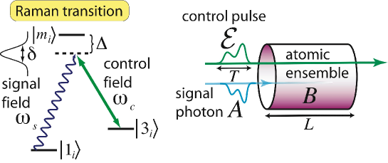
Figure 1: Left: the level structure of the atoms comprising a quantum memory for broadband photons, with bandwidth $\delta$. Right: a schematic of the readin process for the quantum memory.

The results in this paper are one dimensional, in the sense that they apply to an ensemble which is much longer, along the propagation direction, than it is wide (with a Fresnel number [15] of order unity or less). A fully three dimensional model, capable of investigating the memory evolution with non-colinear signal and control fields, as well as the limits imposed on memory fidelity by spontaneous emission and motional decoherence, is the subject of a parallel publication [16]. In the one-dimensional limit, we show that the full propagation problem is simplified greatly by the use of an appropriate modal decomposition.

In [8] it is shown that the Raman interaction of a CW driving field with an atomic vapour can be decomposed as a set of two-mode squeezing transformations between light and matter. These modes characterise both the temporal structure of the Stokes light produced, and the spatial structure of the correlated spin wave generated in the ensemble. Recent work [9] has verified the exact nature of this squeezed mode decomposition, shedding light on the properties of such multimode interactions. In particular the authors show how canonical evolution of the field operators fixes the relationship between the input and output modes for the problem. This analysis of Stokes generation is closely connected to the description of the quantum memory we present here. We show in this paper that the structure of the dynamical equations describing both systems guarantees canonical evolution of the optical and spin-wave field operators. Their commutation relations are automatically preserved by the solution and we do not need to impose this property as an extra condition. That is, the mode structure is intrinsic to the classical electrodynamics of the problem, rather than being intrinsically quantum mechanical. We also show that, if group velocity dispersion can be neglected, the evolution of the quantum memory subject to a control pulse of arbitrary shape is related to the simple case of a CW control field by a coordinate transformation. The evolution has a natural decomposition in terms of a set of mutually orthogonal input and output modes, and these modes are found to be related by a time-reversal-like symmetry. Each mode is associated with a singular value which quantifies the efficiency of the transfer from the input light-field mode to the stored spin-wave mode. The magnitudes of the singular values depend only upon a single parameter which represents the strength of the coupling of the quantum memory to the incident signal photon.

2 Model

The control pulse, together with the ensemble of three-level atoms, may be treated as a two-level system, whose absorptive properties are determined by the control field. In [7] a fully quantum mechanical treatment for the spontaneous initiation of Raman scattering in a one-dimensional atomic ensemble is introduced. The arguments may be adapted to describe the propagation of a signal photon through the memory cell.

The $i^{\mathrm{th}}$ atom in the ensemble with energy eigenstates $|j_{i}\rangle$, at position $z_{i}$ and time $t$, couples to the electromagnetic field via the dipole interaction Hamiltonian (setting $\hbar=1$):

$$\mathcal{H}^{i}_{\mathrm{int}}= -\sum_{j,k}\sigma^{i}_{jk}\mathsf{d}^{i}_{jk}.\mathsf{E}(t,z_{i}).$$ (1)

The transition projection operators are defined by

$$\sigma^{i}_{jk}(t=0)\equiv|j_{i}\rangle\langle k_{i}|,$$ (2)

in the Heisenberg picture. The electric field $\mathsf{E}(t,z)=\mathsf{E}_{s}(t,z)+\mathsf{E}_{c}(t,z)$ is made up of a classical control field with central frequency $\omega_{c}$ and polarisation unit vector $\epsilon_{c}$,

$$\mathsf{E}_{c}(t,z)=\epsilon_{c}E_{c}\mathcal{E}(t,z)\exp{[-\mathrm{i}\omega_{c}(t-z/c)]}+\mathrm{c.c.},$$ (3)

and a single photon signal field with polarisation unit vector $\epsilon_{s}$, written in quantized notation as

$$\mathsf{E}_{s}(t,z)=\epsilon_{s}\mathrm{i}\int_{0}^{\infty}g(\omega)a(t,\omega)\exp[{\mathrm{i}\omega z/c}]\,\rmd\omega+\mathrm{h.c.}.$$ (4)

The spatio-temporal dependence of the control field is contained in the dimensionless envelope function $\mathcal{E}(t,z)$, which is scaled so that its maximum value is $1$. $E_{c}$ is then the peak amplitude of the control field. In the Heisenberg picture, the mode annihilation operators satisfy the usual equal-time commutation relations

$$\left[a(t,\omega),a^{\dagger}(t,\omega^{\prime})\right]=\delta(\omega-\omega^{\prime}).$$ (5)

The mode amplitude is given by $g(\omega)\equiv\sqrt{\frac{\omega}{4\pi\epsilon_{0}\mathcal{A}c}}$, where $\mathcal{A}$ is the cross-sectional area of the region within the ensemble excited by the optical fields, $c$ is the speed of light and $\epsilon_{0}$ is the permittivity of free space [17]. We have also defined the transition dipole moments by

$$\mathsf{d}^{i}_{jk}\equiv\langle j_{i}|\mathsf{d}^{i}|k_{i}\rangle,$$ (6)

where $\mathsf{d}^{i}$ is the electric dipole moment operator for the $i^{\mathrm{th}}$ atom.

The signal pulse amplitude is represented by the ‘slowly varying’ operator

$$A(t,z)\equiv\exp{[\mathrm{i}\omega_{s}(t-z/v_{s})]}\frac{1}{\sqrt{2\pi}}\int_{-\infty}^{\infty}a(t,\omega)\exp{[\mathrm{i}\omega z/v_{s}]}\,\rmd\omega,$$ (7)

where $\omega_{s}$ is the centre frequency of the pulse, and $v_{s}$ is the group velocity of the signal field. The spin wave to which the signal excitation is transferred is represented by the corresponding operator [8]

$$B(t,z)\equiv\frac{1}{\delta z\sqrt{n\mathcal{A}}}\sum_{\beta}\sigma^{\beta}_{13}(t)\exp{\left\{-\mathrm{i}\left[(\omega_{s}-\omega_{c})t-\left(\frac{\omega_{s}}{v_{s}}-\frac{\omega_{c}}{v_{c}}\right)z_{\beta}\right]\right\}},$$ (8)

with $v_{c}$ the group velocity of the control field. Here the index $\beta$ runs over all the atoms lying within a thin slice of the ensemble of thickness $\delta z$, centred at position $z$. $n$ is the atomic number density. The operators $A$ and $B$ act as continuous-mode bosonic annihilation operators for the signal pulse and atomic ensemble respectively; they satisfy the canonical commutation relations

$$[A(t,0),A^{\dagger}(t^{\prime},0)]= \delta(t-t^{\prime}),$$ (9)

$$[B(0,z),B^{\dagger}(0,z^{\prime})]= \delta(z-z^{\prime}),$$ (10)

where the Dirac delta function $\delta(x)$ is the derivative of the Heaviside step function

$$\Theta(x)=\cases{1&for $x\geq 0$;\\ 0&for $x<0$.\\ }$$ (11)

3 Propagation

Provided that the common detuning $\Delta$ of the signal and control pulses from single photon resonance is much larger than the signal photon bandwidth $\delta$, the excited state $|m_{i}\rangle$ can be adiabatically eliminated. If the ensemble is prepared in the collective groundstate $|0\rangle\equiv\bigotimes_{i}|1_{i}\rangle$, and if the population of the metastable state $|3_{i}\rangle$ is assumed to remain negligible, a linear theory can be used. The Maxwell-Bloch equations, in the slowly varying envelope approximation, are then found to be:

$$\partial_{t}B(t,z)=-\gamma^{*}\mathcal{E}^{*}(t,z)A(t,z),$$ (12)

and

$$\left[\partial_{z}+\frac{1}{v_{s}}\partial_{t}\right]A(t,z)=\gamma\mathcal{E}(t,z)B(t,z).$$ (13)

The coupling constant $\gamma$ is given, to first order, by

$$\gamma=\sqrt{\frac{n\omega_{s}}{2\epsilon_{0}c}}\frac{d_{s}^{*}d_{c}E_{c}}{\Delta},$$ (14)

with $d_{s}$, $d_{c}$ the dominant transition dipole moments:

$$d_{s}\equiv\mathsf{d}^{i}_{m1}\cdot\mathsf{\epsilon}_{s}\;;\qquad d_{c}\equiv\mathsf{d}^{i}_{m3}\cdot\mathsf{\epsilon}_{c}\,,\qquad\forall i.$$ (15)

The dephasing of the material excitation $B$ can be modelled by appending a decay term and a Langevin operator [18] to (12), but here for simplicity we neglect the effects of decoherence: this remains a good approximation if the transverse coherence decay time of the spin wave is much larger than the duration of the signal pulse. We define the local time $\tau\equiv t-z/v_{s}$, whence we obtain

$$\partial_{\tau}B(\tau,z)= -\gamma^{*}\mathcal{E}^{*}(\tau-\kappa z)A(\tau,z);$$ (16)

$$\partial_{z}A(\tau,z)= \quad\gamma\mathcal{E}(\tau-\kappa z)B(\tau,z).$$ (17)

Here we have expressed the functional form of the control pulse in terms of the dispersivity $\kappa$, given by

$$\kappa\equiv\frac{1}{v_{c}}-\frac{1}{v_{s}}.$$ (18)

In the case that dispersion can be neglected, so that $v_{c}\approx v_{s}$, the control field becomes a function of $\tau$ only, and a Laplace transform over the spatial variable $z$ yields an analytic solution to the coupled equations (16,17) [7]. This is the situation with which the bulk of this paper is concerned. However, even if $v_{c}\neq v_{s}$, the solutions can be obtained numerically [9]. In the general case, for arbitrary $\kappa$, they have the following form:

$$A(\tau,L)= \int_{0}^{T}C_{A}(\tau,\tau^{\prime})A(\tau^{\prime},0)\,\rmd\tau^{\prime}+\int_{0}^{L}S_{A}(\tau,z^{\prime})B(0,z^{\prime})\,\rmd z^{\prime},$$ (19)

$$B(T,z)= \int_{0}^{L}C_{B}(z,z^{\prime})B(0,z^{\prime})\,\rmd z^{\prime}-\int_{0}^{T}S_{B}(z,\tau^{\prime})A(\tau^{\prime},0)\,\rmd\tau^{\prime},$$ (20)

where $L$ is the length of the ensemble, and $T$ is the duration of the readin process. The integral kernels $C_{A,B},S_{A,B}$ are Green’s functions which propagate the boundary conditions $A(\tau,0)$ and $B(0,z)$. Because we write the solutions at the output of the ensemble, after the pulses have fully traveled through it, these are input-output, or scattering, relations.

4 Unitarity and Mode Decomposition

4.1 Quantum memory dynamics

The coordinates $(\tau,z)$ may be discretized over an arbitrarily fine mesh, and then the above equations (19,20) are represented (as in [9]) to any chosen accuracy by the matrix equations

$$\mbox{\boldmath$A$}_{L}= \mbox{\boldmath$C$}_{A}\mbox{\boldmath$A$}_{0}+\mbox{\boldmath$S$}_{A}\mbox{\boldmath$B$}_{0};$$ (21)

$$\mbox{\boldmath$B$}_{T}= \mbox{\boldmath$C$}_{B}\mbox{\boldmath$B$}_{0}-\mbox{\boldmath$S$}_{B}\mbox{\boldmath$A$}_{0},$$ (22)

with column vectors $\mbox{\boldmath$A$}_{0}$,$\,\mbox{\boldmath$B$}_{0}$ replacing the initial signal and spin-wave amplitudes, and with $\mbox{\boldmath$A$}_{L}$,$\mbox{\boldmath$B$}_{T}$ replacing the final signal and spin-wave amplitudes. The integral kernels are replaced by the matrices $\mbox{\boldmath$C$}_{A,B}$ and $\mbox{\boldmath$S$}_{A,B}$. This transformation should be unitary, since it describes the evolution of quantum mechanical operators, but it is not immediately obvious how this is guaranteed by the equations (16,17). As with an ordinary lossless beamsplitter, it is conservation of flux which constrains the solution. To see this, consider the following continuity relation implied by the evolution equations:

$$\partial_{z}A^{\dagger}(\tau,z)A(\tau,z)+\partial_{\tau}B^{\dagger}(\tau,z)B(\tau,z)=0.$$ (23)

Integrating this expression over a rectangle in $(\tau,z)$-space yields the expression

$$\int_{0}^{\tau}A^{\dagger}(\tau^{\prime},z)A(\tau^{\prime},z)\,\rmd\tau^{\prime}+\int_{0}^{z}B^{\dagger}(\tau,z^{\prime})B(\tau,z^{\prime})\,\rmd z^{\prime}=F_{\tau}(\tau)+F_{z}(z),$$ (24)

where $F_{z}$ and $F_{\tau}$ are functions determined by the boundary conditions. Successively setting $(\tau,z)=(0,0),(0,L),(T,0),(T,L)$, we derive the flux-excitation conservation condition

$$\mbox{\boldmath$A$}_{L}^{\dagger}\cdot\mbox{\boldmath$A$}_{L}+\mbox{\boldmath$B$}_{T}^{\dagger}\cdot\mbox{\boldmath$B$}_{T}=\mbox{\boldmath$A$}_{0}^{\dagger}\cdot\mbox{\boldmath$A$}_{0}+\mbox{\boldmath$B$}_{0}^{\dagger}\cdot\mbox{\boldmath$B$}_{0},$$ (25)

which must hold for arbitrary initial amplitudes $\mbox{\boldmath$A$}_{0},\mbox{\boldmath$B$}_{0}$. Here the ‘dot’ denotes the scalar product of two vectors: $\mbox{\boldmath$A$}\cdot\mbox{\boldmath$B$}\equiv\mbox{\boldmath$A$}^{\mathsf{T}}\mbox{\boldmath$B$}$, where the superscript $\mathsf{T}$ indicates matrix transposition. The dagger denotes Hermitian conjugation of operators. When applied to an ordinary matrix, or a complex number, it is equivalent to complex conjugation. In order to avoid confusion, we do not use a dagger to indicate the composition of transposition with complex conjugation. We can cast the condition (25) in a more compact form:

$$\mbox{\boldmath$X$}^{\dagger}\cdot\mbox{\boldmath$X$}=\mbox{\boldmath$X$}_{0}^{\dagger}\cdot\mbox{\boldmath$X$}_{0},$$ (26)

where we have defined

$$\mbox{\boldmath$X$}\equiv\left(\begin{array}[]{c}\mbox{\boldmath$A$}_{L}\\ \mbox{\boldmath$B$}_{T}\end{array}\right)=\mbox{\boldmath$U$}\mbox{\boldmath$X$}_{0},$$ (27)

with

$$\mbox{\boldmath$X$}_{0}\equiv\left(\begin{array}[]{c}\mbox{\boldmath$A$}_{0}\\ \mbox{\boldmath$B$}_{0}\end{array}\right)\;;\quad\mbox{\boldmath$U$}\equiv\left(\begin{array}[]{cc}\mbox{\boldmath$C$}_{A}&\mbox{\boldmath$S$}_{A}\\ -\mbox{\boldmath$S$}_{B}&\mbox{\boldmath$C$}_{B}\end{array}\right)\;.$$ (28)

(26) then tells us that the transformation $\mbox{\boldmath$X$}_{0}\rightarrow\mbox{\boldmath$X$}$ preserves the norm of $\mbox{\boldmath$X$}_{0}$, and this fixes $U$ as unitary. The evolution of the operators describing the memory interaction is therefore canonical, as we would expect. This fact has important implications. In particular, multiplying out the relations $\mbox{\boldmath$U$}^{\mathsf{T}*}\mbox{\boldmath$U$}=\mbox{\boldmath$U$}\mbox{\boldmath$U$}^{\mathsf{T}*}=\mbox{\boldmath$I$}$ provides us with the conditions

$$\mbox{\boldmath$C$}_{A}^{\mathsf{T}*}\mbox{\boldmath$C$}_{A}+\mbox{\boldmath$S$}_{B}^{\mathsf{T}*}\mbox{\boldmath$S$}_{B}= \mbox{\boldmath$I$};$$ (29)

$$\mbox{\boldmath$C$}_{B}^{\mathsf{T}*}\mbox{\boldmath$C$}_{B}+\mbox{\boldmath$S$}_{A}^{\mathsf{T}*}\mbox{\boldmath$S$}_{A}= \mbox{\boldmath$I$},$$ (30)

along with a pair of antinormally ordered counterparts. We can now apply the Bloch-Messiah reduction [19] to (29). For (29), this consists in spectral decomposition [20] of the positive Hermitian matrix products $\mbox{\boldmath$C$}_{A}^{\mathsf{T}*}\mbox{\boldmath$C$}_{A}$ and $\mbox{\boldmath$S$}_{B}^{\mathsf{T}*}\mbox{\boldmath$S$}_{B}$. These must commute with one another, and therefore they are both rendered diagonal in the same orthonormal basis. Similar conclusions follow for the remaining equations ((30) and antinormal versions). As is shown in [9], the analysis reveals simple relationships between the singular value decompositions of the integral kernels, as follows:

$$C_{A}(\tau,\tau^{\prime})= \sum_{i=1}^{\infty}\phi_{i}(\tau)\mu_{i}\psi_{i}(\tau^{\prime}),$$ (31)

$$S_{B}(\tau^{\prime},z)= \sum_{i=1}^{\infty}\phi_{i}(z)\lambda_{i}\psi_{i}(\tau^{\prime}),$$ (32)

$$C_{B}(z,z^{\prime})= \sum_{i=1}^{\infty}\varphi_{i}(z)\mu_{i}\chi_{i}(z^{\prime}),$$ (33)

$$S_{A}(\tau,z^{\prime})= \sum_{i=1}^{\infty}\varphi_{i}(\tau)\lambda_{i}\chi_{i}(z^{\prime}),$$ (34)

where the functions $\{\phi_{i}\}$, $\{\psi_{i}\}$, $\{\varphi_{i}\}$, $\{\chi_{i}\}$, each form a complete orthonormal basis, and where $\lambda_{i}$,$\mu_{i}$ are real, positive singular values for which

$$\lambda_{i}^{2}+\mu_{i}^{2}=1\quad\forall i.$$ (35)

Equations (31-35), when substituted into (19,20), imply a set of independent beam-splitter transformations of ensemble modes and light-field modes.

4.2 Application to Stokes scattering

Finally, we note that the above arguments apply in slightly altered form to the analysis of stimulated Stokes scattering presented in [9]. In that case, Stokes photons and spin wave excitations are generated in pairs, and accordingly it is the flux difference that is conserved by the Maxwell-Bloch equations (where now the operator $A$ represents the amplitude of the Stokes field):

$$\partial_{\tau}B(\tau,z)= \gamma^{*}\mathcal{E}^{*}(\tau-\kappa z)A^{\dagger}(\tau,z);$$ (36)

$$\partial_{z}A(\tau,z)= \gamma\mathcal{E}(\tau-\kappa z)B^{\dagger}(\tau,z).$$ (37)

The resulting flux-excitation conditions are altered slightly, corresponding to swapping the plus sign appearing in (25) for a minus sign. We can write them in the form

$$\mbox{\boldmath$X$}^{\dagger\mathsf{T}}\mbox{\boldmath$Z$}\mbox{\boldmath$X$}=\mbox{\boldmath$X$}_{0}^{\dagger\mathsf{T}}\mbox{\boldmath$Z$}\mbox{\boldmath$X$}_{0};$$ (38)

$$\mbox{\boldmath$X$}^{\mathsf{T}}\mbox{\boldmath$Z$}\mbox{\boldmath$X$}^{\dagger}=\mbox{\boldmath$X$}_{0}^{\mathsf{T}}\mbox{\boldmath$Z$}\mbox{\boldmath$X$}_{0}^{\dagger},$$ (39)

where

$$\mbox{\boldmath$Z$}\equiv\left(\begin{array}[]{cc}\mbox{\boldmath$I$}&0\\ 0&-\mbox{\boldmath$I$}\end{array}\right)$$

is the $z$-projection Pauli spin matrix. The solution to (36,37) is now written

$$\mbox{\boldmath$X$}=\mbox{\boldmath$C$}\mbox{\boldmath$X$}_{0}+\mbox{\boldmath$S$}\mbox{\boldmath$X$}_{0}^{\dagger},$$ (40)

where the matrices $C$,$S$ are of the form

$$\mbox{\boldmath$C$}\equiv\left(\begin{array}[]{cc}\mbox{\boldmath$C$}_{A}&0\\ 0&\mbox{\boldmath$C$}_{B}\end{array}\right)\;;\quad\mbox{\boldmath$S$}\equiv\left(\begin{array}[]{cc}0&\mbox{\boldmath$S$}_{A}\\ -\mbox{\boldmath$S$}_{B}&0\end{array}\right).$$ (41)

Substitution of this ansatz into the sum of (38) and (39) provides us with the conditions

$$\mbox{\boldmath$C$}^{\mathsf{T}*}\mbox{\boldmath$Z$}\mbox{\boldmath$C$}+\mbox{\boldmath$S$}^{\mathsf{T}}\mbox{\boldmath$Z$}\mbox{\boldmath$S$}^{*}= \mbox{\boldmath$I$};$$ (42)

$$\mbox{\boldmath$C$}^{\mathsf{T}*}\mbox{\boldmath$Z$}\mbox{\boldmath$S$}+\mbox{\boldmath$S$}^{\mathsf{T}}\mbox{\boldmath$Z$}\mbox{\boldmath$C$}^{*}= 0.$$ (43)

These relations fix the inverse transformation to (40) as

$$\mbox{\boldmath$X$}_{0}=\mbox{\boldmath$Z$}\mbox{\boldmath$C$}^{\mathsf{T}*}\mbox{\boldmath$X$}-\mbox{\boldmath$Z$}\mbox{\boldmath$S$}^{\mathsf{T}}\mbox{\boldmath$X$}^{\dagger},$$ (44)

and substitution of this into the flux conditions (38,39) yields the antinormal condition

$$\mbox{\boldmath$C$}\mbox{\boldmath$C$}^{\mathsf{T}*}-\mbox{\boldmath$S$}\mbox{\boldmath$S$}^{\mathsf{T}*}=\mbox{\boldmath$Z$}.$$ (45)

Inspection of the components of the equations (42,45) reveals all the conditions required of the matrices $\mbox{\boldmath$C$}_{A,B},\mbox{\boldmath$S$}_{A,B}$ to apply the Bloch-Messiah reduction. This then yields a mode decomposition for the Stokes scattering problem, which is given explicitly in [9] and used to identify the dynamics with that of the well-known two-mode squeezer. The property of separability which allows the dynamics to be understood in terms of independent modes is therefore also related to a form of flux conservation.

We now show that when dispersion can be neglected, the relations (31–34), describing the memory, simplify even further. Under this approximation, only one set of functions $\{\phi_{i}\}$, which may be computed by numerical diagonalisation of a known function, is involved in the dynamics. This approximation is consistent with the requirement of adiabaticity $\delta\ll\Delta$ for a broadband signal photon, since the refractive index of the ensemble varies slowly with frequency far from resonance.

5 Dispersionless case

We return to the equations (16,17), and set $\kappa=0$, so that the $z$-dependence of the control field $\mathcal{E}$ vanishes. We introduce the dimensionless ‘control pulse area’

$$\epsilon=\epsilon(\tau)\equiv\gamma\sqrt{\frac{L}{E}}\int_{0}^{\tau}|\mathcal{E}(\tau^{\prime})|^{2}\,\rmd\tau^{\prime},$$ (46)

where the factor $E\equiv\int_{0}^{T}|\mathcal{E}(\tau^{\prime})|^{2}\,\rmd\tau^{\prime}$ appears in order to normalise this new variable so that it takes values between $0$ and $C\equiv\gamma\sqrt{LE}$. We also introduce a normalised spatial variable $\zeta\equiv\gamma z\sqrt{E/L}$. Again, $\zeta$ runs from $0$ to $C$. For simplicity we have set $\gamma$ to be real; alternatively any complex phase in $\gamma$ can always be incorporated into the field $\mathcal{E}$. In this new coordinate system the equations (16,17) become

$$\partial_{\zeta}\alpha=\beta\;;\;\;\;\partial_{\epsilon}\beta=-\alpha,$$ (47)

where we have defined the dimensionless annihilation operators $\alpha(\epsilon,\zeta)\equiv\sqrt{E}A(\tau,z)/\mathcal{E}(\tau)$, and $\beta(\epsilon,\zeta)\equiv\sqrt{L}B(\tau,z)$. We have now eliminated the variation of the control field from the dynamical equations; the problem is reduced to that of a CW control field coupled to the ensemble for a brief time. The solutions for the signal amplitude $\alpha_{C}(\epsilon)\equiv\alpha(\epsilon,C)$ at the exit face of the ensemble, and the spin wave amplitude $\beta_{C}(\zeta)\equiv\beta(C,\zeta)$ at the end of the readin process, are given in terms of the initial conditions $\alpha(\epsilon,\zeta=0)=\alpha_{0}(\epsilon)$ and $\beta(\epsilon=0,\zeta)=\beta_{0}(\zeta)$ by the expressions

$$\alpha_{C}(\epsilon)= \int_{0}^{C}\left[G_{1}(\epsilon-x,C)\alpha_{0}(x)+G_{0}(C-x,\epsilon)\beta_{0}(x)\right]\,\rmd x,$$ (48)

$$\beta_{C}(\zeta)= \int_{0}^{C}\left[G_{1}(\zeta-x,C)\beta_{0}(x)-G_{0}(C-x,\zeta)\alpha_{0}(x)\right]\,\rmd x.$$ (49)

There are now just two integral kernels, given by

$$G_{0}(p,q)\equiv J_{0}\left(2\sqrt{pq}\right),$$ (50)

$$G_{1}(p,q)\equiv \delta(p)-\Theta(p)\sqrt{\frac{q}{p}}J_{1}\left(2\sqrt{pq}\right),$$ (51)

with the $n^{\mathrm{th}}$ Bessel function of the first kind denoted by $J_{n}$, and where the Heaviside step function (11) ensures that the convolutions in (48,49) respect causality. We write the matrix representation of the solution (48,49) as

$$\mbox{\boldmath$\alpha$}_{C}= \mbox{\boldmath$G$}_{1}\mbox{\boldmath$\alpha$}_{0}+\mbox{\boldmath$G$}_{0}\mbox{\boldmath$\beta$}_{0}\,;$$ (52)

$$\mbox{\boldmath$\beta$}_{C}= \mbox{\boldmath$G$}_{1}\mbox{\boldmath$\beta$}_{0}-\mbox{\boldmath$G$}_{0}\mbox{\boldmath$\alpha$}_{0}.$$ (53)

Note that both of the matrices $\mbox{\boldmath$G$}_{1}$ and $\mbox{\boldmath$G$}_{0}$ are persymmetric. That is, they are both symmetric about their main anti-diagonal (or skew diagonal). To see this, observe that the integral kernel $G_{1}$ (as it appears in (48)) varies only as a function of the quantity $\epsilon-x$. That is to say, its contours are all parallel to the line $\epsilon=x$, which corresponds to the main diagonal of $\mbox{\boldmath$G$}_{1}$. $\mbox{\boldmath$G$}_{1}$ is therefore invariant under reflection about its main anti-diagonal. The corresponding symmetry for $\mbox{\boldmath$G$}_{0}$ follows from the Hermiticity of the kernel $G_{0}(p,q)$ in its arguments. These symmetries allow us to decompose the kernels using input and output modes related by time reversal (or equivalently space reversal):

$$G_{0}(C-x,\epsilon)= \sum_{i=1}^{\infty}\phi_{i}(\epsilon)\lambda_{i}\phi_{i}(C-x),$$ (54)

$$G_{1}(\epsilon-x,C)= \sum_{i=1}^{\infty}\phi_{i}(\epsilon)\mu_{i}\phi_{i}(C-x),$$ (55)

where there is now just a single set of real modefunctions $\{\phi_{i}\}$ such that

$$\int_{0}^{C}\phi_{i}(x)\phi_{j}(x)\,\rmd x=\delta_{ij}.$$ (56)

6 State transfer

Following the treatment in [8] we define output mode operators using the mode expansions

$$\alpha_{C}(\epsilon)\equiv \sum_{i}\phi_{i}(\epsilon)A_{i},$$ (57)

$$\beta_{C}(\zeta)\equiv \sum_{i}\phi_{i}(\zeta)B_{i}.$$ (58)

For the input operators, we use the time-reversed expansions

$$\alpha_{0}(\epsilon)\equiv \sum_{i}\phi_{i}(C-\epsilon)a_{i},$$ (59)

$$\beta_{0}(\zeta)\equiv \sum_{i}\phi_{i}(C-\zeta)b_{i}.$$ (60)

The solutions (48,49) can now be written in the form

$$A_{i}= \mu_{i}a_{i}+\lambda_{i}b_{i}\,,$$ (61)

$$B_{i}= \mu_{i}b_{i}-\lambda_{i}a_{i}\,,$$ (62)

with

$$[A_{i},A_{j}^{\dagger}]=[B_{i},B_{j}^{\dagger}]=[a_{i},a_{j}^{\dagger}]=[b_{i},b_{j}^{\dagger}]=\delta_{ij}.$$ (63)

Equations (61,62) show that the interaction of a signal photon with the memory cell can be viewed as a beamsplitter transformation on a mode-by-mode basis. Maximising the fidelity of the state transfer then amounts to minimising the terms $\mu_{i}a_{i}$. The magnitudes of the $\mu_{i}$ are determined by the coupling parameter $C$; a large value corresponds to an optically thick ensemble — a high absorption. In figure 2 the singular values of the matrix $\mbox{\boldmath$G$}_{0}$ are plotted as a function of $C$. These are found by multiplying (54) through by the $i^{\mathrm{th}}$ input mode and integrating, using (56). We obtain the following relation:

$$\int_{0}^{C}G_{0}(C-y,x)\phi_{i}(C-y)\,\rmd y=\lambda_{i}\phi_{i}(x),$$ (64)

corresponding to the simple eigenvalue equation

$$\int_{0}^{C}J_{0}(2\sqrt{xy})\phi_{i}(y)\,\rmd y=\lambda_{i}\phi_{i}(x),$$ (65)

which we solve numerically using a $500$ by $500$ square grid. We see that the interaction is dominated by the lowest mode for small $C$, but as $C$ increases, higher modes become significantly coupled. Modematching is therefore particularly important when the interaction is weak, as is the case for large detuning. Near-complete state transfer for the lowest mode ($\lambda_{1}\approx 1$) can be achieved for an ensemble with a coupling strength $C\geq 2$.

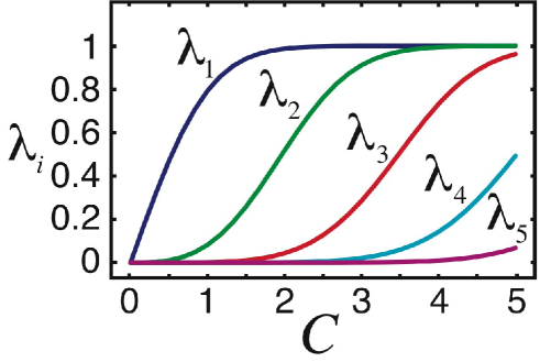
Figure 2: The five largest singular values of the kernel $\mbox{\boldmath$G$}_{0}$, plotted as a function of the coupling parameter $C$. The singular values are necessarily positive; for clarity they are plotted both above and below the origin.

7 Modematching

The efficiency of the memory is greatest for the lowest mode $\phi_{1}$. Therefore we require that the shape of this mode in real time matches the temporal structure of the signal photon wavepacket we send into our memory cell. The relationship between the shapes of the normalised real time input modes $\Phi_{i}(\tau)$, and the mode shapes as a function of control pulse area $\epsilon$, is determined by the temporal shape of the control field. The connection is straightforward,

$$\Phi_{i}(\tau)=\sqrt{\frac{C}{E}}\mathcal{E}(\tau)\phi_{i}[C-\epsilon(\tau)],$$ (66)

but not analytically invertible, so a simple optimisation was performed in order to find the control pulse shape which matches a given input photon to the memory mode. The result for a signal photon with a Gaussian input profile, matched to the mode $\phi_{1}(C-\epsilon)$ with the highest coupling, and the simplest shape, is shown in figure 3, for $C=2$. The photon is almost completely absorbed, although a small portion remains, due to the limitations of the modematching optimisation.

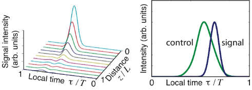
Figure 3: Top: the intensity $\langle A^{\dagger}(\tau,z)A(\tau,z)\rangle$ of a Gaussian signal photon as it propagates through an atomic ensemble with $C=2$. That is, a Fock state $|1_{\xi}\rangle\equiv a_{\xi}^{\dagger}|\mathrm{vac}\rangle$, where $a_{\xi}\equiv\int_{-\infty}^{\infty}\xi(\tau)A(\tau,0)\,\rmd\tau$ destroys a photon with a wave packet amplitude $\xi(\tau)\propto\exp{\{-2\ln 2[(\tau-\tau_{0})/\sigma]^{2}\}}$, with $\sigma=1/8$, $\tau_{0}=T/2$ and $T=L=1$. $|\mathrm{vac}\rangle$ denotes the vacuum. The absorption is nearly complete; it is limited by the quality of the modematching optimisation. Bottom: the optimised control field intensity (blue/black) is shown alongside the initial signal field intensity (green/grey). The latter has been scaled for clarity. The lowest mode (corresponding to the largest singular value $\lambda_{1}$) was used in the optimisation.

8 Readout

Once a properly modematched photon has been read in to the quantum memory, the ensemble is left in the output mode $\phi_{1}(\zeta)$, with probability amplitude $\lambda_{1}$. We now consider the effect of sending a second control pulse, propagating in the same direction as the initial control pulse, into the ensemble. The centre frequency, bandwidth and intensity of this readout pulse may differ from that of the first control pulse (herein the readin pulse). We can use all of the results developed thus far to analyse the interaction of the readout pulse with the ensemble, but we should be careful to keep track of any parameters which differ between the readin and readout stages. Let us use a superscript $r$ to indicate those quantities associated with the readout. If there is no significant change in the control and signal group velocities at readout (so that $v_{c}^{r}\approx v_{s}^{r}\approx v_{c}\approx v_{s}$), then the readout spin wave annihilation operator $B^{r}$ is phasematched to the readin spin wave operator $B$. That is, since the Stokes shift $\omega_{s}-\omega_{c}=\omega_{s}^{r}-\omega_{c}^{r}$ is fixed, the phase factor appearing in (8) is unchanged at readout, and we have $B^{r}(0,z)=B(T,z)$. Here again we have neglected any decoherence of the spin wave over the storage period. This provides us with one boundary condition; the second is that the signal field begins in its vacuum state at the start of the readout process:

$$\langle A^{r\dagger}(\tau,0)A^{r}(\tau,0)\rangle=0\,,\qquad\forall\tau.$$ (67)

At the end of the readout process, some portion of the stored excitation has been transferred back to the optical field. The efficiency of the readout depends upon the degree to which the spin wave mode $\phi_{1}(Cz/L)$ (written in terms of the ordinary spatial variable $z$) overlaps with the input modes for the readout process, which are of the form $\phi^{r}_{i}\left[C^{r}(1-z/L)\right]$. The functions $\{\phi_{i}^{r}\}$ solve the readout eigenvalue equation

$$\int_{0}^{C^{r}}J_{0}(2\sqrt{xy})\phi^{r}_{i}(y)\,\rmd y=\lambda^{r}_{i}\phi^{r}_{i}(x).$$ (68)

Each readout input mode $\phi^{r}_{i}\left[C^{r}(1-z/L)\right]$ is transferred to the optical field with amplitude $\lambda^{r}_{i}$, according to the relation (61), with these amplitudes set by the size of the readout coupling parameter $C^{r}$. A measure of the fidelity of the memory is the expectation value of the output photon number operator $\mathcal{N}$, which is just the probability of retrieving a photon from the ensemble at readout, given that a single modematched photon was sent in with the readin pulse. This retrieval probability is given by

$$\mathcal{N}\equiv \int_{0}^{T^{r}}\langle A^{r\dagger}(\tau,L)A^{r}(\tau,L)\rangle\,\rmd\tau$$

$$= \frac{1}{C^{r}}\int_{0}^{C^{r}}\langle\alpha^{r\dagger}(\epsilon^{r},C^{r})\alpha^{r}(\epsilon^{r},C^{r})\rangle\,\rmd\epsilon^{r}$$

$$= \frac{1}{C^{r}}\sum_{i=1}^{\infty}\langle A_{i}^{r\dagger}A_{i}^{\dagger}\rangle$$

$$= \frac{1}{C^{r}}\sum_{i=1}^{\infty}\lambda_{i}^{r2}\langle b_{i}^{r\dagger}b_{i}^{r}\rangle$$

$$= \lambda_{1}^{2}\sum_{i=1}^{\infty}\lambda_{i}^{r2}f_{i}^{2},$$ (69)

where in the penultimate step we have used the transformation (61) and the boundary condition (67) (setting $\langle a_{i}^{r\dagger}a_{i}^{r}\rangle=\langle b_{i}^{r\dagger}a_{i}^{r}\rangle=0$), and where we have defined the $i^{\mathrm{th}}$ overlap

$$f_{i}\equiv\frac{\sqrt{C^{r}C}}{L}\int_{0}^{L}\phi_{i}^{r}\left[C^{r}(1-z/L)\right]\phi_{1}(Cz/L)\,\rmd z.$$ (70)

In figure 4 the variation of $\mathcal{N}$ is plotted as a function of the readin and readout coupling parameters $C$ and $C^{r}$.

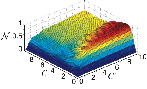
Figure 4: The photon retrieval probability $\mathcal{N}$ as a function of the readin and readout coupling parameters $C$ and $C^{r}$.

We observe that the retrieval probability is low if either $C$ or $C^{r}$ is small, as we expect from a weakly driven interaction. However, even if the photon is almost completely absorbed at readin, as is the case for the region $C\geq 2$, the probability of recovering the stored photon approaches unity only slowly as $C^{r}$ is increased. Furthermore, as the readin process is driven harder (as $C$ rises above $2$), the retrieval probability falls. These observations are explained by considering the overlaps $f_{i}$ of the readout modes with the spin wave mode. For small $C$, $\phi_{1}(Cz/L)$ is monotonic, and relatively flat. It therefore has a large overlap $f_{1}$ with the lowest readout mode, which for moderate values of $C^{r}$ is essentially the mirror image of the spin wave mode. As $C$ increases, the spin wave mode becomes more asymmetric, so that its overlap with the lowest readout mode falls. It is then necessary to pump the readout process harder, so that higher readout modes, with which the spin wave overlaps significantly, are efficiently coupled to the optical field. The readout efficiency therefore grows as the readin coupling $C$ is decreased. But as $C$ becomes small, so also does the probability that the photon was stored during the readin process at all. The retrieval probability is maximised along the line $C\approx 2$, which represents the optimal coupling for the readin process. However, a readout coupling parameter in excess of $10$ is required to achieve $\mathcal{N}\geq 0.95$.

The time reversal symmetry between the input and output modes makes the readout for this scheme a non-trivial problem. Simply repeating the readin process (so that $C=C^{r}$) results in poor performance of the memory. However, the dramatic increase in coupling strength required to extract the stored excitation fully, may make a naïve increase in control pulse energy at readout prohibitively difficult to realise. An alternative method to boost the coupling is by significantly reducing the bandwidth of the readout pulse, along with its detuning $\Delta^{r}$. The photon recovered from the memory in this way would be frequency-shifted (according to the Raman resonance condition), and temporally stretched (since its bandwidth would be greatly diminished as well). The temporal profile of the emitted photon would then be determined by the shape of the readout pulse, as well as the shapes of the output modes involved in the readout process. A ‘photon transducer’ with the ability to store broadband photons and convert them into narrowband photons with controllable frequency and shape could prove to be a useful tool for optical quantum information processing.

Finally, we comment that the symmetry of the modes suggests the possibility of reading the stored excitation using a readout pulse propagating in the reverse direction. Switching the propagation direction of the readout pulse would send $\phi_{i}(Cz/L)\rightarrow\phi_{i}\left[C(1-z/L)\right]$, so that the spin wave mode would overlap exactly with the lowest readout mode with $C=C^{r}$. Unfortunately, a counter propagating readout pulse would not have sufficient momentum to convert the spin wave into a counter propagating anti-Stokes photon. Another way to say this is that the readin and readout spin wave operators are not phasematched in this situation; the operator $B^{r}$ acquires a rapidly spatially varying phase factor, so that the overlap integrals $f_{i}$ vanish. However, an implementation of this scheme in the solid state (for example, replacing the atomic ensemble with an ensemble of semiconductor charge quantum dots [21]), might allow for the possibility of controlling the ensemble level structure with external fields. Then this kind of reverse readout might be achieved with the use of quasi-phasematching [22], in which the sign of the readout coupling parameter $C^{r}$ is periodically flipped along the length of the ensemble. If the wavevector of this modulation matches the size of the wavevector mismatch between the readin and readout spin waves, the readout photon can be retrieved. Alternatively, an adiabatic reversal of the sign of the Stokes shift over the whole ensemble, between the readin and readout stages (so that the energies of the states $|3_{i}\rangle$ and $|1_{i}\rangle$ are swapped at readout), would enable the phasematching of a high frequency counter propagating readout pulse, with the spin wave transferred to a counter propagating photon with lower frequency. Exploration of the possibilities for coherent manipulation of collective quanta in gaseous and solid-state ensembles will form the basis of continuing research.

9 Transverse profile

Here we briefly show that the modes $\{\phi_{i}\}$ also describe the transverse profile of the signal field. If the operators $\alpha$ and $\beta$ are allowed to depend upon the radial displacement $r$ from the $z$-axis, the Maxwell-Bloch equations, in the paraxial approximation [23], take the modified form

$$\left[\frac{1}{4C}\nabla_{\rho}^{2}+\mathrm{i}\partial_{\zeta}\right]\alpha(\mbox{\boldmath$\rho$},\zeta,\epsilon) =\mathrm{i}\beta(\mbox{\boldmath$\rho$},\zeta,\epsilon)\,;$$ (71)

$$\partial_{\epsilon}\beta(\mbox{\boldmath$\rho$},\zeta,\epsilon) =-\alpha(\mbox{\boldmath$\rho$},\zeta,\epsilon),$$ (72)

where $\rho$ is a normalised position vector for a point in the plane orthogonal to the propagation direction, a radial distance $r=\sqrt{2Lv_{s}/\omega_{s}}\rho$ from the $z$-axis. The extra term $\nabla_{\rho}^{2}$ is a $2$-dimensional Laplacian in the dimensionless cylindrical polar coordinates parameterising the point $\rho$. Here we have retained the assumption that the control field $\mathcal{E}$ has no radial dependence over the area $\mathcal{A}$. The dimensionless radial variable $\rho$ takes values from $0$ to $\rho_{\mathrm{max}}\equiv\sqrt{\omega_{s}/(2Lv_{s})}r_{\mathrm{max}}$, where $\pi r_{\mathrm{max}}^{2}\equiv\mathcal{A}$. The Fresnel number $\mathcal{F}$ is given by [15]

$$\mathcal{F} \equiv\left(\frac{\omega_{s}}{2\pi v_{s}}\right)\frac{\mathcal{A}}{L}$$ (73)

$$=\rho_{max}^{2}.$$

The limit of the paraxial approximation is usually defined by $\mathcal{F}=1$, so we set $\rho_{\mathrm{max}}=1$.

The solution to the equations (71,72) is found by alternately Fourier transforming the variables $(\mbox{\boldmath$\rho$},\zeta)$ and $(\mbox{\boldmath$\rho$},\epsilon)$ [23] [23]. We find:

$$\alpha_{C}(\mbox{\boldmath$\rho$},\epsilon) =\int_{\mathcal{A}}\,\rmd^{2}\mbox{\boldmath$\rho$}^{\prime}\int_{0}^{C}\,\rmd x[R(\mbox{\boldmath$\rho$}-\mbox{\boldmath$\rho$}^{\prime},C)G_{1}(\epsilon-x,C)\alpha_{0}(\mbox{\boldmath$\rho$}^{\prime},x)+$$ (74)

$$R(\mbox{\boldmath$\rho$}-\mbox{\boldmath$\rho$}^{\prime},C-x)G_{0}(C-x,\epsilon)\beta_{0}(\mbox{\boldmath$\rho$}^{\prime},x)]\,;$$

$$\beta_{C}(\mbox{\boldmath$\rho$},\zeta) =\int_{\mathcal{A}}\,\rmd^{2}\mbox{\boldmath$\rho$}^{\prime}\int_{0}^{C}\,\rmd x[R(\mbox{\boldmath$\rho$}-\mbox{\boldmath$\rho$}^{\prime},\zeta-x)G_{1}(\zeta-x,C)\beta_{0}(\mbox{\boldmath$\rho$}^{\prime},x)-$$ (75)

$$R(\mbox{\boldmath$\rho$}-\mbox{\boldmath$\rho$}^{\prime},\zeta)G_{0}(C-x,\zeta)\alpha_{0}(\mbox{\boldmath$\rho$}^{\prime},x)]\,,$$

where $\int_{\mathcal{A}}\,\rmd^{2}\mbox{\boldmath$\rho$}^{\prime}$ denotes an integral over a circular patch with unit radius, and where the diffraction kernel is given, up to a normalisation constant $N$, by

$$R(\mbox{\boldmath$\rho$},x)\equiv N\exp{\left(-\mathrm{i}C|\mbox{\boldmath$\rho$}|^{2}/x\right)}/x.$$ (76)

This kernel is singular for vanishing $x$, since the paraxial approximation breaks down in the near-field. However, in the limit that the interaction is negligible close to the exit face of the ensemble, we can make the replacement $R(\mbox{\boldmath$\rho$},x)\rightarrow R(\mbox{\boldmath$\rho$},C)$. The diffraction kernel then factorises out of the $\epsilon$ and $\zeta$ integrals in (74,75). We introduce the spectral decomposition

$$R(\mbox{\boldmath$\rho$}-\mbox{\boldmath$\rho$}^{\prime},C)=\sum_{j=0}^{\infty}\varphi_{j}(\mbox{\boldmath$\rho$})\sigma_{j}\varphi_{j}(\mbox{\boldmath$\rho$}^{\prime}),$$ (77)

where the $\sigma_{j}$ are real eigenvalues and $\{\varphi_{j}\}$ is a complete orthonormal set of paraxial modes, satisfying

$$\int_{\mathcal{A}}\varphi_{j}(\mbox{\boldmath$\rho$})\varphi^{*}_{k}(\mbox{\boldmath$\rho$})\,\rmd^{2}\mbox{\boldmath$\rho$}=\delta_{jk}.$$ (78)

We assume that the spatial profile of the signal field depends only upon the radial coordinate $\rho$. Cylindrical symmetry of the boundary conditions then allows us to neglect modes with any dependence on azimuthal angle. These cylindrically symmetric modes are then given by

$$\varphi_{j}(\rho)=e^{\mathrm{i}\rho^{2}}\phi_{j}^{1}(\rho^{2}),$$ (79)

where the superscript $1$ indicates that the function $\phi_{j}^{1}$ solves the eigenvalue equation (65) with $C$ set equal to $1$. We define input and output mode operators, as in (57,58,59,60), by the relations:

$$\alpha_{0}(\mbox{\boldmath$\rho$},\epsilon)\equiv\sum_{(i,j)=0}^{\infty}\phi_{i}(C-\epsilon)\varphi_{j}(\rho)a_{ij}\,;$$ (80)

$$\beta_{0}(\mbox{\boldmath$\rho$},\zeta)\equiv\sum_{(i,j)=0}^{\infty}\phi_{i}(C-\zeta)\varphi_{j}(\rho)b_{ij}\,,$$ (81)

and

$$\alpha_{C}(\mbox{\boldmath$\rho$},\epsilon)\equiv\sum_{(i,j)=0}^{\infty}\phi_{i}(\epsilon)\varphi_{j}(\rho)A_{ij}\,;$$ (82)

$$\beta_{C}(\mbox{\boldmath$\rho$},\zeta)\equiv\sum_{(i,j)=0}^{\infty}\phi_{i}(\zeta)\varphi_{j}(\rho)B_{ij}\,,$$ (83)

with

$$[A_{ij},A_{kl}^{\dagger}]=[B_{ij},B_{kl}^{\dagger}]=[a_{ij},a_{kl}^{\dagger}]=[b_{ij},b_{kl}^{\dagger}]=\delta_{ik}\delta_{jl}.$$ (84)

We then obtain the beamsplitter transformations:

$$A_{ij}=\sigma_{j}\left(\mu_{i}a_{ij}+\lambda_{i}b_{ij}\right)\,;$$ (85)

$$B_{ij}=\sigma_{j}\left(\mu_{i}b_{ij}-\lambda_{i}a_{ij}\right)\,.$$ (86)

The lowest mode is dominantly coupled, with $\sigma_{1}=0.995$. The shape of this dominant spatial mode is well approximated by a Gaussian with beam waist $w_{s}=1.45$ (in the normalised units of the variable $\rho$). The control should be slightly less tightly focussed, with a waist $w_{c}\geq 3w_{s}$, to justify the approximation that the control field may be treated as a train of plane waves. If such appropriately focussed Gaussian beams are used for the signal and control fields, only the lowest paraxial mode is involved in the interaction. The index $j$ may be dropped from the relations (85,86), and setting $\sigma_{1}\approx 1$, we recover the transformations (61,62), and the one-dimensional treatment is justified.

10 Experiment

We are currently developing an implementation of this scheme in atomic thallium vapour. The gross structure of thallium has a $\Lambda$-type triplet, where the excited $7s^{2}S_{1/2}$ state is coupled strongly to the ground state $6p^{2}P_{1/2}$ and the metastable state $6p^{2}P_{3/2}$ (with an electric-dipole-forbidden radiative lifetime of $0.16$ s). The splitting of these last two levels is very large (around $8000$ $\mathrm{cm}^{-1}$), so that the signal and control pulses remain spectrally distinct, even when their bandwidths are large. The more stringent limit on the bandwidth of the photon that can be stored comes from the adiabaticity condition: in order that no real population is transferred to the excited state, atomic collisions must occur at a negligible rate [24], and the signal bandwidth $\delta$ should be much smaller than the detuning $\Delta$. The interaction cross-section scales as the inverse square of this detuning, so a compromise must be made between the bandwidth $\delta$ that is stored and the length $L$ of the ensemble. We hope to demonstrate the storage and retrieval of ultraviolet pulses ($\sim 390$ nm) with $\delta\approx 10$ nm and pulse lengths of around $100$ fs.

11 Summary

We have shown that it is possible to map a broadband photon wavepacket into an atomic spin wave using a Raman interaction. The relationship between the input state, the storage state and the output is clarified by the introduction of a mode decomposition. The modes are expressed in terms of a single universal set of eigenfunctions of a particular integral kernel. The form of these eigenfunctions depends only on the coupling strength of the memory interaction, and not upon the shapes of the pulses.

References

- [1] J. I. Cirac, A. K. Ekert, S. F. Huelga, and C. Macchiavello. Distributed quantum computation over noisy channels. quant-ph/9803017, 1999.
- [2] Nicolas Gisin, Grigoire Ribordy, Wolfgang Tittel, and Hugo Zbinden. Quantum cryptography. quant-ph/0101098, 2001.
- [3] H.-J. Briegel, W. Dür, J. I. Cirac, and P. Zoller. Quantum repeaters: The role of imperfect local operations in quantum communication. Phys. Rev. Lett., 81:5932–5935, 1998.
- [4] Grover L. K. From schrodinger’s equation to quantum search algorithm. American Journal of Physics, 69(7):769–777, 2001.
- [5] Peter Shor. Polynomial-time algorithms for prime factorization and discrete logarithms on a quantum computer. SIAM J. Sci. Statist. Comput., 26:1484, 1997.
- [6] A. E. Kozhekin, K. Mølmer, and E. Polzik. Quantum memory for light. Phys. Rev. A, 62:033809, 2000.
- [7] M. G. Raymer and J. Mostowski. Stimulated Raman scattering: Unified treatment of spontaneous initiation and spatial propagation. Phys. Rev. A, 24(4):1980–1993, 1981.
- [8] M. G. Raymer. Quantum state entanglement and readout of collective atomic-ensemble modes and optical wave packets by stimulated Raman scattering. J. Mod. Opt., 51(12):1739–1759, 2004.
- [9] Wojciech Wasilewski and M.G. Raymer. Pairwise entanglement and readout of atomic-ensemble and optical wave-packet modes in traveling-wave Raman interactions. quant-ph/0512157. Submitted to Phys. Rev. A, 2005.
- [10] L-M. Duan, M. D. Lukin, J. I. Cirac, and P. Zoller. Long-distance quantum communication with atomic ensembles and linear optics. Nature, 414:413–418, 2001.
- [11] L-M. Duan, J. I. Cirac, and P. Zoller. Three-dimensional theory for interaction between atomic ensembles and free-space light. Phys. Rev. A, 66:023818, 2002.
- [12] M. Fleischhauer and M. D. Lukin. Quantum memory for photons: Dark-state polaritons. Am. Phys. Soc., 65:022814, 2002.
- [13] M. Fleischhauer, A. Immamoglu, and J. Marangos. Electromagnetically induced transparency: Optics in coherent media. Rev. Mod. Phys., 77:633, 2005.
- [14] Alexey V. Gorshkov, Axel André, Michael Fleischhauer, Anders S Sørensen, and Mikhail D. Lukin. Optimal storage of photon states in optically dense atomic media. quant-ph/0604037, 2006.
- [15] M. G. Raymer and I. A. Walmsley. Progress in Optics. Elsevier Science Publishers B.V., xxviii edition, 1990.
- [16] K. Surmacz et al. Storing broadband photons in an atomic quantum memory. Unpublished, 2006.
- [17] Rodney Loudon. The Quantum Theory of Light. Oxford University Press, 2004.
- [18] H. Haken. Cooperative phenomena. Rev. Mod. Phys., 47(1):97–121, 1975.
- [19] Samuel L. Braunstein. Squeezing as an irreducible resource. quant-ph/9904002, 1999.
- [20] M. A. Nielsen and I. L. Chuang. Quantum Computation and Quantum Information. Cambridge University Press, 2004.
- [21] Wang Yao, Ren-Bao Liu, and L. J. Sham. Theory of control of the spin-photon interface for quantum networks. Phys. Rev. Lett., 95:030504, 2005.
- [22] Robert W. Boyd. Nonlinear Optics. Academic Press, 1992.
- [23] M. G. Raymer and I. A. Walmsley. Quantum theory of spatial and temporal coherence properties of stimulated Raman scattering. Phys. Rev. A, 32(1):332–344, 1985.
- [24] M. G. Raymer and J. L. Carlsten. Simultaneous observations of stimulated Raman scattering and stimulated collision-induced fluorescence. Phys. Rev. Lett., 39:1326, 1977.