Scaling behavior of the adiabatic Dicke Model

Abstract

We analyze the quantum phase transition for a set of $N$-two level systems interacting with a bosonic mode in the adiabatic regime. Through the Born-Oppenheimer approximation, we obtain the finite-size scaling expansion for many physical observables and, in particular, for the entanglement content of the system.

Introduction.

Many-body systems have become of central interest in the realm of quantum information theory as training grounds to study static, dynamical and sharing properties of quantum correlations. It has been natural, then, to employ the entanglement as a tool to analyze quantum phase transitions, one of the most striking consequences of quantum correlations in many body systems nature ; osborne ; vida2 . In this letter, we study the Dicke super-radiant phase transition and obtain the finite size scaling behavior of the quantum correlations at criticality.

The Dicke model (DM) describes the interaction of $N$ two-level systems (qubits) with a single bosonic mode dicke , and has become a paradigmatic example of collective quantum behavior. It exhibits a second-order phase transition hepp , which has been studied extensively WH ; gilmore ; liberti . The continued interest in the DM arises from its broad application range phyrep and from its rich dynamics, displaying many non-classical features milburn ; brandes ; Hou ; orszagent . The ground state entanglement of the DM has been recently analyzed lambert ; lambert2 ; reslen , and some aspect of its finite size behavior has been obtained numerically. Finally, Vidal and Dusuel, vidal , obtained the critical exponents by a modified Holstein-Primakoff approach.

The exact treatment of the finite-size corrections to the Dicke transition is quite complicated and the study of some limiting cases can be useful. In this Letter we analyze the case of $N$ qubits coupled to a slow oscillator. We discuss on equal footings both the finite size and the thermodynamic limit of the model, thus allowing to obtain the phase transition as well as its precursors at finite $N$. Indeed, we obtain the dominant scaling behavior for some entanglement measures and the entire $1/N$ expansion for all of the relevant physical observables, such as the order parameter. Concerning the quantum correlations, we argue that what is really relevant for the critical behavior is the bi-partite entanglement between the oscillator mode and the set of two level systems.

Adiabatic limit.

The interaction of $N$ identical qubits with a bosonic mode is described by the Hamiltonian

$$H=\omega a^{\dagger}a+\Delta S_{x}+{\lambda}(a^{\dagger}+a)S_{z}/{\sqrt{N}}$$ (1)

where $\omega$ is the frequency of the oscillator, $\Delta$ is the transition frequency of the qubit and $\lambda$ is the coupling strength. The $S$’s are the total spin observables, ${S}_{\nu}=\sum_{i=1}^{N}{\sigma}_{\nu}^{i}$, where ${\sigma}_{\nu}^{i}$ is the $\nu$-th the Pauli matrix for the $i$-th qubit. $H$ is equivalent to the Dicke Hamiltonian dicke , obtained after the rotation $e^{i\pi S_{y}/4}$.

We assume a slow oscillator and work in the regime $\Delta\gg\omega$ by employing the Born-Oppenheimer approximation. As detailed in adiabatic , the procedure can be followed more plainly by rewriting the Hamiltonian of Eq. (1) as

$$H=\frac{\omega}{2}\left[P^{2}+Q^{2}+DS_{x}+\frac{LQ}{\sqrt{N}}S_{z}\right]\,,$$ (2)

where we have introduced the dimensionless parameters $D=2\Delta/\omega$, and $L=2\sqrt{2}\lambda/\omega$, together with the oscillator coordinates $Q=(a^{\dagger}+a)/\sqrt{2}$, and $P=i(a^{\dagger}-a)/\sqrt{2}$.

The basic assumption of the well-known adiabatic approximation is that the state of a composite system with one fast and one slowly changing part can be written as:

$$|\psi_{tot}\rangle=\int dQ\,\phi(Q)|Q\rangle\otimes|\chi(Q)\rangle$$ (3)

$|\chi(Q)\rangle$ is the eigenstate of the “adiabatic” qubit equation for each fixed value of the slow variable $Q$,

$$\left(DS_{x}+\frac{LQ}{\sqrt{N}}S_{z}\right)|\chi(Q)\rangle=E(Q)|\chi(Q)\rangle\,,$$ (4)

and can be written as the direct product of the eigenstates of each single qubit

$$|\chi(Q)\rangle=|\chi(Q)\rangle_{1}\otimes|\chi(Q)\rangle_{2}\otimes\dots\otimes|\chi(Q)\rangle_{N}\,.$$ (5)

As the qubits are identical, the lowest eigenstate of Eq. (4) has the form

$$|\chi_{0}(Q)\rangle=\left\{\frac{1}{\sqrt{2}}\left[A_{-}(Q)|+\rangle-A_{+}(Q)|-\rangle\right]\right\}^{\otimes N},$$ (6)

where $|\pm\rangle$ are the $\pm 1$ eigenstates of $\sigma_{z}$, and

$$A_{\pm}(Q)=\sqrt{{1\pm\frac{LQ}{\sqrt{N}\Theta(Q)}}}\,.$$ (7)

The eigenvalue corresponding to this state is given by

$$E_{0}(Q)=-N\Theta(Q)=-N\sqrt{D^{2}+\frac{L^{2}Q^{2}}{N}}\,.$$ (8)

This energy eigenvalue contributes an effective adiabatic potential felt by the slow bosonic mode. The total potential for the variable $Q$ is, therefore

$$U_{0}(Q)=\frac{\omega}{2}\left[Q^{2}-N\Theta(Q)\right]\,.$$ (9)

Introducing the dimensionless parameter $\alpha={L^{2}}/{2D}$, one can show that for $\alpha\leq 1$, the potential $U_{0}(Q)$ can be viewed as a broadened harmonic potential well with its minimum at $Q=0$. For $\alpha>1$, on the other hand, the coupling with the qubit produces a symmetric double well with minima at $Q=\pm Q_{0}=\pm{\sqrt{N}D}\sqrt{\alpha^{2}-1}/L$.

Ground state properties.

In order to obtain the fundamental level of the coupled system, the last step in the adiabatic procedure is the evaluation of the ground state wave function for the oscillator, $\phi_{0}(Q)$, to be inserted in Eq. (3). This wave function satisfies the one-dimensional time independent Schrödinger equation

$$\left(-\frac{\omega}{2}\frac{d^{2}}{dQ^{2}}+U_{0}(Q)\right)\phi_{0}(Q)=\varepsilon_{0}\phi_{0}(Q)\,,$$ (10)

where $\varepsilon_{0}$ is the lowest eigenvalue.

The ground-state properties can be easily studied in the adiabatic limit. It turns out that all of the expectation values can be expressed in terms of the quantity:

$$\Phi_{\nu}=\int_{-\infty}^{\infty}\phi_{0}^{2}(Q)\left({1+\frac{2\alpha}{ND}Q^{2}}\right)^{\nu}dQ\,,$$ (11)

which is shown below to depend only on $\alpha$ and $ND$.

For the average values of the various components of the total spin, one gets

$$\frac{\langle S_{x}\rangle}{N}=-\Phi_{-\frac{1}{2}}\,,\quad{\langle S_{y}\rangle}={\langle S_{z}\rangle}=0\,,$$ (12)

$$\frac{\langle S_{x}^{2}\rangle}{N^{2}}=\frac{1}{N}+\left(1-\frac{1}{N}\right)\Phi_{-1}\,,$$ (13)

$$\frac{\langle S_{z}^{2}\rangle}{N^{2}}=\left(1+\frac{1}{N}\right)-\frac{\langle S_{x}^{2}\rangle}{N^{2}}\,,\quad\frac{\langle S_{y}^{2}\rangle}{N^{2}}=\frac{1}{N}\,.$$ (14)

Furthermore, the order parameter can be obtained from

$$\frac{\langle H\rangle}{N}=\frac{\omega}{2}\left(\frac{\langle{P^{2}+Q^{2}}\rangle}{N}-D\Phi_{\frac{1}{2}}(N)\right)\,.$$ (15)

In the thermodynamic limit ($N\rightarrow\infty$) one gets the well-known second-order quantum phase transition at $\alpha=\alpha_{c}=1$, for which:

$$\frac{\langle S_{x}\rangle}{N}=\left\{\begin{array}[]{ll}-1&\hbox{$(\alpha\leq 1)$}\\ \hbox{$-\frac{1}{\alpha}$}&\hbox{$(\alpha>1),$}\\ \end{array}\right.$$ (16)

$$\frac{\langle S_{x}^{2}\rangle}{N^{2}}=\left\{\begin{array}[]{ll}1&\hbox{$(\alpha\leq 1)$}\\ \hbox{$\frac{1}{\alpha^{2}}$}&\hbox{$(\alpha>1),$}\\ \end{array}\right.\,\frac{\langle S_{z}^{2}\rangle}{N^{2}}=1-\frac{\langle S_{x}^{2}\rangle}{N^{2}}\,,\quad\frac{\langle S_{y}^{2}\rangle}{N^{2}}=0\,,$$ (17)

$$\frac{\langle{Q^{2}+P^{2}}\rangle}{N}=\left\{\begin{array}[]{ll}0&\hbox{$(\alpha\leq 1)$}\\ \hbox{$\frac{D^{2}}{L^{2}}\left(\alpha^{2}-1\right)$}&\hbox{$(\alpha>1),$}\\ \end{array}\right.$$ (18)

and, finally

$$\frac{E_{0}}{N}=\left\{\begin{array}[]{ll}-D&\hbox{$(\alpha\leq 1)$}\\ \hbox{$-\frac{D}{2}\left(\alpha+\frac{1}{\alpha}\right)$}&\hbox{$(\alpha>1),$}\\ \end{array}\right.$$ (19)

where $E_{0}=2\varepsilon_{0}/\omega$.

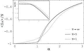
Figure 1: The behavior of $\langle S_{x}\rangle/N$ and of the ground state energy (inset) as a function of the parameter $\alpha$, for $D=10$. Different curves correspond to different values of $N$.

Numerical results for the ground state energy and the $x$-magnetization are plotted in Fig.(1) as a function of the parameter $\alpha$, for different values of $N$, in comparison with the results for $N\rightarrow\infty$.

In what follows, we will obtain an analytic expression for the $N$ dependence of $\Phi_{\nu}(ND)$, and, consequently, the scaling relations for all the observable introduced above.

Finite-size scaling exponents at the critical point.

In the adiabatic regime, i.e. for large $D$, the Schrödinger equation (10) can be approximately rewritten as

$$\left[-\frac{d^{2}}{dQ^{2}}+(\alpha_{c}-\alpha)Q^{2}+\frac{\alpha^{2}}{2ND}Q^{4}\right]\phi_{0}(Q;\alpha,ND)$$

$$=e_{0}(\alpha,ND)\,\phi_{0}(Q;\alpha,ND)$$ (20)

with $e_{0}(\alpha,ND)=E_{0}(\alpha,ND)+ND$, quartic .

Even thought the ground state energy and all of the physical observables appear to depend on the two parameters $\alpha$ and $ND$, this problem can be simplified in a single-parameter one with the help of Symanzik scaling simon , after transforming Eq. (Finite-size scaling exponents at the critical point.) into the equivalent form

$$\left[-\frac{d^{2}}{dq^{2}}+\zeta q^{2}+q^{4}\right]\phi_{0}(q;\zeta)=e_{0}\left(\zeta\right)\phi_{0}(q;\zeta)$$ (21)

where $q=Q\,\left(\frac{\alpha^{2}}{2ND}\right)^{1/6}$, while $\zeta=\left(\frac{2ND}{\alpha^{2}}\right)^{2/3}(\alpha_{c}-\alpha)$ is the only remaining scale parameter.

For the ground state energy one obtains the relation

$$E_{0}(\alpha,ND)=-ND+\left(\frac{\alpha^{2}}{2ND}\right)^{1/3}e_{0}\left(\zeta\right)\,.$$ (22)

Taking the limit $\alpha\rightarrow\alpha_{c}$ (or $\zeta\rightarrow 0$), Eq. (21) becomes

$$\left(-\frac{d^{2}}{dq^{2}}+q^{4}\right)\phi_{0}(q;0)=e_{0}(0)\phi_{0}(q;0)$$ (23)

whose lowest eigenvalue is found to be $e_{0}(0)\simeq 1.06036$. For $\zeta\neq 0$ (but near the critical point) we can resort to perturbation theory and obtain the ground state energy as an expansion in powers of $\zeta$,

$$e_{0}(\zeta)=\sum_{n=0}^{\infty}\beta_{n}\zeta^{n}\,.$$ (24)

It is easy to show that $\beta_{0}=e_{0}(0)$ and $\beta_{1}=\int_{-\infty}^{\infty}q^{2}\phi_{0}^{2}(q;0)dq=e_{0}^{\prime}(0)\simeq 0.36203$. We demonstrate below that these $\beta$’s enter not only the energy, but also the finite $N$ expansion of every physical observable.

In order to compute the average values listed in Eqs. (12-15) at the critical point, we expand the integral $\Phi_{\nu}(ND)$, given in Eq.(11), as

$$\Phi_{\nu}(ND)\simeq 1+\frac{2\alpha\nu}{ND}\langle Q^{2}\rangle+\frac{2\alpha^{2}(\nu-1)\nu}{N^{2}D^{2}}\langle Q^{4}\rangle$$ (25)

Taking the system energy $E_{0}(\alpha,ND)$ from Eq. (22), we exploit the Feynman-Hellman theorem to obtain

$$\frac{\partial E_{0}(\alpha,ND)}{\partial\alpha}=-\langle Q^{2}\rangle+\frac{\alpha}{ND}\langle Q^{4}\rangle\,,$$ (26)

$$\frac{\partial E_{0}(\alpha,ND)}{\partial(ND)}=-1-\frac{\alpha^{2}}{2N^{2}D^{2}}\langle Q^{4}\rangle\,.$$ (27)

Using Eq. (24), we get the critical point values

$$\langle Q^{2}\rangle={\beta_{1}}\left(2ND\right)^{1/3}\,,\quad\langle Q^{4}\rangle=\frac{\beta_{0}}{3}\left(2ND\right)^{2/3}\,$$ (28)

$$\Phi_{\nu}(ND)\simeq 1+\frac{4\nu}{(2ND)^{2/3}}\beta_{1}+\frac{8}{3}\frac{(\nu-1)\nu}{(2ND)^{4/3}}\beta_{0}\,.$$ (29)

Substituting into Eqs. (12)-(13), we have:

$$\frac{\langle S_{x}\rangle}{N}\simeq-1+\frac{2\beta_{1}}{(2ND)^{2/3}}-\frac{2\beta_{0}}{(2ND)^{4/3}}$$ (30)

$$\frac{\langle S_{x}^{2}\rangle}{N^{2}}\simeq 1-\frac{N-1}{N}\left[\frac{4\beta_{1}}{(2ND)^{2/3}}-\frac{16}{3}\frac{\beta_{0}}{(2ND)^{4/3}}\right]\,.$$ (31)

Finally, the order parameter is given by

$$\frac{\langle{P^{2}+Q^{2}}\rangle}{ND}\simeq\frac{2\beta_{1}}{(2ND)^{2/3}}+\frac{4}{3}\frac{\beta_{0}}{(2ND)^{4/3}}\,.$$ (32)

In Fig. (2) we make a comparison with the results obtained from the numerical solution of the Schrödinger equation (10). One can see that the leading finite size-corrections for $e_{0}/ND$ and ${\langle S_{x}\rangle}/{N}$ scale indeed as $N^{-4/3}$ and $N^{-2/3}$, respectively.

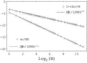
Figure 2: Scaling of the ground state energy and spin average as a function of $N$ at the critical point $\alpha=1$, for $D=10$.

When the system size is too small, the next to leading orders in these expansions become important and this explains the discrepancy with Ref.reslen , already pointed out in vidal .

The knowledge of $\beta_{0}$ and of the first two moments is sufficient to determine recursively all the others ($k\geq 2$):

$$\frac{\langle Q^{k+4}\rangle}{(2ND)^{2/3}}=\frac{k+1}{k+3}\beta_{0}\langle Q^{k}\rangle+\frac{k(k^{2}-1)}{4(k+3)}(2ND)^{1/3}\langle Q^{k+2}\rangle.$$ (33)

This relation allows one to compute higher order terms of the finite size expansion.

We conclude this part by pointing out that the oscillator state $\phi_{0}$ could also be found by a different re-scaling procedure, i.e. by rewriting the Hamiltonian as $H(\xi)=p^{2}+q^{2}+\xi q^{4}$ with $\xi=\alpha^{2}/2ND(\alpha_{c}-\alpha)^{3/2}$. In this case, however, the perturbation expansion would yield a power series that diverges very strongly for every $\xi\neq 0$. This would be the equivalent in our approach of the method of Ref.vidal , where the scaling exponents are obtained by arguing that there can be no singularity in any physical quantity at finite-size. Our leading order results agree with those reported in Ref.vidal except for the exponent of ${\langle S_{y}^{2}\rangle}/{N^{2}}$, on which we comment below.

Entanglement.

To start the discussion on quantum correlations in this model, we point out the peculiar nature of the adiabatic state of Eq. (3); namely, the fact that, once the oscillator is traced out, the $N$ qubits remain in a purely statistical mixture, without the presence of any entanglement, neither of pairwise, nor of multi-partite nature. In particular, the concurrence between any two qubits is zero. This is due to the adiabatic hypothesis $D\gg 1$, which strongly suppresses the energy exchange between qubits, mediated by the oscillator.

Since we obtain all the relevant features of the Dicke transition despite the fact that concurrence is neglected, we can conclude that its presence is not really essential to describe the large $N$ behavior. In fact, as reported by Ref. lambert2 , some degree of pairwise entanglement is present even in the regime $D\gg 1$ and therefore one should expect that the adiabatic approach fails in describing pairwise correlations. Interestingly enough, this is not entirely the case as, for large $N$, the only two-point correlation function for which we obtain a different scaling behavior is $\langle S_{y}^{2}\rangle$, and this difference is just enough to set the concurrence to zero.

As argued above, the quantum correlations that really matter for the phase transition are those involving the oscillator. Below, we evaluate i) the entanglement of each qubit with the rest of the system (as there is no entanglement among qubits, this is due to correlations with the boson mode), and ii) the amount of entanglement between the oscillator and the entire set of qubits.

After tracing out all of the other degrees of freedom, each qubit is found in the same state $\rho_{1}$, and participates of the entanglement (as measured by the tangle)

$$\tau_{1}=2\Bigl{[}1-\mbox{Tr}\rho_{1}^{2}\Bigr{]}\equiv 1-\frac{\langle S_{x}\rangle^{2}}{N^{2}}\,.$$ (34)

In the thermodynamic limit, this is zero in the normal phase, while one gets $\tau_{1}=1-\frac{1}{\alpha^{2}}$ for $\alpha>1$. For large but finite $N$, $\tau_{1}$ is non-zero even for $\alpha\leq 1$; but at the critical point it scales as $\tau_{1}\simeq\frac{4\beta_{1}}{(2ND)^{2/3}}$.

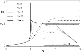
Figure 3: The tangle $\tau_{N}$ between the oscillator and the $N$ qubits as a function of $\alpha$, for $D=10$ and different values of $N$. The inset shows the scaling of $\tau_{N}$ with $N$ at $\alpha=\alpha_{c}=1$, compared with the analytic expression of Eq. (38) (continuous plot).

We adopt the linear entropy also to quantify the entanglement between the oscillator and the $N$ qubits. Thus

$$\tau_{N}=\eta\Bigl{(}1-\mbox{Tr}\left\{\rho_{N}^{2}\right\}\Bigr{)}\,,$$ (35)

where $\rho_{N}=\mbox{Tr}_{osc}|\psi\rangle\langle\psi|$ is the reduced qubit state, while the pre-factor is chosen to be $\eta=\frac{2^{N}}{2^{N}-1}$ to bound $\tau_{N}$ to $1$, see Ref. scott . Explicitly, we have

$$\mbox{Tr}\rho_{N}^{2}=\int dQdQ^{\prime}\,\phi_{0}^{2}(Q)\phi_{0}^{2}(Q^{\prime})\Bigl{[}1+\frac{\Theta^{2}(\sqrt{QQ^{\prime}})}{\Theta(Q)\,\Theta(Q^{\prime})}\Bigr{]}^{N}$$ (36)

which can be expressed as a power series in $\Phi_{\nu}$.

Fig. (3) shows $\tau_{N}$ both for finite $N$ and for $N\rightarrow\infty$. In the thermodynamic limit, we find

$$\tau_{\infty}=\left\{\begin{array}[]{ll}1-\left(1+\frac{\alpha}{D\sqrt{1-\alpha}}\right)^{-\frac{1}{2}}&\hbox{$(\alpha\leq 1)$}\\ 1-\frac{1}{2}\left(1+\frac{1}{D\alpha^{2}\sqrt{\alpha^{2}-1}}\right)^{-\frac{1}{2}}&\hbox{$(\alpha>1),$}\\ \end{array}\right.\,,$$ (37)

which shows a cusp at the critical point, where $\tau_{\infty}=1$. For finite $N$, this singular behavior is rounded and $\tau$ is quenched. When $N$ is large, the entanglement scales as

$$\tau_{N}(\alpha=\alpha_{c})\sim 1-\,\frac{\sqrt{\pi}\,K}{(2D)^{1/3}N^{1/6}}\,,$$ (38)

where $K=\int dq\phi_{0}^{4}(q;0)\simeq 0.46$, and $\phi_{0}(q;0)$ is the normalized solution of Eq. (23). This result is shown in Fig. (3) to agree with the numerical evaluation of Eq. (35).

To summarize, we have described the finite size scaling of quantum correlations in the Dicke model, obtaining the finite $N$ behavior of the spin components, of the order parameter and of the ground state entanglement in the adiabatic regime $D\gg 1$. We also discussed the crucial role of the entanglement involving the oscillator at criticality, giving its expression both in the thermodynamic limit and for a finite size system.

References

- (1) A.Osterloh et al., Nature (London) 416, 608 (2002).
- (2) G. Vidal, J. I. Latorre, E. Rico and A. Kitaev, Phys. Rev. Lett. 90, 227902 (2003).
- (3) L.-A. Wu, M.S. Sarandy and D.A. Lidar, Phys. Rev. Lett. 93, 250404 (2004).
- (4) R.H. Dicke, Phys. Rev. 93, 99 (1954).
- (5) K. Hepp and E. Lieb, Ann. Phys. 76 (1973) 360.
- (6) Y.K. Wang and F.T. Hioe, Phys. Rev. A 7, 831 (1973).
- (7) R. Gilmore and C.M. Bowden, Phys. Rev. A 13, 1898 (1976).
- (8) G. Liberti and R.L. Zaffino, Phys. Rev. A 70, 033808 (2004); Eur. Phys. J. B 44, 535 (2005).
- (9) T. Brandes, Phys. Rep. 408, 315 (2005).
- (10) S. Schneider and G.J. Milburn, Phys. Rev. A 65, 042107 (2002).
- (11) C. Emary and T. Brandes, Phys. Rev. Lett. 90 (2003) 044101; Phys. Rev. E 67, 066203 (2003).
- (12) X.W. Hou and B. Hu, Phys. Rev. A 69, 042110 (2004).
- (13) V. Bužek, M. Orszag and M. Rosko, Phys. Rev. Lett. 94, 163601 (2005).
- (14) N. Lambert, C. Emary and T. Brandes, Phys. Rev. Lett. 92, 073602 (2004).
- (15) N. Lambert, C. Emary and T. Brandes, Phys. Rev. A 71, 053804 (2005).
- (16) J. Reslen, L. Quiroga and N.F. Johnson, et al., Europhys. Lett. 69, 8 (2005).
- (17) J. Vidal and S. Dusuel, cond-mat/0510281.
- (18) G. Liberti et al., Phys. Rev. A 73, 032346 (2006).
- (19) C.M. Bender and T.T. Wu, Phys. Rev. D 7, 1620 (1973); W. Janke and H. Kleinert, Phys. Rev. Lett. 75, 2787 (1995).
- (20) B. Simon and A. Dicke, Ann. Phys. 58, 76 (1970).
- (21) A. J. Scott, Phys. Rev. A 69, 052330 (2004).