Entanglement of Dirac fields in non-inertial frames

Abstract

We analyze the entanglement between two modes of a free Dirac field as seen by two relatively accelerated parties. The entanglement is degraded by the Unruh effect and asymptotically reaches a non-vanishing minimum value in the infinite acceleration limit. This means that the state always remains entangled to a degree and can be used in quantum information tasks, such as teleportation, between parties in relative uniform acceleration. We analyze our results from the point of view afforded by the phenomenon of entanglement sharing and in terms of recent results in the area of multi-qubit complementarity.

I Introduction

Entanglement plays a central role in quantum information theory. It is considered a resource for quantum communication and teleportation, as well as for various computational tasks ekertbook . The importance of understanding entanglement in a relativistic setting has received considerable attention recently allthespecials ; teleport ; ivette ; ball . Such an understanding is certainly relevant from a fundamental point of view, since relativity is an indispensable component of any complete theoretical model. However, it is also important in a number of practical situations, for example, when considering the implementation of quantum information processing tasks performed by observers in arbitrary relative motion.

Entanglement was shown to be an invariant quantity for observers in uniform relative motion in the sense that, although different inertial observers may see these correlations distributed among several degrees of freedom in different ways, the total amount of entanglement is the same in all inertial frames allthespecials . In non-inertial frames, entanglement was first studied indirectly by investigating the fidelity of teleportation between two parties in relative uniform acceleration teleport . More recently, the observer-dependent character of entanglement was explicitly demonstrated by studying the entanglement between two modes of a free scalar field as viewed by two relatively accelerated observers ivette .

A uniformly accelerated observer is unable to access information about the whole of spacetime since, from his perspective, a communication horizon appears. This can result in a loss of information and a corresponding degradation of entanglement. In essence, the acceleration of the observer effects a kind of “enviromental decoherence”, limiting the fidelity of certain quantum information-theoretic processes. A quantitative understanding of such degradation in non-inertial frames is therefore required if one wants to discuss the implementation of certain quantum information processing tasks between accelerated partners.

In curved spacetime two nearby inertial observers are relatively accelerated due to the geodesic deviation equation. Accordingly, the results of ivette indicate that in curved spacetime even two inertial observers will disagree on the degree of entanglement in a given bipartite quantum state of some quantum field. Indeed, a thorough investigation into entanglement in an expanding curved spacetime shows that entanglement can encode information concerning the underlying spacetime structure ball .

In this paper we analyze the entanglement between two modes of a Dirac field described by relatively accelerated parties in a flat spacetime. We are interested in understanding how both the crucial sign change in Fermi-Dirac versus Bose-Einstein distributions, and the finite number of allowed states in fermionic systems due to the Pauli exclusion principle (in contrast to the unbounded excitations that can occur in bosonic systems), affect the degradation of entanglement produced by the Unruh effect. We find that unlike the bosonic case, where the entanglement degrades completely in the infinite acceleration limit, in the fermionic case the entanglement is never completely destroyed. We analyze the degradation of entanglement in the system by applying the constraints of entanglement sharing Coffman and track the information originally encoded in these quantum correlations by employing a set of multi-qubit complementarity relations Tessier . As in ivette , our results can be applied to the case that Alice falls into a black hole whilst Rob barely escapes through eternal uniform acceleration.

The remainder of this paper is organized as follows. In Sec. II we consider two modes of a free Dirac field that are maximally entangled from an inertial perspective. Two parties, an inertial observer named Alice and a uniformly accelerating observer named Rob, are each assumed to possess a detector sensitive only to one of the two modes. Each measures the field with his/her detector and the results are compared in order to estimate the entanglement between the modes.

Section III discusses the Unruh effect for Dirac particles as experienced by Rob. If a given Dirac mode is in the vacuum state from an inertial perspective, then Rob’s detector perceives a Fermi-Dirac distribution of particles. This has a strong effect on the entanglement that exists between Alice and Rob, and therefore plays an important role in any quantum information task they might perform that uses this entanglement as a resource.

In Sec. IV we calculate the entanglement between the modes from the perspectives of both Alice and Rob. Due to the presence of a Rindler horizon, Rob is forced to trace over a causally disconnected region of spacetime that he cannot access. Accordingly, his description of the system takes the form of a two-qubit mixed state. We calculate the entanglement using mixed state entanglement measures such as the entanglement of formation formation and the logarithmic negativity negativity . We also estimate the total correlations (classical plus quantum) via the mutual information mutual . Our results show that the entanglement of formation does not vanish as it does in the bosonic case, but rather reaches a minimum of $1/\sqrt{2}$ in the limit that Rob moves with infinite acceleration.

Since the fermionic system we are considering is accurately described by a pure state of three qubits, we study the constraints placed on the system by the phenomenon of entanglement sharing in Sec. V. Our analysis shows that no inherently three-body correlations are generated in the quantum state. That is, all of the entanglement in the system is in the form of bipartite correlations, regardless of Rob’s rate of acceleration.

Using complementarity relations applicable to an overall pure state of three qubits, as well as to the various two-qubit marginals, we identify the different types of information encoded in the quantum state of our system in Sec. VI. This enables us to study how specific subsystem properties depend on Rob’s rate of acceleration and to explain how some of the entanglement from the inertial frame is able to survive in the fermionic system, even at infinite acceleration. Finally, we summarize our results and suggest possible directions for further research in Sec. VII.

II The setting

Consider a free Minkowski Dirac field in $3+1$ dimensions

$$i\gamma^{\mu}\partial_{\mu}{\psi}-m\psi=0,$$

where $m$ is the particle mass, $\gamma^{\mu}$ the Dirac gamma matrices, and $\psi$ is a spinor wavefunction. Minkowski coordinates $x^{\mu}=(ct,\mathbf{x})$ with $\mu=\{0,1,2,3\}$ are the most suitable to describe the field from an inertial perspective. The field can be expanded in terms of the positive (fermions) and negative (antifermions) energy solutions of the Dirac equation $\psi_{k}^{+}$ and $\psi_{k}^{-}$ respectively, since they form a complete orthonormal set of modes,

$$\psi=\int dk\,(a_{k}\psi_{k}^{+}+b_{k}^{\dagger}\psi_{k}^{-}).$$ (1)

In the above, $k$ is a notational shorthand for the wavevector $\mathbf{k}$ which labels the modes. The positive and negative energy Minkowski modes have the form

$$\left(\psi_{k}^{\pm}\right)_{s}=\frac{1}{\sqrt{2\pi\omega_{k}}}\,\phi^{\pm}_{s}\,e^{\pm i(\mathbf{k}\cdot\mathbf{x}-\omega_{k}t)},$$

where $\omega_{k}=(m^{2}+\mathbf{k}^{2})^{1/2}$, and $\phi_{s}=\phi_{s}(\mathbf{k})$ is a constant spinor with $s=\{\uparrow,\downarrow\}$ indicating spin-up or spin-down along the quantization axis, satisfying the normalization relations mandl_shaw $\pm\bar{\phi}^{\pm}_{s}\,\phi^{\pm}_{s^{\prime}}=(\omega_{k}/m)\,\delta_{ss^{\prime}}$, $\bar{\phi}^{\pm}_{s^{\prime}}\,\phi^{\mp}_{s^{\prime}}=0$, with the adjoint spinor given by $\bar{\phi}^{\pm}_{s}=\phi^{\pm\dagger}_{s}\,\gamma^{0}$. The above positive and negative energy solutions satisfy the orthogonormality relations

$$(\psi_{k}^{+},\psi_{k^{\prime}}^{+})=-(\psi_{k}^{-},\psi_{k^{\prime}}^{-})=\delta(k-k^{\prime}),\quad(\psi_{k}^{\pm},\psi_{k^{\prime}}^{\mp})=0,$$

where the Dirac inner product for two mode functions is given by

$$\big{(}\phi(\mbox{{\boldmath$x$}},t),\varphi(\mbox{{\boldmath$x$}},t)\big{)}=\int\,d\mbox{{\boldmath$x$}}\,\phi^{\dagger}(\mathbf{x},t)\,\varphi(\mathbf{x},t).$$

The modes $\psi_{k}^{\pm}$ are classified as positive and negative frequency with respect to (the future-directed Minkowski Killing vector) $\partial_{t}$ for $\omega_{k}>0$, i.e.

$$\partial_{t}\,\psi_{k}^{\pm}=\mp\,i\,\omega_{k}\,\psi_{k}^{\pm},\qquad\omega_{k}>0.$$

The operators $a_{k}^{\dagger},b_{k}^{\dagger}$ and $a_{k},b_{k}$ are the creation and annihilation operators for the positive and negative energy solutions of momentum $k$ which satisfy the anticonmutation relations

$$\{a_{i},a_{j}^{\dagger}\}=\{b_{i},b_{j}^{\dagger}\}=\delta_{ij},$$

with all other anticommutators vanishing. The Minkowski vacuum state is defined by the absence of any mode excitations in an inertial frame,

$$|0\rangle=\prod_{kk^{\prime}}|0_{k}\rangle^{+}|0_{k^{\prime}}\rangle^{-},$$

where the $\{+,-\}$ superscript on the kets is used to indicate the particle and anti-particle vacua, respectively so that $a_{k}|0_{k}\rangle^{+}=b_{k}|0_{k}\rangle^{-}=0$. We will use the notation here, and throughout the rest of the work, that the mode index ($k,k^{\prime}\ldots$) will be a subscript affixed to the occupation number inside the ket, and that the absence of a subscript on the outside of the ket indicates a Minkowski Fock state. Since $(a_{k}^{\dagger})^{2}=(b_{k}^{\dagger})^{2}=0$, there are only two allowed states for each mode, $|0_{k}\rangle^{+}$ and $|1_{k}\rangle^{+}=a_{k}^{\dagger}|0_{k}\rangle^{+}$ for particles, and similarly for anti-particles.

Consider two maximally entangled fermionic modes in an inertial frame,

$$|\phi_{k_{A},k_{R}}\rangle=\frac{1}{\sqrt{2}}(|0_{k_{A}}\rangle^{+}|0_{k_{R}}\rangle^{+}+|1_{k_{A}}\rangle^{+}|1_{k_{R}}\rangle^{+}),$$ (2)

where the subscripts $A$ and $R$ indicate the modes associated with the observers Alice and Rob, respectively. All other modes of the field are in the vacuum state, and therefore the state can be written as $|\Phi\rangle=|\phi_{k_{A},k_{R}}\rangle\,\{\prod_{k\neq k_{A},k_{R}}|0_{k}\rangle^{+}\prod_{k^{\prime}}|0_{k^{\prime}}\rangle^{-}\}$. Now assume that Alice is stationary and has a detector sensitive only to mode $k_{A}$. Rob moves with uniform acceleration and takes with him a detector that only detects particles corresponding to mode $k_{R}$. We ask the question of what is the entanglement between modes $k_{A}$ and $k_{R}$ observed by Alice and Rob, given that Rob undergoes uniform acceleration. Note that in order to determine the amount of entanglement, Alice and Rob perform measurements which are then compared by either party in order to estimate the correlations in the results. Due to Rob’s acceleration, at some point Alice’s signals will no longer reach Rob, but Rob’s signals will always be available to Alice, (see Fig. 1). At this point only Alice can compare the measurement results and estimate the entanglement of the state. Let us now consider the state observed by Rob.

III Unruh effect for Dirac particles

Consider Rob to be uniformly accelerated in the $(t,z)$ plane ($c=1$). Rindler coordinates $(\tau,\zeta)$ are appropriate for describing the viewpoint of an observer moving with uniform acceleration. Two different sets of Rindler coordinates, which differ from each other by an overall change in sign, are necessary for covering Minkowski space note1 . These sets of coordinates define two Rindler regions that are causally disconnected from each other.

$$at = \hskip 5.0pte^{a\zeta}\sinh(a\tau),\quad az=\hskip 5.0pte^{a\zeta}\cosh(a\tau),\hskip 5.0pt\textrm{in region I}$$

$$at = -e^{a\zeta}\sinh(a\tau),\quad az=-e^{a\zeta}\cosh(a\tau),\hskip 2.5pt\textrm{in region II}$$

where $a$ denotes Rob’s proper acceleration. The above set of coordinates both give rise to the same Rindler metric

$$ds^{2}=dt^{2}-dz^{2}-d^{2}\mathbf{x}_{\perp}=e^{2a\zeta}\left(d^{2}\tau-d^{2}\zeta\right)-d^{2}\mathbf{x}_{\perp},$$

where $\mathbf{x}_{\perp}=(x,y)$ are the same in both Minkowski and Rindler spacetimes.

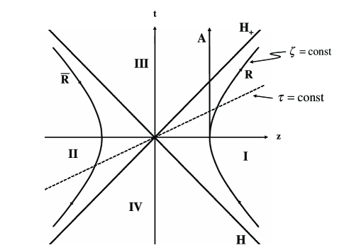
Figure 1: Rindler spacetime diagram: Lines of constant position $\zeta$ are hyperbolas and lines of constant proper time $\tau$ for the accelerated observer run through the origin. Note that while $\tau$ flows in the direction of $t$ in region I, it flows in the direction of $-t$ in region II, (i.e the dashed line rotates counter-clockwise for increasing values of $\tau$). A uniformly accelerated observer Rob ($R$) with acceleration $a$ travels on a hyperbola constrained to region I, while a fictitious observer anti-Rob $(\bar{R})$ travels on a corresponding hyperbola in region II given by the negative of Rob’s coordinates. The horizons $H_{\pm}$ are lines of $\tau=\pm\infty$ which Alice ($A$) will cross at finite Minkowski times.

A particle undergoing eternal uniform acceleration remains constrained to either Rindler region I or II and has no access to the opposite region, since these two regions are causally disconnected. Figure 1 serves to illustrate these ideas, as well as to introduce our labeling scheme, where we refer to the accelerated observer in region I as Rob (R) and to the corresponding fictitious observer confined to region II (whose coordinates are the negative of Rob’s) as anti-Rob $\left(\rm{\bar{R}}\right)$.

The coordinates $(\tau,\zeta)$ have the ranges $-\infty<\tau,\,\zeta<\infty$ separately in region I and in region II. This implies that region I and II each admit a separate quantization procedure with corresponding positive and negative energy solutions $\{\psi^{I+}_{k},\psi^{I-}_{k}\}$ and $\{\psi^{II+}_{k},\psi^{II-}_{k}\}$. Since the Rindler metric is static (independent of $\tau$) it will admit solutions of the form $e^{-i\omega\tau}\,\phi_{\alpha}(\zeta,\mathbf{x}_{\perp})$, with $\phi_{\alpha}$ a spatially dependent spinor note_on_spin . Particles and anti-particles will be classified with respect to the future-directed timelike Killing vector in each region. In region I this is given by $\partial_{\tau}$ where

$$\partial_{\tau}=\frac{\partial t}{\partial\tau}\,\partial_{t}+\frac{\partial z}{\partial\tau}\,\partial_{z}=a\,(z\partial_{t}+t\partial_{z}),$$

which is a boost into the instantaneous comoving frame of Rob. Thus, mode solutions in region I having time dependence $\psi^{I+}_{k}\sim e^{-i\omega\tau}$ with $\omega>0$ represent positive frequency solutions since $\partial_{\tau}\psi^{I+}_{k}=-i\omega\psi^{I+}_{k}$. However, in region II $\partial_{\tau}$ points in the opposite direction of $\partial_{t}$ (increasing $\tau$ flows in the direction of $-t$, see Fig. 1). Hence in region II the future-directed timelike Killing vector is given by $\partial_{-\tau}=-\partial_{\tau}$ BD ; carroll . Thus, a solution in region II with time dependence $e^{-i\omega\tau}$ with $\omega>0$ is actually a negative frequency mode since $\partial_{-\tau}\,e^{-i\omega\tau}=i\omega\,e^{-i\omega\tau}$. Hence, the positive frequency mode in region II is given by $\psi^{II+}_{k}\sim e^{i\omega\tau}$ with $\omega>0$ satisfying $\partial_{-\tau}\psi^{II+}_{k}=-i\omega\psi^{II+}_{k}$. Due to the causally disjoint nature of region I and II, the modes $\psi^{I\pm}_{k}$ have support only in region I and vanish in region II, while the opposite is true for the modes $\psi^{II\pm}_{k}$ in region II. The Rindler modes satisfy orthonormality relations analogous to the Minkowski modes note2 $(\psi^{\sigma\pm}_{k},\psi^{\sigma^{\prime}\mp}_{k^{\prime}})=0$, and $(\psi^{\sigma\pm}_{k},\psi^{\sigma^{\prime}\pm}_{k^{\prime}})=\pm\,\delta_{\sigma,\sigma^{\prime}}\,\delta(k-k^{\prime})$ where $\sigma\in\{I,II\}$.

In region I, let us denote $(c_{k}^{I},c^{I\dagger}_{k})$ as the annihilation and creation operators for fermions (particles) and $(d_{k}^{I},d^{I\dagger}_{k})$ as the annihilation and creation operators for anti-fermions (anti-particles). The corresponding particle and anti-particle operators in region II are denoted as $(c_{k}^{II},c^{II\dagger}_{k})$ and $(d_{k}^{II},d^{II\dagger}_{k})$. These obey the usual Dirac anti-commutation relations $\{c_{k}^{\sigma},c^{\sigma^{\prime}\dagger}_{k^{\prime}}\}=$ $\{d_{k}^{\sigma},d^{\sigma^{\prime}\dagger}_{k^{\prime}}\}=$ $\delta_{\sigma\sigma^{\prime}}\,\delta_{kk^{\prime}}$, with all other anti-commutators, including those between operators in region I and the causally disconnected region II, equaling zero. Taking into account the two sets of modes in each Rindler region, the Dirac field can be expanded, in analogy to Eq. (1), as

$$\psi=\int dk\left(c_{k}^{I}\psi_{k}^{I+}+d_{k}^{I\dagger}\psi_{k}^{I-}+c_{k}^{II}\psi_{k}^{II+}+d_{k}^{II\dagger}\psi_{k}^{II-}\right).$$ (4)

Eq. (1) and Eq. (4) represent the decomposition of the Dirac field in Minkowski and Rindler modes, respectively. We can therefore relate the Minkowski and Rindler creation and annihilation operators by taking appropriate inner products. Using the Rindler orthogonality relations and Eq. (4) we have $c^{\sigma}_{k}=(\psi^{\sigma+}_{k},\psi)$. Substituting Eq. (1) for $\psi$ in this last expression yields

$$c^{\sigma}_{k}=\int dk^{\prime}\,\left(\alpha^{\sigma}_{kk^{\prime}}\,a_{k^{\prime}}+\beta^{\sigma}_{kk^{\prime}}\,b^{\dagger}_{k^{\prime}}\right),\quad\sigma\in\{I,II\}$$ (5)

where the Bogoliubov coefficients are given by the inner product of the Rindler modes wavefunctions with the Minkowski positive and negative frequency modes

$$\alpha^{\sigma}_{kk^{\prime}}=\left(\psi^{\sigma+}_{k},\psi^{+}_{k^{\prime}}\right),\qquad\beta^{\sigma}_{kk^{\prime}}=\left(\psi^{\sigma+}_{k},\psi^{-}_{k^{\prime}}\right).$$ (6)

A similar calculation for $d^{\sigma}_{k}$ yields the corresponding expression

$$d^{\sigma}_{k}=\int dk^{\prime}\,\left(\alpha^{\sigma}_{kk^{\prime}}\,b_{k^{\prime}}+\beta^{\sigma}_{kk^{\prime}}\,a^{\dagger}_{k^{\prime}}\right),\quad\sigma\in\{I,II\}$$ (7)

with the same Bogoliubov coefficient as in Eq. (6). In deriving Eq. (7) use has been made of the following properties of the Dirac inner product: $(\phi_{1},\phi_{2})^{*}=(\phi_{1}^{*},\phi_{2}^{*})=(\phi_{2},\phi_{1})$. The calculation of the Bogoliubov coefficients is straightforward, though lengthy and an exercise in special functions. Details can be found elsewhere takagi ; rocio ; mcmahon_alsing_embid . For our purposes, the end result of such calculations yields a relationship between the Minkowski and Rindler creation and annihilation operators given by the Bogoliubov transformation

$$\left[\begin{array}[]{c}a_{k}\\ b_{-k}^{\dagger}\\ \end{array}\right]=\left[\begin{array}[]{cc}\cos r&-e^{-i\phi}\,\sin r\\ e^{i\phi}\,\sin r&\cos r\\ \end{array}\right]\,\left[\begin{array}[]{c}c^{I}_{k}\\ d^{II\dagger}_{-k}\\ \end{array}\right],$$ (14)

where $\tan r=\exp(-\pi\Omega)$ with $\Omega\equiv\omega/(a/c)$, the ratio of the frequency $\omega$ to the only naturally occurring frequency in the problem $a/c$, and $\phi$ is an unimportant phase that can always be absorbed into the definition of the operators. It is easy to see from Eq. (14) and its adjoint that given the anti-commutation relations of the Rindler operators, the Minkowski anti-commutation relations are preserved. In Eq. (14) we have made the single mode approximation teleport , which is valid if we consider Rob’s detector as sensitive to a single particle mode in region I such that we can approximate the frequency $\omega_{A}$ observed by Alice to be the same as the frequency $\omega_{R}$ as observed by Rob, i.e $\omega_{A}\sim\omega_{R}=\omega$ note2.5 . Note that this Bogoliubov transformation mixes a particle in region I and an anti-particle in region II. Correspondingly, the Bogoliubov transformation that mixes an anti-particle mode in region I and a particle in region II is given by

$$\left[\begin{array}[]{c}b_{k}\\ a_{-k}^{\dagger}\\ \end{array}\right]=\left[\begin{array}[]{cc}\cos r&e^{-i\phi}\,\sin r\\ -e^{-i\phi}\,\sin r&\cos r\\ \end{array}\right]\,\left[\begin{array}[]{c}d^{I}_{k}\\ c^{II\dagger}_{-k}\\ \end{array}\right].$$ (21)

Since the anti-commutators between particle and anti-particle operators and between region I and region II Rindler operators are zero, it is easy to see that the Minkowski operators in Eq. (14) anti-commute with the Minkowski operators in Eq. (21), as they should (since $k$ and $-k$ represent two separate modes).

As stated above, Eq. (14) reveals that the Minkowski particle annihilation operator is a Bogoliubov transformation between a particle in region I of momentum $k$ and an anti-particle in region II of momentum $-k$, i.e. a transformation that mixes creation and annihilation operators. We can understand this in terms of our previous discussion of the time dependence of positive frequency Rindler modes in regions I and II. For a massless Dirac field a positive frequency Rindler mode has the form mcmahon_alsing_embid $\psi^{I+}_{k}\sim\exp(ik\zeta-i\omega\tau)$ (for the scalar case see carroll ; takagi ) and a positive frequency Rindler mode in region II has the form $\psi^{II+}_{k}\sim\exp(ik\zeta+i\omega\tau)$. Thus, in order to construct a positive frequency Minkowski mode $\psi^{+}$ that extends $\psi^{I+}_{k}$ analytically from region I to region II, we need a linear combination of $\psi^{I+}_{k}$ and $(\psi^{II+}_{-k})^{*}$ so that both have the space and time dependence $\exp(ik\zeta-i\omega\tau)$. This means that the Minkowski operator $a_{k}$ must mix $c^{I}_{k}$ and $d^{II\dagger}_{-k}$ as in Eq. (14). Similarly, to construct a Minkowski mode that analytically extends $\psi^{II+}_{k}$ from region II to region I we must form a linear combination of $\psi^{II+}_{k}$ and $(\psi^{I-}_{-k})^{*}$ so that both have the space and time dependence $\exp(ik\zeta+i\omega\tau)$. This corresponds to $b_{k}$ mixing $d^{I}_{k}$ and $c^{II\dagger}_{-k}$ as in Eq. (21). For a massive Dirac field the time dependence of the Rindler modes remains the same, but the spatial dependence is more complicated mcmahon_alsing_embid . The above argument for the mixing of Rindler particles (anti-particles) in region I (II) and anti-particles (particles) in region II (I) goes through unchanged.

Having related Minkowski and Rindler creation and annihilation operators, we now wish to relate the Minkowski vacuum to the corresponding Rindler vacuum. It is useful to note that Eq. (14) can be written as a two-mode squeezing transformation milburn_walls

$$\left[\begin{array}[]{c}a_{k}\\ b_{-k}^{\dagger}\\ \end{array}\right]=S\,\left[\begin{array}[]{c}c^{I}_{k}\\ d^{II\dagger}_{-k}\\ \end{array}\right]\,S^{\dagger}$$

for the single mode $k$ with $S$ given by

$$S=\exp\left[r\,\left(c^{I\dagger}_{k}\,d^{II\dagger}_{-k}\,e^{-i\phi}+c^{I}_{k}\,d^{II}_{-k}\,e^{i\phi}\right)\right].$$

Using the relation $e^{A}\,B\,e^{-A}=B+[B,A]+[B,[B,A]]/2!+[B,[B,[B,A]]]/3!+\cdots$ and the identity $[AB,C]=A\,\{B,C\}-\{A,C\}\,B$ we find

$$a_{k} = Sc^{I}_{k}S^{\dagger}=c^{I}_{k}-re^{-i\phi}\,d^{II\dagger}_{-k}-\frac{r^{2}}{2!}\,c^{I}_{k}+\frac{r^{3}}{3!}\,e^{-i\phi}\,d^{II\dagger}_{-k}+\cdots$$ (22)

$$= \cos r\,c^{I}_{k}-e^{-i\phi}\sin r\,d^{II\dagger}_{-k}.$$

and

$$b^{\dagger}_{-k} = Sd^{II\dagger}_{-k}S^{\dagger}=d^{II\dagger}_{-k}+re^{i\phi}\,c^{I}_{k}-\frac{r^{2}}{2!}\,d^{II\dagger}_{-k}-\frac{r^{3}}{3!}\,e^{i\phi}\,c^{I}_{k}+\cdots$$ (23)

$$= \cos r\,d^{II\dagger}_{-k}+e^{-i\phi}\sin r\,c^{I}_{k}.$$

Now $a_{k}$ and $b_{-k}$, respectively, annihilate the single mode particle and anti-particle Minkowski vacua $a_{k}|0_{k}\rangle^{+}=0$ and $b_{-k}|0_{-k}\rangle^{-}=0$. Since $a_{k}$ mixes particles in region I and anti-particles in region II, we postulate that the Minkowski particle vacuum for mode $k$ in terms of Rindler Fock states is given by

$$|0_{k}\rangle^{+}=\sum_{n=0}^{1}A_{n}\,|n_{k}\rangle^{+}_{I}\,|n_{-k}\rangle^{-}_{II},$$ (24)

where note3

$$\begin{array}[]{lll}c^{I}_{k}|0_{k}\rangle^{+}_{I}=0&&d^{II}_{-k}|0_{-k}\rangle^{-}_{II}=0,\\ &&\\ c^{I\dagger}_{k}|0_{k}\rangle^{+}_{I}=|1_{k}\rangle^{+}_{I}&&d^{II\dagger}_{-k}|0_{-k}\rangle^{-}_{II}=|1_{-k}\rangle^{-}_{II}.\\ \end{array}$$ (25)

As a comment on notation, the Rindler region I and II Fock states carry a subscript I or II, respectively, on the kets while the Minkowski Fock states are indicated by the absence of an outside subscript on the kets. Momentum mode labels are attached to the Fock occupation number, and the $\{+,-\}$ ket superscript indicates a particle or anti-particle state, respectively. Applying $a_{k}$ from Eq. (22) to Eq. (24), we have

$$0 = a_{k}|0_{k}\rangle^{+}$$ (26)

$$= \left(\cos r\,c^{I}_{k}-e^{-i\phi}\sin r\,d^{II\dagger}_{-k}\right)\,\sum_{n=0}^{1}A_{n}\,|n_{k}\rangle^{+}_{I}\,|n_{-k}\rangle^{-}_{II}$$

$$= (A_{1}\,\cos r-A_{0}\,e^{-i\phi}\,\sin r)\,|0_{k}\rangle^{+}_{I}\,|1_{-k}\rangle^{-}_{II}$$

$$\Rightarrow A_{1}=A_{0}\,e^{-i\phi}\,\tan r.$$

Normalization ${}^{+}\langle 0_{k}|0_{k}\rangle^{+}=$ $|A_{0}|^{2}+|A_{1}|^{2}=1$ yields $A_{0}=\cos r$ so that we finally arrive at

$$|0_{k}\rangle^{+} = \cos r\,|0_{k}\rangle^{+}_{I}\,|0_{-k}\rangle^{-}_{II}+e^{-i\phi}\,\sin r\,|1_{k}\rangle^{+}_{I}\,|1_{-k}\rangle^{-}_{II},$$ (27)

$$= \left[\cos r\,+e^{-i\phi}\,\sin r\,c^{I\dagger}_{k}\,d^{II\dagger}_{-k}\right]\,|0_{k}\rangle^{+}_{I}\,|0_{-k}\rangle^{-}_{II},$$

where the second equality in Eq. (27) is very useful for keeping track of any possible transposition signs arising from the anti-commuting operators when applying Minkowski operators to $|0_{k}\rangle^{+}$. As an important example that we will use subsequently, a short calculation of $a_{k}^{\dagger}\,|0_{k}\rangle^{+}$ using the adjoint of Eq. (22)

$$a_{k}^{\dagger}=\cos r\,c^{I\dagger}_{k}-e^{+i\phi}\sin r\,d^{II}_{-k},$$ (28)

acting on the lower expression for $|0_{k}\rangle^{+}$ in Eq. (27), yields

$$a_{k}^{\dagger}\,|0_{k}\rangle^{+} = \left(\cos^{2}r\,c^{I\dagger}_{k}-\sin^{2}r\,d^{II}_{-k}\,c^{I\dagger}_{k}\,d^{II\dagger}_{-k}\right)\,\,|0_{k}\rangle^{+}_{I}\,|0_{-k}\rangle^{-}_{II},$$

$$= \left(\cos^{2}r\,c^{I\dagger}_{k}+\sin^{2}r\,c^{I\dagger}_{k}\,d^{II}_{-k}\,d^{II\dagger}_{-k},\right)\,\,|0_{k}\rangle^{+}_{I}\,|0_{-k}\rangle^{-}_{II}$$

$$= c^{I\dagger}_{k}\,|0_{k}\rangle^{+}_{I}\,|0_{-k}\rangle^{-}_{II},$$

$$|1_{k}\rangle^{+} = |1_{k}\rangle^{+}_{I}\,|0_{-k}\rangle^{-}_{II}.$$ (29)

where in the second equality we have used the anti-commutation relations between $c^{I\dagger}_{k}$ and $d^{II}_{-k}$ to obtain a minus sign upon transposition, and in the third equality we have used the anti-commutation relations to write $d^{II}_{-k}\,d^{II\dagger}_{-k}=1-d^{II\dagger}_{-k}\,d^{II}_{-k}$, noting that the latter term annihilates the anti-particle vacuum. Lastly, one can easily verify that $a_{k}^{\dagger}$ acting on $|1_{k}\rangle^{+}$ yields zero,

$$a_{k}^{\dagger}|1_{k}\rangle^{+}=\left(\cos r\,c^{I\dagger}_{k}-e^{+i\phi}\sin r\,d^{II}_{-k}\right)\,|1_{k}\rangle^{+}_{I}\,|0_{-k}\rangle^{-}_{II}=0,$$ (30)

ensuring that $(a_{k}^{\dagger})^{2}=0$.

We note that the form of the Dirac particle vacuum for mode $k$ in Eq. (27), which can be written as $|0_{k}\rangle^{+}=\cos r\sum_{n=0}^{1}\tan^{n}r\,|n_{k}\rangle^{+}_{I}\,|n_{-k}\rangle^{-}_{II}$, is complementary to the form of the Minkowski charged scalar vacuum for mode $k$, which is given by teleport ; takagi

$$|0_{k}\rangle^{+}=(\cosh r)^{-1}\sum_{n=0}^{\infty}\tanh^{n}r\,|n_{k}\rangle^{+}_{I}\,|n_{-k}\rangle^{-}_{II}$$

where in the latter case $r$ is defined by $\tanh r=\exp(-\pi\Omega)$. Qualitatively, in going from the scalar field to the Dirac field, scalar mode functions are replaced by spinors, the infinite number of equally spaced bosonic levels are replaced by two fermionic levels, and the hyperbolic functions in the Bogoluibov transformation between Minkowski and Rindler modes/operators are replaced by the corresponding trigonometric functions (in essence $r\to i\,r$ in going from the scalar to the Dirac field).

The two Minkowski states, $|0_{k}\rangle^{+}$ and $|1_{k}\rangle^{+}$, correspond to the particle field of mode $k$ observed by Alice. On the other hand, an observer moving with uniform acceleration $a$ in one of the regions has no access to field modes in the causally disconnected region. Therefore, the observer must trace over the inaccessible region, constituting an unavoidable loss of information about the state, which essentially results in the detection of a mixed state. Thus, when a Minkowski observer detects a vacuum state $|0_{k}\rangle^{+}\langle 0_{k}|$ for mode $k$, an accelerated observer in region I sees a distribution of particles according to the marginal state describing region I,

$$\rho_{k}^{I} = Tr_{II}\left[|0_{k}\rangle^{+}\langle 0_{k}|\right]$$ (31)

$$= \cos^{2}r\,|0_{k}\rangle^{+}_{I}\,{}^{+}_{I}\langle 0_{k}|+\sin^{2}r\,|1_{k}\rangle^{+}_{I}\,{}^{+}_{I}\langle 1_{k}|.$$

As the region I observer accelerates through the Minkowski particle vacuum $|0_{k}\rangle^{+}$ of mode $k$ his detector registers a number of particles given by

$${}^{+}\langle 0_{k}|\,c^{I\dagger}_{k}\,c^{I}_{k}|0_{k}\rangle^{+}=Tr_{I,II}\left[c^{I\dagger}_{k}\,c^{I}_{k}\,|0_{k}\rangle^{+}\langle 0_{k}|\right],$$ (32)

$$= Tr_{I}\left[c^{I\dagger}_{k}\,c^{I}_{k}\,\rho_{k}^{I}\right]=\sin^{2}r\;\;^{+}_{I}\langle 1_{k}|c^{I\dagger}_{k}\,c^{I}_{k}|1_{k}\rangle^{+}_{I}$$

$$= \sin^{2}r=\frac{1}{e^{2\pi\Omega}+1}\equiv\frac{1}{e^{\hbar\omega/k_{B}T}+1}$$

where use has been made of $\tan r=\exp(-\pi\Omega)$ with $\Omega=\omega c/a$, and we have defined the Unruh temperature (where $k_{B}$ is Boltzmann’s constant) as

$$T=\frac{\hbar\,a}{k_{B}2\pi c}.$$ (33)

Equation (32) is known as the Unruh effect unruh which shows that the uniformly accelerated observer in region I detects a thermal Fermi-Dirac (FD) distribution of particles as he traverses the Minkowski vacuum. Qualitatively, we can understand the Unruh effect as follows. The constant proper force $F$ that acts on a mass $m$ (a detector) in Rob’s instantaneous co-moving frame, to keep it under uniform acceleration, can be written as $F=ma$ (which can be integrated as $dp/d\tau=ma$ where $p=\gamma mv$, $\gamma=(1-v^{2}/c^{2})^{-1/2}$, to yield the hyperbolic orbits in Eq. (III)). The work $\delta W$ that is performed on the particle to keep it in uniform acceleration is the product of $F$ times a characteristic distance through which the force acts, which we take to be the Compton wavelength of the particle $\delta z=\hbar/(mc)$. This yields $\delta W=F\,\delta z=(ma)\,\hbar/(mc)=\hbar\,a/c$, which is proportional to $k_{B}T$ in Eq. (33). Thus, the energy that is supplied to keep $m$ under constant acceleration goes into exciting Rob’s detector, and curiously has a thermal spectrum (see alsing_milonni ). In the general relativistic case this energy is supplied by the gravitational field acting on a stationary observer (Rob) situated outside a black hole, who experiences constant acceleration by nature of his stationarity. A freely falling observer (Alice) who eventually crosses the event horizon would experience the Kruskal vacuum (the Minkowski-like vacuum of Fig. 1) and thus detect no Unruh radiation with a co-moving detector.

Note that in the case of a scalar field, Eq. (32) has a crucial minus sign in the denominator leading to a Bose-Einstein (BE) distribution of particles appropriate for bosons. In both the scalar and Dirac case, the state of the Minkowski vacuum for mode $k$ is a two-mode squeezed state (bosonic and fermionic, respectively), which to a uniformly accelerated observer confined entirely to region I, is detected as a thermal state (BE and FD, respectively).

In the following we investigate how the Unruh effect for Dirac particles affects the entanglement between various Dirac modes. Specifically, we study the entangled Bell state given by Eq. (2) in the case that Rob is uniformly accelerated in region I. Assuming a detector for Rob that is sensitive to a single Rindler particle mode ($k\to k_{R}$), we decompose Rob’s single particle Minkowski states in Eq. (2) into the appropriate Rindler particle and anti-particle states utilizing Eqs. (27) and (III). We then proceed to evaluate various measures of entanglement. As stated in the introduction, the advantage of utilizing a Dirac field over a bosonic scalar field is that due to the finite occupation of the fermionic states, we obtain finite dimensional density matrices that lead to closed form expressions for the entanglement measures that are more easily interpreted than their infinite dimensional bosonic counterparts.

IV Fermionic entanglement from a non-inertial perspective

In this and subsequent sections we will use the following notation: $A$ will indicate the inertial observer Alice, I will indicate the uniformly accelerated observer Rob (R) confined to region I, and II will indicate the fictitious complementary observer anti-Rob ($\rm{\bar{R}}$) in region II (see Fig. 1), that arises from the second (negative) set of Rindler coordinates in Eq. (III). Furthermore, since we are in the single mode approximation, we will drop all labels ($k,-k,k_{A},\ldots$) on states and density matrices indicating the specific mode. Thus, the Minkowski particle mode $|n_{k}\rangle^{+}$ for Alice will be written $|n\rangle_{A}$, the Rindler region I particle mode $|n_{k}\rangle^{+}_{I}\to|n\rangle_{I}$, and the Rindler region II anti-particle mode $|n_{-k}\rangle^{-}_{II}\to|n\rangle_{II}$ (for $n\in\{0,1\}$). Likewise, we will refer to the “Minkowski mode for Alice” simply as “mode $A$”, the Rindler particle mode in region I as “mode I,” and the Rindler anti-particle mode in region II as “mode II.”

The density matrix for the Minkowski entangled state in Eq. (2) is, from an inertial perspective

$$\rho_{A,R}^{inertial}=\frac{1}{2}\left(\begin{array}[]{cccc}1&0&0&1\\ 0&0&0&0\\ 0&0&0&0\\ 1&0&0&1\end{array}\right),$$

in the basis $|00\rangle,|01\rangle,|10\rangle,|11\rangle$ with $|ab\rangle=|a\rangle_{A}\,|b\rangle_{R}$. Here, and only here, we have used the subscript $R$ to indicate Rob’s Minkowski Fock states in Eq. (2).

To describe the entanglement of the state as seen by an inertial Alice and a uniformly accelerated Rob, we expand the Minkowski particle states $|0\rangle_{R}$ and $|1\rangle_{R}$ into Rindler region I and II particle and anti-particle states using Eqs. (27) and (III) to obtain

$$\rho_{A,I,II} = \frac{1}{2}\left(\cos^{2}r|000\rangle\langle 000|+\sin^{2}r|011\rangle\langle 011|+|110\rangle\langle 110|\right)$$

$$+ \frac{1}{2}\left(\cos r\sin r|000\rangle\langle 011|+\cos r|000\rangle\langle 110|\right.$$

$$+ \hskip 10.00002pt\left.\sin r|011\rangle\langle 110|+\textrm{h.c.}\right),$$

which we write in matrix form as

$$\rho_{A,I,II}=\frac{1}{2}\left(\begin{array}[]{cccccccc}\cos^{2}r&0&0&\cos{r}\sin{r}&0&0&\cos{r}&0\\ 0&0&0&0&0&0&0&0\\ 0&0&0&0&0&0&0&0\\ \cos{r}\sin{r}&0&0&\sin^{2}{r}&0&0&\sin{r}&0\\ 0&0&0&0&0&0&0&0\\ 0&0&0&0&0&0&0&0\\ \cos{r}&0&0&\sin{r}&0&0&1&0\\ 0&0&0&0&0&0&0&0\end{array}\right),$$

in the basis $|000\rangle,|001\rangle,|010\rangle,|011\rangle,|100\rangle,|101\rangle,|110\rangle,|111\rangle,$ where for notational convenience we have defined $|abc\rangle=|a\rangle_{A}\,|b\rangle_{I}\,|c\rangle_{II}$. Note that the unimportant phase factor $\phi$ discussed in Section III has been absorbed into the definition of the creation and annihilation operators.

Since Rob is causally disconnected from region II, we take the trace over the mode in this region, which results in a mixed density matrix between Alice and Rob

$$\rho_{A,I}=\frac{1}{2}\left(\begin{array}[]{cccc}\cos^{2}r&0&0&\cos{r}\\ 0&\sin^{2}r&0&0\\ 0&0&0&0\\ \cos{r}&0&0&1\end{array}\right),$$ (38)

in the basis $|00\rangle,|01\rangle,|10\rangle,|11\rangle$ where $|ab\rangle=|a\rangle_{A}\,|b\rangle_{I}$.

To determine whether or not this state is entangled we use the partial transpose criterion peres . This criterion specifies a necessary and sufficient condition for the existence of entanglement in a mixed state of two qubits. If at least one eigenvalue of the partial transpose of the density matrix is negative, then the density matrix is entangled. The partial transpose is obtained by interchanging Alice’s qubits $(|a_{A}\,b_{I}\rangle\langle c_{A}\,d_{I}|\to|c_{A}\,b_{I}\rangle\langle a_{A}\,d_{I}|)$

$$\rho_{A,I}^{T}=\frac{1}{2}\left(\begin{array}[]{cccc}\cos^{2}r&0&0&0\\ 0&\sin^{2}r&\cos{r}&0\\ 0&\cos{r}&0&0\\ 0&0&0&1\end{array}\right).$$

$\rho_{A,I}^{T}$ has eigenvalues $(1,1,\cos^{2}r,-\cos^{2}r)/2$, the last of which $\lambda_{-}=-\frac{1}{2}\cos^{2}r$, is always negative for $0\leq a\leq\infty$ i.e. for $0\leq r\leq\pi/4$. This means that the state is always entangled.

Quantifying entanglement for mixed states is fairly involved entanglement . A pure state of a bipartite system $a$ and $b$ can always be written in the Schmidt basis, $|\psi\rangle_{ab}=\sum_{n}a_{n}|n\rangle_{a}|n\rangle_{b}$, where the quantum correlations between the states are evident. Entanglement between the systems is given by the von-Neumann entropy of the reduced density matrix $\rho_{a}$ defined as $S(\rho_{a})=-tr(\rho_{a}\log_{2}(\rho_{a}))$, which is a function of the Schmidt coefficients $a_{n}$. Unfortunately, there is no analog of the Schmidt decomposition for mixed states, and the von-Neumann entropy is no longer a good measure of mixed state entanglement.

A set of conditions that mixed state entanglement measures should satisfy is well known entanglement . There is no unique measure, and several different mixed state entanglement measures have been proposed. Among the most popular are those related to the formation and distillation of entangled states. Consider the number $m$ of maximally entangled pairs needed to create $n$ arbitrarily good copies of an arbitrary pure state using only local operations and classical communication. The entanglement of formation is defined as the asymptotic conversion ratio, $m/n$ in the limit of infinitely many copies formation ,

$$E_{F}(\rho_{ab})=\min\sum_{i}p_{i}S(\rho_{a}^{i}),$$

where the minimum is taken over all the possible realizations of the state $\rho_{ab}=\sum_{i}p_{i}|\Psi_{ab}^{i}\rangle\langle\Psi_{ab}^{i}|$.

The opposite process gives rise to the definition of the entanglement of distillation. This is the asymptotic rate of converting non-maximally entangled states into maximally entangled states by means of a purification procedure. The entanglement of distillation is in general smaller than that of formation. This shows that the entanglement conversion is irreversible and is due to a loss of classical information about the decomposition of the state. Bound entangled states are a consequence of this: no entanglement can be distilled from them even though they are inseparable.

The entanglement of formation can be explicitly calculated for two qubits. It is given by

$$E_{F}= - \frac{1+\sqrt{1-C^{2}}}{2}\,\log_{2}\left(\frac{1+\sqrt{1-C^{2}}}{2}\right)$$

$$- \frac{1-\sqrt{1-C^{2}}}{2}\,\log_{2}\left(\frac{1-\sqrt{1-C^{2}}}{2}\right),$$

where $C$ is the concurrence. The concurrence of a pure state $\left|\psi\right\rangle$ of two qubits is given by

$$C\left(\psi\right)\equiv\left|\left\langle\psi|\sigma_{y}\otimes\sigma_{y}|{\psi}^{*}\right\rangle\right|,$$

where $\sigma_{y}\otimes\sigma_{y}\left|\psi^{*}\right\rangle$ represents the ‘spin-flip’ of $\left|\psi\right\rangle$ and “*” denotes complex conjugation in the standard basis.

The generalization of the concurrence to a mixed state $\rho$ of two qubits follows by minimizing the average concurrence over all possible pure state ensemble decompositions of $\rho$, defined by a convex combination of pure states $S_{i}=\{p_{i},\psi_{i}\}$, such that $\rho=\sum_{i}p_{i}|\psi_{i}\rangle\langle\psi_{i}|$. In this way,

$$C\left(\rho\right) = \min_{S_{i}}\sum_{i}p_{i}C\left(\psi_{i}\right)$$

$$= \min_{S_{i}}\sum_{i}p_{i}\left|\left\langle\psi_{i}|\sigma_{y}\otimes\sigma_{y}|{\psi^{*}_{i}}\right\rangle\right|.$$

Wootters formation succeeded in deriving an analytic solution to this difficult minimization procedure in terms of the quantities $\lambda_{i}$ defined as the square roots of the eigenvalues (which are all positive) of the non-Hermitian operator $\rho\widetilde{\rho}$, ordered in decreasing order. The matrix $\tilde{\rho}=(\sigma_{y}\otimes\sigma_{y})\,\rho^{*}\,(\sigma_{y}\otimes\sigma_{y})$ is the spin-flip of the quantum state $\rho$ which not only exchanges the states $|0\rangle$ and $|1\rangle$, but, in general, also introduces a relative phase. The closed form solution for the concurrence of a mixed state of two qubits is given by

$$C\left(\rho\right)=\max\left\{0,\lambda_{1}-\lambda_{2}-\lambda_{3}-\lambda_{4}\right\},\quad\lambda_{i}\geq\lambda_{i+1}\geq 0.$$

Unfortunately, the entanglement of distillation cannot be explicitly calculated in this case. Therefore we will use the logarithmic negativity negativity which serves as an upper bound on the entanglement of distillation. It is not an entanglement measure because it does not satisfy the requirement of being equal to the von-Neuman entropy for pure states. However, it is an entanglement monotone since it satisfies all other criteria to quantify entanglement. It is defined as $N(\rho)=\log_{2}||\rho^{T}||_{1}$ where $||\rho^{T}||_{1}$ is the trace-norm of the partial transpose density matrix $\rho^{T}$ i.e., the sum of the eigenvalues of $\sqrt{(\rho^{T})^{\dagger}\rho^{T}}\,$. Since the matrices $\rho^{T}$ in this work are symmetric, $N(\rho)$ is simply given by $\log_{2}$ of the sum of the absolute values of the eigenvalues of $\rho^{T}$.

To quantify the entanglement of $\rho_{A,I}$ in Eq. (38) we compute the spin-flip matrix $\tilde{\rho}_{A,I}$

$$\tilde{\rho}_{A,I}=\frac{1}{2}\left(\begin{array}[]{cccc}1&0&0&\cos r\\ 0&0&0&0\\ 0&0&\sin^{2}r&0\\ \cos r&0&0&\cos^{2}r\end{array}\right),\\$$

and find that

$$\rho_{A,I}\,\tilde{\rho}_{A,I}=\frac{1}{2}\left(\begin{array}[]{cccc}\cos^{2}r&0&0&\cos^{3}r\\ 0&0&0&0\\ 0&0&0&0\\ \cos r&0&0&\cos^{2}r\end{array}\right),$$

has eigenvalues $(\cos^{2}r,0,0,0)$. The concurrence is then given by $C(\rho_{A,I})=\lambda_{1}=\cos r$, which is unity at zero acceleration, as expected, and approaches the value $1/\sqrt{2}$ for infinite acceleration $r\rightarrow\pi/4$. The entanglement of formation is

$$E_{F}= - \frac{1}{2}(1+\sin{r})\log_{2}(\frac{1+\sin{r}}{2})$$

$$- \frac{1}{2}(1-\sin{r})\log_{2}(\frac{1-\sin{r}}{2}),$$

and the logarithmic negativity is

$$N=\log_{2}(1+\cos^{2}r)$$

In an inertial frame, $r=0$, and the state of the system defined by Eq. (2) is maximally entangled. In the limit of infinite acceleration, the logarithmic negativity is $\log_{2}{\frac{3}{2}}=0.585$, implying that the entanglement in the infinite acceleration limit is finite. This means that the state is always entangled and can be used as a resource for performing certain quantum information processing tasks. This is in strong contrast to the bosonic case ivette , where it is found that the entanglement goes to zero in this limit. As in ivette the infinite acceleration limit can be interpreted as Alice falling into a black hole while Rob hovers outside the black hole, barely escaping the fall. Since close to a black hole horizon spacetime is flat, Rob must be uniformly accelerated in order to escape the black hole. However, Alice falls in as she is an inertial observer. The connection to the present situation is made by recognizing that, according to Rob, a communication horizon appears causing him to lose information about the state in the whole of spacetime. As a result, the inertial entanglement is degraded, and there will be a reduction in the fidelity of any information processing task performed by Alice and Rob using this state. The analogy with the black hole scenario is further strengthened by observing that classical information can only flow from Rob to Alice after Alice has crossed the horizon.

We may also calculate the total correlations between any two subsytems of the overall system by using the mutual information mutual ,

$$I=S(\rho_{a})+S(\rho_{a})-S(\rho_{ab}).$$

This measure quantifies how much information two correlated observers (one with access to subsystem $a$ and the other with access to subsystem $b$) possess about one another’s state. Equivalently, it represents the distance between the actual joint distribution and the product state obtained when all correlations are neglected. Calculating the relevant marginal density operators, the mutual information of the state (38) is found to be

$$I = 1-\frac{1}{2}\cos^{2}r\,\log_{2}\left(\frac{\cos^{2}r}{2}\right)$$

$$- (1-\frac{1}{2}\cos^{2}r)\,\log_{2}\left(1-\frac{1}{2}\cos^{2}r\right)$$

$$+ \frac{1}{2}(1+\cos^{2}r)\,\log_{2}\left(\frac{1+\cos^{2}r}{2}\right)$$

$$+ \frac{1}{2}(1-\cos^{2}r)\,\log_{2}\left(\frac{1-\cos^{2}r}{2}\right),$$

where we have used the fact that the density matrix in region I is $\rho_{I}=\frac{1}{2}\left[\cos^{2}r|0\rangle_{I}\langle 0|+(\sin^{2}r+1)|1\rangle_{I}\langle 1|\right]$, so that

$$S(\rho_{I})= - \frac{1}{2}\cos^{2}r\,\log_{2}\left(\frac{\cos^{2}r}{2}\right)$$

$$- (1-\frac{\cos^{2}r}{2})\,\log_{2}\left(1-\frac{\cos^{2}r}{2}\right).$$

Similarly, the density matrix of mode $A$ is $\rho_{A}=\frac{1}{2}(|0_{A}\rangle\langle 0_{A}|+|1_{A}\rangle\langle 1_{A}|)$, yielding $S(\rho_{A})=1$. Finally, using Eq. (38) we find that

$$S(\rho_{A,I})= - \frac{1}{2}(1+\cos^{2}r)\,\log_{2}\left(\frac{1+\cos^{2}r}{2}\right)$$

$$- \frac{1}{2}(1-\cos^{2}r)\,\log_{2}\left(\frac{1-\cos^{2}r}{2}\right).$$

The mutual information is equal to $2$ at $r=0$ and goes to unity in the infinite acceleration limit. This behavior is reminiscent of that seen in the bosonic case ivette .

V Entanglement in other partitions and Entanglement sharing

To explore entanglement in this system in more detail we consider the tripartite system consisting of the modes $A$, I, and II. In an inertial frame the system is bipartite, but from a non-inertial perspective an extra set of modes in region II becomes relevant. We therefore calculate the entanglement in all possible bipartite divisions of the system as well as any tripartite correlations that may exist.

V.1 Pure state entanglement

We investigate pure state entanglement in three different bipartite divisions of the system. Since the overall state of the system is pure, these entanglements are uniquely quantified by the von-Neumann entropy. In what follows we make repeated use of the fact that, for a bipartite pure state $\rho_{ab}$ with subsystems $a$ and $b$, $S(\rho_{ab})=0$ and $S(\rho_{a})=S(\rho_{b})$. There are three separate cases to consider.

• The entanglement between mode $A$ and (modes I and II) is given by $S(\rho_{A})=S(\rho_{I,II})=1$. Thus, these two subsystems are always maximally entangled, regardless of the value of the parameter $r$.

• The entanglement between mode I and (modes $A$ and II) is given by Eq. (IV) since $S(\rho_{I})=S(\rho_{A,II})$.

• Finally, the entanglement between mode II and (modes $A$ and I) is given by Eq. (IV) since $S(\rho_{II})=S(\rho_{A,I})$.

Figure (2) shows the entanglement in each of these bipartite partitions as functions of $r$.

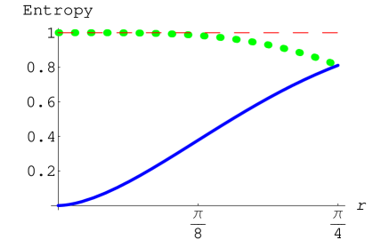
Figure 2: (Color online) Bipartite pure state entanglement. Thick solid curve (Blue): Anti-Rob in region II with (Alice and Rob in region I). Thin dashed curve (Red): Alice with (regions I and II). Dotted curve (Green): Rob in region I with (Alice and anti-Rob region II.)

V.2 Mixed state entanglement

For mixed state entanglement we can consider, besides the entanglement between the Minkowski mode $A$ and Rindler mode I calculated in Sec. IV, two additional bipartite divisions of the subsystems.

• The entanglement between mode $A$ and mode II. Tracing over the mode in region I, we obtain the density matrix

  $$\rho_{A,II}=\frac{1}{2}\left(\begin{array}[]{cccc}\cos^{2}r&0&0&0\\ 0&\sin^{2}r&\sin{r}&0\\ 0&\sin{r}&1&0\\ 0&0&0&0\end{array}\right).$$

  The partial transpose of $\rho_{A,II}$ is given by

  $$\rho^{T}_{A,II}=\frac{1}{2}\left(\begin{array}[]{cccc}\cos^{2}r&0&0&\sin{r}\\ 0&\sin^{2}r&0&0\\ 0&0&1&0\\ \sin{r}&0&0&0\end{array}\right),$$

  which has eigenvalues $(1,1,\sin^{2}r,-\sin^{2}r)/2$, the last of which $\lambda_{-}=-\frac{1}{2}\sin^{2}r$, is less than or equal to zero. At $r=0$ the eigenvalue is zero, which means that there is no entanglement at this point. However, for any $r>0$ entanglement does exist between these two modes according to the partial transpose criterion. The logarithmic negativity in this case is given by $N=\log_{2}(1+\sin^{2}r)$.

  Calculating the spin-flip of $\rho_{A,II}$

  $$\tilde{\rho}_{A,II}=\frac{1}{2}\left(\begin{array}[]{cccc}0&0&0&0\\ 0&1&\sin{r}&0\\ 0&\sin{r}&\sin^{2}{r}&0\\ 0&0&0&\cos^{2}{r}\end{array}\right),$$

  we find that

  $$\rho_{A,II}\,\tilde{\rho}_{A,II}=\frac{1}{2}\left(\begin{array}[]{cccc}0&0&0&0\\ 0&\sin^{2}{r}&\sin^{3}{r}&0\\ 0&\sin{r}&\sin^{2}{r}&0\\ 0&0&0&0\end{array}\right),$$

  has eigenvalues $(\sin^{2}r,0,0,0)$. Thus, the concurrence is given by $C(\rho_{A,II})=\lambda_{1}=\sin r$, which is zero at zero acceleration as expected, and approaches the value $1/\sqrt{2}$ for infinite acceleration $r\rightarrow\pi/4$. The entanglement of formation is

  $$E_{F}= - \frac{1}{2}(1+\cos{r})\log_{2}\left(\frac{1+\cos{r}}{2}\right)$$

  $$- \frac{1}{2}(1-\cos{r})\log_{2}\left(\frac{1-\cos{r}}{2}\right)$$

  and the mutual information is

  $$I = S(\rho_{A})+S(\rho_{II})-S(\rho_{A,II})$$

  $$= 1-\frac{1}{2}(1+\cos^{2}r)\log_{2}\left(\frac{1+\cos^{2}r}{2}\right)$$

  $$- \frac{1}{2}(1-\cos^{2}r)\log_{2}\left(\frac{1-\cos^{2}r}{2}\right)$$

  $$+ \frac{1}{2}\cos^{2}r\log_{2}\left(\frac{\cos^{2}r}{2}\right)$$

  $$+ (1-\frac{1}{2}\cos^{2}r)\log_{2}\left(1-\frac{1}{2}\cos^{2}r\right).$$

  At $r=0$ the mutual information is zero and approaches unity as the rate of acceleration goes to infinity.

• The entanglement between mode I and mode II. Tracing over the modes in $A$, we obtain the density matrix

  $$\rho_{I,II}=\frac{1}{2}\left(\begin{array}[]{cccc}\cos^{2}r&0&0&\cos{r}\sin{r}\\ 0&0&0&0\\ 0&0&1&0\\ \cos{r}\sin{r}&0&0&\sin^{2}r\end{array}\right).$$

  The partial transpose of $\rho_{I,II}$ (obtained by interchanging $I$’s qubits) is given by

  $$\rho^{T}_{I,II}=\frac{1}{2}\left(\begin{array}[]{cccc}\cos^{2}r&0&0&0\\ 0&0&\cos{r}\sin{r}&0\\ 0&\cos{r}\sin{r}&1&0\\ 0&0&0&\sin^{2}r\end{array}\right).$$

  which has eigenvalues $(2\sin^{2}r,2\cos^{2}r,1+(1+\sin^{2}2r)^{1/2},1-(1+\sin^{2}2r)^{1/2})/4$, the last of which $\lambda_{-}=-\frac{1}{4}[1-\sqrt{1+\sin^{2}2r}]$ is less than or equal to zero. Again, at $r=0$ there is no entanglement between these two subsystems. Yet, similar to the last case, entanglement does exist between these two modes in non-inertial frames according to the partial transpose criterion. Further, the logarithmic negativity $N=\log_{2}(\frac{1}{2}({1+\sqrt{1+\sin^{2}2r}}))$ is nonzero for all $r>0$. The spin-flip of $\rho_{I,II}$ is given by

  $$\tilde{\rho}_{I,II}=\frac{1}{2}\left(\begin{array}[]{cccc}\sin^{2}r&0&0&\cos r\sin{r}\\ 0&1&0&0\\ 0&0&0&0\\ \cos{r}\sin r&0&0&\cos^{2}r\end{array}\right),$$

  and the matrix

  $$\rho_{I,II}\,\tilde{\rho}_{I,II}=\frac{1}{2}\left(\begin{array}[]{cccc}\cos^{2}r\sin^{2}r&0&0&\cos^{3}r\sin{r}\\ 0&0&0&0\\ 0&0&0&0\\ \cos{r}\sin^{3}r&0&0&\cos^{2}r\sin^{2}r\end{array}\right),$$

  has eigenvalues $(\cos^{2}r\sin^{2}r,0,0,0)$.  Thus, the concurrence is given by $C(\rho_{I,II})=\lambda_{1}=\sin{r}\cos{r}$ which is zero at zero acceleration, and approaches the value $1/{2}$ for infinite acceleration $r\rightarrow\pi/4$. The entanglement of formation in this case is

  $$E_{F}= - \frac{(1+\sqrt{1-\sin^{2}{r}\cos^{2}{r}})}{2}\,\log_{2}\left(\frac{1+\sqrt{1-\sin^{2}{r}\cos^{2}{r}}}{2}\right)$$

  $$- \frac{(1-\sqrt{1-\sin^{2}{r}\cos^{2}{r}})}{2}\,\log_{2}\left(\frac{1-\sqrt{1-\sin^{2}{r}\cos^{2}{r}}}{2}\right),$$

  and the mutual information is

  $$I = S(\rho_{I})+S(\rho_{II})-S(\rho_{I,II})$$

  $$= -\frac{1}{2}\cos^{2}r\,\log_{2}\left(\frac{\cos^{2}r}{2}\right)$$

  $$- (1-\frac{1}{2}\cos^{2}r)\,\log_{2}\left(1-\frac{1}{2}\cos^{2}r\right)$$

  $$- \frac{1}{2}(1+\cos^{2}r)\,\log_{2}\left(\frac{1+\cos^{2}r}{2}\right)$$

  $$- \frac{1}{2}(1-\cos^{2}r)\,\log_{2}\left(\frac{1-\cos^{2}r}{2}\right)-1.$$

Again, we find that the mutual information is zero at $r=0$, and increases to a finite value (in this case $I=3/2\left(2-\log_{2}3\right)$), as the rate of acceleration goes to infinity. The results of the above calculations are shown in Figs. (3) - (5).

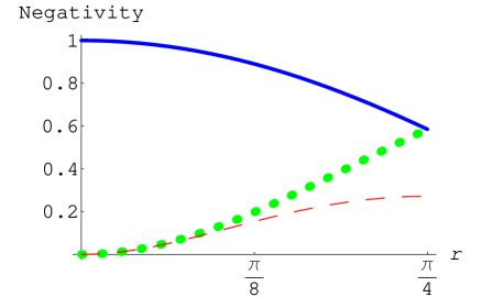
Figure 3: (Color online) The logarithmic negativity as a function of $r$. Thick solid curve (Blue): between Alice and Rob in region I. Thin dashed curve (Red): between the modes in regions I and II. Dotted curve (Green): between Alice and anti-Rob in region II.

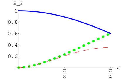
Figure 4: (Color online) Entanglement of formation as a function of $r$. Thick solid curve (Blue): between Alice and Rob in region I. Thin dashed curve (Red): between the modes in regions I and II. Dotted curve (Green): between Alice and anti-Rob in region II.

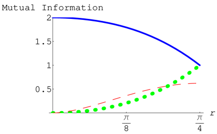
Figure 5: (Color online) Mutual information as a function of $r$. Thick solid curve (Blue): between Alice and Rob in region I. Thin dashed curve (Red): between the modes in regions I and II. Dotted curve (Green): between Alice and anti-Rob in region II.

V.3 Tripartite entanglement

Entanglement in triparite systems has been studied by Coffman, et. al., Coffman for the case of three qubits. They found that such quantum correlations cannot be arbitrarily distributed amongst the subsystems; the existence of three-body correlations constrains the distribution of the bipartite entanglement which remains after tracing over any one of the qubits. For example, in a GHZ-state, $|\mathrm{GHZ}\rangle=|000\rangle+|111\rangle$, tracing over one qubit results in maximally mixed state containing no entanglement between the remaining two qubits. In constrast, for a W-state, $|\mathrm{W}\rangle=|001\rangle+|010\rangle+|100\rangle$, the average remaining bipartite entanglement is maximal. Coffman, et. al., analyzed this phenomenon of entanglement sharing Coffman , using an entanglement monotone known as the tangle, defined as the square of the concurrence $\tau=C^{2}$ . They also introduced a new quantity, known as the residual tangle, in order to quantify the irreducible tripartite correlations in a system of three qubits ($a$, $b$, and $c$) Coffman . The definition is motivated by the observation that the tangle of $a$ with $b$ plus the tangle of $a$ with $c$ cannot exceed the tangle of $a$ with the joint subsystem $bc$, i.e.,

$$\tau_{a,b}+\tau_{a,c}\leq\tau_{a\left(b,c\right)}.$$ (43)

Subtracting the terms on the left hand side of Eq. (43) from that on the right hand side yields a nonnegative quantity referred to as the residual tangle $\tau_{a,b,c}$, i.e.,

$$\tau_{a,b,c}\equiv\tau_{a\left(b,c\right)}-\tau_{a,b}-\tau_{a,c}.$$ (44)

The residual tangle or ’three tangle’ is interpreted as quantifying the inherent tripartite entanglement present in a system of three qubits, i.e., the entanglement that cannot be accounted for in terms of the various bipartite tangles. This interpretation is given further support by the observation that the residual tangle is invariant under all possible permutations of the subsystem labels Coffman .

To quantify tripartite entanglement in our system we use the residual tangle $\tau_{A,I,II}=\tau_{A(I,II)}-\tau_{A,I}-\tau_{A,II}$. This quantity is zero for the situation we are considering, since $\tau_{A,I}=\cos^{2}r$, $\tau_{A,II}=\sin^{2}r$ and $\tau_{A(I,II)}=2(1-Tr[\rho_{I,II}^{2}])=1$. Thus, the state that we are studying has no tripartite correlations for any value of the acceleration rate. Instead, any entanglement existing in the system is necessarily bipartite in nature.

The marginal bipartite tangles, plotted in Fig. 6 as functions of $r$, are found to be strongly constrained. For low rates of acceleration, modes $A$ and I remain almost maximally entangled while there is very little entanglement between modes I and II and between modes $A$ and II. As the acceleration grows, the entanglement between modes I and II and between modes $A$ and II increases, while the entanglement between modes $A$ and I is degraded. The main system of interest (mode $A$ plus mode I) becomes increasingly entangled to mode II and therefore, after tracing over mode II, we observe an effect analogous to environmental decoherence in which the modes in region II play the role of the environment. The distribution of entanglement in the system is non-trivial since entanglement between modes $A$ and I is not conserved as it is in the inertial case.

VI Complementarity

We next analyze our system in terms of several complementarity relations designed to identify the different types of information encoded in a quantum state in an attempt to better understand how various subsystem properties depend on Rob’s rate of acceleration. Specifically, we are interested in explaining (i) the nonconservative nature of the entanglement discussed in the last section and (ii) the fact that not all of the initial entanglement between Alice and Rob is destroyed, even at infinite acceleration. The latter of these two results corresponds to the most obvious difference between the fermionic case studied here and the bosonic case investigated in ivette .

We begin by making use of the relationship Tessier

$$\eta\left(\rho\right)+\tau\left(\rho\right)+\overline{S^{2}}\left(\rho_{a}\right)+\overline{S^{2}}\left(\rho_{b}\right)=1,$$ (45)

which shows that an arbitrary state of two qubits ($a$ and $b$) exhibits a complementary tradeoff between the amounts of separable uncertainty $\eta$, bipartite entanglement (as quantified by the tangle) $\tau$, and a unitarily invariant measure of information about the single particle properties $\overline{S^{2}}$ that it encodes. The separable uncertainty

$$\eta\left(\rho\right)\equiv\mbox{\rm Tr}\left(\rho\tilde{\rho}\right)+M\left(\rho\right)-\tau\left(\rho\right),$$ (46)

$0\leq\eta\left(\rho\right)\leq 1,$ is a measure of the uncertainty or ignorance encoded in the two-qubit mixed state $\rho$ regarding individual subsystem properties that is unrelated to the presence of entanglement between the qubits. In Eq. (46), $\tilde{\rho}$ represents the spin-flip of $\rho$, and $M\left(\rho\right)\equiv 1-\mbox{\rm Tr}\left(\rho^{2}\right)$ is the marginal mixedness of $\rho$.

Similarly, $\overline{S^{2}}\left(\rho_{k}\right)$ is a measure of the information pertaining to a single qubit encoded in the marginal density operator $\rho_{k}$. Specifically, $\overline{S^{2}}\left(\rho_{k}\right)\equiv 1/2\left[\nu^{2}\left(\rho_{k}\right)+p^{2}\left(\rho_{k}\right)\right]$ is the average of the squares of the single qubit properties associated with qubit $k=a,b$. The first of these properties, the coherence $\nu$ of qubit $k$, quantifies, e.g., the fringe visibility in the context of a two-state system incident on an interferometer, and is given by

$$\nu\left(\rho_{k}\right)\equiv 2\left|\mbox{\rm Tr}\left(\rho_{k}\sigma_{+}^{\left(k\right)}\right)\right|,$$ (47)

where $\sigma_{+}^{\left(k\right)}=\left(\begin{array}[]{cc}0&1\\ 0&0\end{array}\right)$ is the raising operator acting on qubit $k$. Similarly, the predictability $p$ which quantifies the a priori information regarding whether qubit $k$ is in the state $\left|0\right\rangle$ or the state $\left|1\right\rangle$, e.g., whether it is more likely to take the upper or lower path in an interferometer, is given by

$$p\left(\rho_{k}\right)\equiv\left|\mbox{\rm Tr}\left(\rho_{k}\sigma_{z}^{\left(k\right)}\right)\right|,$$ (48)

where $\sigma_{z}=\left(\begin{array}[]{cc}1&0\\ 0&-1\end{array}\right)$ and $\left|0\right\rangle\left(\left|1\right\rangle\right)$ is the plus (minus) one eigenvector of $\sigma_{z}$.

Figures 6 and 7 plot the bipartite components of Eq. (45) for the various two-qubit marginals obtained after tracing over any one of the three subsystems ($A$, I, or II) as functions of the parameter $r$, while Fig. 8 does the same for the relevant single particle information measures. The complementary nature of these quantities is illustrated by the pattern/color scheme chosen for the curves, where each pattern (color) corresponds to a unique set of properties satisfying Eq. (45). Adding together all of the curves that contain a common attribute in Figs. 6 - 8 yields the constant value one, independent of $r$.

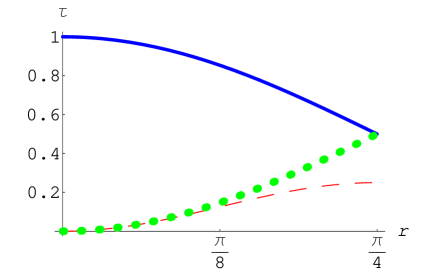
Figure 6: (Color online) Bipartite tangles as a function of $r$. Thick solid curve (Blue): between Alice and Rob in region I. Thin dashed curve (Red): between the modes in regions I and II. Dotted curve (Green): between Alice and anti-Rob in region II.

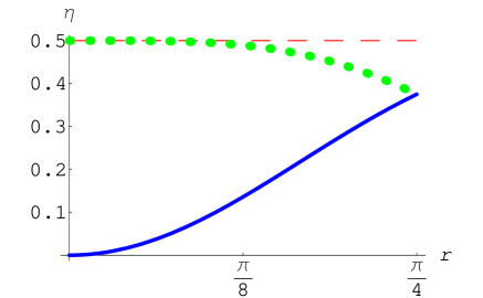
Figure 7: (Color online) Separable uncertainties as a function of $r$. Thick solid curve (Blue): between Alice and Rob in region I. Thin dashed curve (Red): between the modes in regions I and II. Dotted curve (Green): between Alice and anti-Rob in region II.

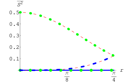
Figure 8: (Color online) Single qubit properties as a function of $r$. Dotted-solid line (Blue-Green): Alice (always zero). Thick-thin dashed curve (Blue-Red): Rob in region I. Dot-dashed curve (Green-Red): anti-Rob in region II.

For example, taking the sum of the two dashed (red) curves in Figs. 6 and 7 and the two curves containing dashes (red) in Fig. 8, thick-thin dashed (blue-red) and dot-dashed (green-red), corresponds to the equality $\tau_{I,II}+\eta_{I,II}+\overline{S^{2}}\left(\rho_{I}\right)+\overline{S^{2}}\left(\rho_{II}\right)=1$. Note that the curves in Fig. 8, representing information encoded in the individual qubits, each contribute to exactly two distinct complementarity relations.

The tradeoffs expressed by Eq. (45), and illustrated in Figs. 6 - 8, show how Rob’s acceleration determines the distribution of individual and bipartite properties of the system. For example, adding together the thick solid (blue) and dotted (green) curves in Fig. 6 shows that, although the entanglement in any bipartite subsystem changes with acceleration, the total entanglement between Alice and (the modes in regions I and II) is always maximal and constant. Further, since Rob is forced to trace over the causally disconnected modes in region II, the entanglement arising between the modes in region I and region II is ultimately responsible for the Unruh radiation that he sees. Indeed Alice, who has access to the modes in both regions, always sees an undisturbed vacuum. However, our analysis shows that the maximum amount of thermalization that Rob can experience (even at infinite acceleration) is limited by the amount of entanglement that exists between Alice and Rob in an inertial frame.

One straightforward way to see this is to consider the case in which Alice and Rob initially share no entanglement (e.g. an arbitrary product state between Alice and Rob). Then, as Rob’s acceleration approaches infinity, we find that $\tau_{I,II}$ approaches its maximum possible value of one (see Eq. (27) with $r=\pi/4$ note4 ). This is in contrast to the situation considered here in which the initial entanglement between Alice and Rob is maximal, constraining $\tau_{I,II}$ to a maximum value of 1/4.

Since the overall state of our system is always pure, we may also apply the result Peng

$$\tau_{a,b,c}+\tau^{\left(k\right)}+\overline{S^{2}}\left(\rho_{k}\right)=1,$$ (49)

which holds for an arbitrary pure state of three qubits ($a$, $b$, and $c$). The quantity $\tau^{\left(k\right)}\equiv\sum_{j\neq k}\tau_{j,k}$ is a measure of the total pairwise entanglement shared between qubit $k$ and all other qubits. Equation (49) quantifies an explicit tradeoff between the inherent three-body correlations in a tripartite system, the total pairwise entanglement of a selected qubit, and the single particle properties of the qubit.

Because the three tangle Eq. (44) is always zero for our system, this pure state complementarity relationship simplifies to

$$\tau^{\left(k\right)}+\overline{S^{2}}\left(\rho_{k}\right)=1.$$ (50)

It is then straightforward to see that this tradeoff is also captured by the pattern/color scheme used in the above figures. Simply adding the sum of any two curves in Fig. 6 to the curve in Fig. 8 that is composed of the same two attributes (or colors) again yields the constant value one, regardless of Rob’s acceleration. In particular, this shows that the entanglement between Alice and Rob in region I cannot vanish at infinite acceleration as it did in the bosonic case. This is because the entanglement $\tau_{I,II}$ generated between regions I and II (dashed/red curve in Fig. 6) and the single particle properties $\overline{S^{2}}\left(\rho_{I}\right)$ that manifest for Rob (dashed/red-blue curve in Fig. 8) are insufficient to satisfy Eq. (50). Instead, the contribution from the entanglement $\tau_{A,I}$ between Alice and Rob (solid/blue curve in Fig. 6) must also be taken into account to ensure that $\tau_{A,I}+\tau_{I,II}+\overline{S^{2}}\left(\rho_{I}\right)=1$.

Finally, we note that the various two-qubit marginal density operators for our system have a very specific form; they are all examples of the maximally entangled states with fixed marginal mixednesses (MEMMS) identified in Adesso . Indeed, this fact is closely related to the absence of tripartite correlations in our system, which implies that any entanglement that exists in the system must necessarily be bipartite. As shown in Tessier , the MEMMS are characterized by the relationship $M\left(\rho\right)=\eta\left(\rho\right)$, i.e., the marginal mixednesses are equal to the separable uncertainties. Thus, our fermionic system encodes the maximum amount of bipartite entanglement consistent with the separable uncertainty in each two-qubit marginal for every possible value of the acceleration rate.

VII Summary and Future Directions

We have studied the behavior of the entanglement between two modes of a free Dirac field in a non-inertial frame in flat spacetime from the point of view of two observers, Alice and Rob, in relative uniform acceleration. Our results show that entanglement existing between Alice and Rob in an inertial frame is progressively degraded by the Unruh effect as Rob’s rate of acceleration increases. However, unlike the bosonic case in which the inertial entanglement vanishes in the limit of infinite acceleration, in this case the entanglement achieves a minimum value of $1/\sqrt{2}$ for the entanglement of formation (and of $1/2$ for the tangle). This fundamental difference, a consequence of the fact that fermions have access to only two quantum levels vs. the infinite ladder of excitations available to bosons, means that in this case Alice and Rob always share some entanglement which can in principle be used as a resource for performing certain quantum information processing tasks. Further analysis shows that the total (quantum plus classical) correlations in the system, as quantified by the mutual information, behaves in a manner reminiscent of the bosonic case, decreasing from 2 for inertial observers to unity in the case of infinite acceleration.

Considering the (causally inaccessible to Rob) modes in region II to be a third subsystem allows us to analyze this system in terms of entanglement sharing. In doing so, we find that the overall tripartite pure state never encodes any inherently three-body correlations, regardless of the rate of acceleration. Any entanglement existing in the fermionic system is therefore necessarily bipartite. Such entanglement is known to be an invariant quantity for inertial observers, although different inertial observers may see these quantum correlations distributed among multiple degrees of freedom in different ways. However, in this analysis we find no indication that the entanglement in any bipartite subsystem is conserved when Rob is allowed to accelerate. In fact, our results show that the presence of the communication horizon, which isolates the modes in region II from an accelerated observer in region I, plays a key role in degrading the inertial entanglement between Alice and Rob.

Further insight into this behavior is gained by applying both pure and mixed state complementarity relations to different divisions of the system into subsystems. The ability of this formalism to identify the different types of information encoded in a quantum state facilitates the study of how various subsystem properties depend on Rob’s rate of acceleration. For instance, the constraints imposed by these relations illustrate how multi-qubit complementarity prevents the entanglement between Alice and Rob from vanishing at infinite acceleration as it does in the bosonic case. Additionally, we find that the amount of vacuum thermalization (due to Unruh radiation) that Rob experiences at infinite acceleration is constrained by the amount of entanglement that he shares with Alice in an inertial frame.

One possible avenue for further research along these lines is to study the entanglement between Alice and Rob in the case that Alice has acceleration $a_{1}$ and Rob has acceleration $a_{2}$. In this case the density matrix, after tracing over region II is

$$\rho_{A,I}=\frac{1}{2}\left(\begin{array}[]{cccc}\cos^{2}{r_{1}\cos^{2}{r_{2}}}&0&0&\cos{r_{1}}\cos{r_{2}}\\ 0&\cos^{2}{r_{1}}\sin^{2}{r_{2}}&0&0\\ 0&0&\sin^{2}{r_{1}}\cos^{2}{r_{2}}&0\\ \cos{r_{1}}\cos{r_{2}}&0&0&1+\sin^{2}{r_{1}}\sin^{2}{r_{2}}\end{array}\right)$$

where $\tan{r_{1}}=\exp(-\omega c/a_{1})$ and $\tan{r_{2}}=\exp\left(-\omega c/a_{2}\right)$. In this case the logarithmic negativity is $N=\log_{2}(1+\cos^{2}{r_{1}}\cos^{2}{r_{2}})$. Thus, we see that the entanglement is further degraded by having two accelerated observers, but again remains finite, in this case taking on the value $N=\log_{2}(5/4)$ in the infinite acceleration limit.

Another aspect of this problem that deserves further consideration is the nature of the communication that is and is not allowed between observers in different regions. Of course, no communication is possible between the left and right Rindler wedges (regions I and II). However, even when two parties are not causally disconnected from one another (e.g. Alice and Rob in Fig. 1), the presence of a horizon due to the acceleration of an observer imposes a unidirectionality on any classical communication occurring after the inertial observer crosses the horizon. Given the connection between the horizons seen by accelerated observers, and the event horizon of a black hole, this in turn suggests the potential for gaining further insight into questions related to the black hole information paradox.

- (1) The Physics of Quantum Information, Springer-Verlag 2000, D. Bouwmeester, A. Ekert, A. Zeilinger (Eds.).
- (2) Czachor, Phys. Rev. A 55, 72 (1997); D.R. Terno and A. Peres, Rev. Mod. Phys. 76, 93 (2004); A. Peres, P.F. Scudo and D.R. Terno, Phys. Rev. Lett. 88, 230402 (2002); Czachor, Phys. Rev. Lett. 94, 078901 (2005); P.M. Alsing and G.J. Milburn, Quant. Inf. Comp. 2, 487 (2002); R.M. Gingrich and C. Adami, Phys. Rev. Lett. 89, 270402 (2002); J. Pachos and E. Solano, QIC Vol. 3, No. 2, pp.115 (2003); W.T. Kim and E.J. Son, quant-ph/0408127; D. Ahn, H.J. Lee, Y.H. Moon, and S.W. Hwang, Phys. Rev. A 67, 012103 (2003). D. Ahn, H.J. Lee, and S.W. Hwang, e-print quant-ph:/0207018 (2002); D. Ahn, H.J. Lee, S.W. Hwang, and M.S. Kim, e-print quant-ph:/0207018 (2003). H. Terashima and M. Ueda, Int. J. Quant. Info. 1, 93 (2003). A.J. Bergou, R.M. Gingrich, and C. Adami, Phys. Rev. A 68, 042102 (2003). C. Soo and C.C.Y. Lin, Int. J. Quant. Info. 2, 183 (2003).
- (3) P.M. Alsing and G.J. Milburn, Phys. Rev. Lett. 91, 180404 (2003) and quant-ph/0302179; P.M. Alsing, D. McMahon and G.J. Milburn, J. Opt. B: Quantum Semiclass Opt. 6, S834 (2004).
- (4) I. Fuentes-Schuller and R.B. Mann, Phys.Rev.Lett. 95 (2005) 120404
- (5) J. Ball, I. Fuentes-Schuller and F.P. Schuller, quant-ph/0506113
- (6) V. Coffman, J. Kundu, and W. K. Wootters, Phys. Rev. A 61, 052306 (2000).
- (7) T. E. Tessier, Found. Phys. Lett. 18(2), 107 (2005).
- (8) W. K. Wootters, Phys. Rev. Lett. 80 2245 (1998).
- (9) G. Vidal and R. F. Werner Phys. Rev.A (65):032314, 2002; Plenio quant-ph/0505071, 2005.
- (10) R. S. Ingarden, A. Kossakowski and M. Ohya, Information Dynamics and Open Systems - Classical and Quantum Approach, (Kluwer Academic Publishers, Dordrecht, 1997). M.B.
- (11) F. Mandl and G. Shaw, Quantum Field Theory, Wiley, N.Y. (1984).
- (12) To cover the Minkowski regions III and IV in Fig. 1 one needs to switch in Eq. (III), which changes the Rindler metric in these regions to the form . This makes a spacelike coordinate and a timelike coordinate in region III and IV. We will not require the solutions to the Dirac equations in regions III and IV in order to discuss the entanglment between Alice and observers in region I and II.
- (13) In this work, we are implicitly assuming that the spin of each mode is along the direction of acceleration, the -axis. Since this motion is rectilinear, the succesive boosts into Rob’s instantaneous co-moving frame all commute. Hence, the spin does not suffer any Thomas precession (Wigner rotation) and therefore points along the same direction in both the inertial and non-inertial frames. See also rocio .
- (14) N.D. Birrel and P.C.W. Davies, Quantum fields in curved space, Cambridge Univ. Press, N.Y. (1982)
- (15) S.M. Carroll, Spacetime and Geometry, Addison and Wesley, p402-412 (2004).
- (16) In an arbitrary metric the Dirac inner product is given by where where is a spacelike hypersurface with normal and hyperspatial volume element , and is the adjoint of the Dirac spinor wave function . Here are the flat spacetime Dirac matrices satisfying with the Minkowski metric , while the matrices sastify the corresponding anti-commutation relations with the arbitrary metric, i.e. . The inner product is invariant under the choice of the spacelike hypersurface . For the choice corresponding to with in Minkowski coordinates, the inner product reduces to the usual flat spacetime form . In Rindler coordinates one can also choose to compute the inner product on the hypersurface , although it is often more convenient to perform the computation on the future horizon , ().
- (17) S. Takagi, Prog. Theor. Phys. Suppl. 88, 1-142 (1986).
- (18) R. Jáureguei, M. Torres and S. Hacyan, Phys. Rev. D 43, 3979 (1991).
- (19) D. McMahon, P.M. Alsing, P. Embid, The Dirac equation in Rindler space: a pedagogical introduction, gr-qc/0601010; W. Greiner, B. Müller and J. Rafelski, Quantum Electrodynamics of Strong Fields, Springer Verlag, N,Y., p563-571, (1985); M. Soffel, B. Müller and W. Greiner, Phys. Rev. D 22, 1935 (1980).
- (20) The Minkowski annihilation operator for frequency is related to the Rindler region I and region II operators of frequency more directly through an intermediate set of modes called Unruh modes unruh ; BD ; carroll . The Unruh modes analytically extend the Rindler region I modes to region II, and the region II modes to region I as discussed in the next paragraph. The Unruh modes are directly related to the Rindler region I and II modes through a Bogoliubov transformations of the form Eq. (14) and Eq. (21) takagi ; carroll . Since the Unruh modes exist over all Minkowski space, they share the same vacuum as the Minkowski annihilation operators. A Minkowski annihilation operator of frequency (a frequency which Alice detects) can be written as an integral (essentially a Fourier transform) over frequencies (that a Rindler observer detects) involving only Unruh annihilation operators with phase factor coefficients (seetakagi ). The single mode approximation entails assuming that Rob’s detector is sensitive to a single particle mode frequency (an extremely narrow band detector) and that the previously discussed frequency dependent phase factors are highly peaked about . We can then approximate the Minkowski annihilation operator by a single Unruh annihilation operator, which is then related to a Rindler particle annihilation operator in region I and a Rindler anti-particle creation operator in region II through a Bogoliubov transformation (see the discussion in the last paper in teleport ).
- (21) D.F. Walls and G.J. Milburn, Quantum Optics, Springer-Verlag, N.Y., (1994).
- (22) Similar relations exist for the operators and namely, , , , and . However, these operators correspond to the mode , which we have ignored in the single mode approximation.
- (23) P.C.W. Davies, J. of Phys. A8, 609 (1975); W.G. Unruh, Phys. Rev. D14, 870 (1976);
- (24) P.M. Alsing and P.W. Milonni, Am. J. Phys 72, 1524 (2004); quant-ph/0401170.
- (25) A. Peres , Phys. Rev. Lett. 77, 1413, (1996).
- (26) For a review on entanglement Dagmar Bruss J. Math. Phys., (43): 4237, 2002.
- (27) Let the intial unaccelerated state between Alice and Rob be the tensor product of Minkowski states where is any state (possibly mixed) for Alice and is any pure state for Rob. Since entanglement is invariant under local unitaries, we can always rotate to , the Minkowski vacuum for mode given in Eq. (27), without changing the initial entanglement. Then the reduced state for Rob is just , which has maximal entanglement between I and II at infinite acceleration.
- (28) X. Peng, X. Zhu, D. Suter, J. Du, M. Liu, and K. Gao, Phys. Rev. A 72, 052109/1 (2005).
- (29) G. Adesso, F. Illuminati, and S. De Siena, Phys. Rev. A 68, 062318-1 (2003).