Quantum Temporal Correlations and Entanglement via Adiabatic Control of Vector Solitons

Abstract

It is shown that optical pulses with an average position accuracy beyond the standard quantum limit can be produced by adiabatically expanding an optical vector soliton followed by classical dispersion management. The proposed scheme is also capable of entangling positions of optical pulses and can potentially be used for general continuous-variable quantum-information processing.

If an optical pulse consists of $N$ independent photons, then the uncertainty in the pulse-center position is the pulse width divided by $\sqrt{N}$, the so-called standard quantum limit giovannetti_science . The ultimate limit permissible by quantum mechanics, however, is determined by the Heisenberg uncertainty principle and is smaller than the standard quantum limit by another factor of $\sqrt{N}$, resulting in a quantum-enhanced accuracy useful for positioning and clock synchronization applications giovannetti_nature . To do better than the standard quantum limit, a multiphoton state with positive frequency correlations and, equivalently, negative time correlations is needed giovannetti_nature . Consequently, significant theoretical coincident ; tsang and experimental kuzucu efforts have been made to create such a nonclassical multiphoton state. All previous efforts were based on the phenomenon of spontaneous photon pair generation in parametric processes, limiting $N$ to 2 only. The resultant enhancement can only be regarded as a proof of concept and is too small to be useful, considering that a large number of uncorrelated photons can easily be obtained, with a standard quantum limit orders of magnitude lower than the ultimate limit achievable by two photons. It is hence much more desirable in practice to be able to enhance the position accuracy of a large number of photons. In this Letter, for the first time to the author’s knowledge, a scheme that produces a multiphoton state with positive frequency correlations among an arbitrary number of photons is proposed, thus enabling quantum position accuracy enhancement for macroscopic pulses as well. The scheme set forth therefore represents a major step forward towards the use of quantum enhancement in future positioning and clock synchronization applications.

The proposed scheme exploits the quantum properties of a vector soliton, in which photons in different optical modes are bound together by the combined effects of group-velocity dispersion, self-phase modulation, and cross-phase modulation agrawal . A quantum analysis shows that the average position of the photons in a vector soliton is insensitive to the optical nonlinearities and only subject to quantum dispersive spreading, while the separations among the photons is controlled by the balance between dispersion and nonlinearities. These properties are in fact very similar to those of scalar solitons lai ; kartner , so the idea of adiabatically compressing scalar solitons for momentum squeezing fini can be similarly applied to vector solitons. To produce negative time correlations, however, adiabatic soliton expansion should be performed instead. Given the past success of experiments on scalar quantum solitons soliton_experiments and vector solitons vs_experiments , the scheme set forth should be realizable with current technology. The formalism should apply to spatial vector solitons as well, so that the position accuracy of an optical beam can be enhanced barnett . Moreover, the proposed scheme is capable of creating temporal Einstein-Podolsky-Rosen (EPR) entanglement epr among the pulses in a vector soliton, suggesting that the vector soliton effect, together with quantum temporal imaging techniques tsang , may be used for general continuous-variable quantum-information processing braunstein .

For simplicity, only vector solitons with two optical modes, such as optical fiber solitons with two polarizations, are analyzed in this Letter, although the results can be naturally extended to multimode vector solitons, such as those studied in Refs. crosignani . Two-mode vector solitons are classically described by the coupled nonlinear Schrödinger equations agrawal , $i\frac{\partial U}{\partial t}=-b\frac{\partial^{2}U}{\partial z^{2}}+2c(|U|^{2}+B|V|^{2})U$ and $i\frac{\partial V}{\partial t}=-b\frac{\partial^{2}V}{\partial z^{2}}+2c(|V|^{2}+B|U|^{2})V$, where $U$ and $V$ are complex envelopes of the two polarizations, assumed to have identical group velocities and group-velocity dispersion, $t$ is the propagation time, $z$ is the longitudinal position coordinate in the moving frame of the pulses, $b$ is the group-velocity dispersion coefficient, $c$ is the self-phase modulation coefficient, and $Bc$ is the cross-phase modulation coefficient. For example, $B=2/3$ for linear polarizations in a linearly birefringent fiber menyuk , $B=2$ for circular polarizations in an isotropic fiber berkhoer , and $B=1$ describes Manakov solitons manakov , realizable in an elliptically birefringent fiber menyuk . $bc<0$ is required for solitons to exist. The coupled nonlinear Schrödinger equations can be quantized using the Hamiltonian $\hat{H}=\hbar\int dz\mbox{ }[b(\frac{\partial\hat{U}^{\dagger}}{\partial z}\frac{\partial\hat{U}}{\partial z}+\frac{\partial\hat{V}^{\dagger}}{\partial z}\frac{\partial\hat{V}}{\partial z})+c(\hat{U}^{\dagger}\hat{U}^{\dagger}\hat{U}\hat{U}+\hat{V}^{\dagger}\hat{V}^{\dagger}\hat{V}\hat{V}+2B\hat{U}^{\dagger}\hat{V}^{\dagger}\hat{U}\hat{V})]$, where $\hat{U}$ and $\hat{V}$ are photon annihilation operators of the two polarizations and the daggers denote the corresponding creation operators. The Heisenberg equations of motion derived from this Hamiltonian are analyzed using perturbative techniques by Rand et al. rand , who study the specific case of Manakov solitons, and by Lantz et al. lantz and Lee et al. lee , who numerically investigate the photon number entanglement in higher-order vector solitons. As opposed to these previous studies, in this Letter the exact quantum vector soliton solution is derived in the Schrödinger picture, in the spirit of the scalar soliton analyses in Refs. lai ; kartner .

Since the Hamiltonian conserves photon number in each mode and the average momentum, one can construct simultaneous Fock and momentum eigenstates with the Bethe ansatz $|n,m,p\rangle=\frac{1}{\sqrt{n!m!}}\int d^{n}x\mbox{ }d^{m}y\mbox{ }f_{nmp}(x_{1},...,x_{n},y_{1},...,y_{m})\times\hat{U}^{\dagger}(x_{1})...\hat{U}^{\dagger}(x_{n})\hat{V}^{\dagger}(y_{1})...\hat{V}^{\dagger}(y_{m})|0\rangle$ lai ; thacker , where $n$ and $m$ are the photon numbers in the two polarizations and $p$ is the average momentum. Using the Schrödinger equation $E|\Psi\rangle=\hat{H}|\Psi\rangle$, one obtains

$$E_{nmp}f_{nmp}(x_{1},...,x_{n},y_{1},...,y_{m}) =\hbar\bigg{\{}-b\sum_{j}\frac{\partial^{2}}{\partial x_{j}^{2}}-b\sum_{k}\frac{\partial^{2}}{\partial y_{k}^{2}}+2c\Big{[}\sum_{i<j}\delta(x_{j}-x_{i})+\sum_{l<k}\delta(y_{k}-y_{l})+B\sum_{j,k}\delta(x_{j}-y_{k})\Big{]}\bigg{\}}\times$$

$$\quad f_{nmp}(x_{1},...,x_{n},y_{1},...,y_{m}).$$ (1)

The soliton solution of Eq. (1) is

$$f_{nmp} =C_{nm}\exp\bigg{[}ip\Big{(}\sum_{j}x_{j}+\sum_{k}y_{k}\Big{)}+\frac{c}{2b}\Big{(}\sum_{i<j}|x_{j}-x_{i}|+\sum_{l<k}|y_{k}-y_{l}|+B\sum_{j,k}|x_{j}-y_{k}|\Big{)}\bigg{]},$$ (2)

where $C_{nm}$ is a normalization constant. The energy can be calculated by substituting Eq. (2) into Eq. (1) and is given by $E_{nmp}=\hbar bNp^{2}-\frac{\hbar c^{2}}{12b}[n(n^{2}-1)+m(m^{2}-1)+3B^{2}nm(n+m)]$, where $N=n+m$. A physical state should contain a distribution of momentum states, say, a Gaussian, such that the time-dependent multiphoton probability amplitude is now given by

$$f_{nm} =\int dp\mbox{ }\frac{1}{(2\pi\Delta p^{2})^{\frac{1}{4}}}\exp\Big{(}-\frac{p^{2}}{4\Delta p^{2}}-ibNp^{2}t\Big{)}f_{nmp}$$ (3)

$$=C_{nm}(8\pi)^{\frac{1}{4}}\Big{(}\frac{\Delta p}{1+4ibN\Delta p^{2}t}\Big{)}^{\frac{1}{2}}\exp\bigg{[}-\frac{\Delta p^{2}}{1+4ibN\Delta p^{2}t}\Big{(}\sum_{j}x_{j}+\sum_{k}y_{k}\Big{)}^{2}\bigg{]}\times$$ (4)

$$\quad\exp\bigg{[}\frac{c}{2b}\Big{(}\sum_{i<j}|x_{j}-x_{i}|+\sum_{l<k}|y_{k}-y_{l}|+B\sum_{j,k}|x_{j}-y_{k}|\Big{)}\bigg{]},$$ (5)

where $\Delta p$ is determined by initial conditions and a constant energy term that does not affect the position and momentum properties of a Fock state is omitted. Although a more realistic soliton state should have a superposition of Fock states resembling a coherent state lai , the Fock components of a coherent state for $N>>1$ have photon numbers very close to the mean value, so a Fock state should be able to adequately represent the position and momentum properties of a coherent-state soliton.

The multiphoton amplitude $f_{nm}$ consists of two components; a dispersive pulse-center component given by Eq. (4) that governs the quantum dispersion of the average photon position $\frac{1}{N}(\sum_{j}x_{j}+\sum_{k}y_{k})$, and a bound-state component given by Eq. (5) that fixes the distances among the photons via the attractive Kerr potentials. It follows that the momentum-space probability amplitude, defined as the $N$-dimensional Fourier transform of $f_{nm}$, also consists of an average momentum component and a bound-state component that governs the relative momenta among the photons.

If one increases $b$ or reduces $c$ adiabatically, the multiphoton amplitude would remain in the same form, but with increased uncertainties in the relative distances as well as reduced uncertainties in the relative momenta. More crucially, the average momentum uncertainty remains unaffected, leading to a multiphoton state with positive momentum correlations. The adiabatic approximation remains valid if the change happens over a propagation time scale $T>>\hbar/|E(t=T)-E(t=0)|$, which is on the order of the initial soliton period divided by $N$. As optical fiber solitons can typically propagate for a few soliton periods before loss becomes a factor, the desired adiabatic expansion should be realizable with current technology. In the following it is assumed for simplicity that only $c$ is adiabatically varied. Mathematically, in the limit of vanishing $c$, the bound-state component becomes relatively flat, and $f_{nm}$ becomes solely governed by the pulse-center component,

$$f_{nm}\propto\exp\bigg{[}-\frac{\Delta p^{2}}{1+4ibN\Delta p^{2}t}\Big{(}\sum_{j}x_{j}+\sum_{k}y_{k}\Big{)}^{2}\bigg{]}.$$ (6)

In the momentum space, as the bandwidth of the relative momenta is reduced and becomes much smaller than the bandwidth of the average momentum, the wavefunction in terms of momentum eigenstates becomes

$$|\Psi\rangle \propto\int dp\mbox{ }\exp\Big{(}-\frac{p^{2}}{4\Delta p^{2}}-ibNp^{2}t\Big{)}|n_{p},m_{p}\rangle,$$ (7)

where $|n_{p},m_{p}\rangle$ denotes a momentum eigenstate with momentum $p$ and $n$ and $m$ photons in the respective polarizations. Except for the dispersive phase term, Eq. (7) is precisely the desired coincident-frequency state that can achieve the ultimate limit of average position accuracy giovannetti_nature , as frequency is trivially related to momentum via the dispersion relation. If the pulse is sent across one channel only, adiabatic control of a scalar soliton would already suffice for the purpose of temporal uncertainty reduction, but the use of a vector soliton allows quantum-enhanced pulses to be sent across different channels, as originally envisioned by Giovannetti et al. giovannetti_nature , for additional security. The same operation of position squeezing on a scalar soliton is previously considered by Fini and Hagelstein, who nonetheless dismiss this possibility due to the detrimental effect of quantum dispersion fini .

Fortunately, quantum dispersion, like classical dispersion, can be compensated with classical dispersion management. If the vector soliton propagates in another linear waveguide with an opposite group-velocity dispersion $b^{\prime}$, such that $bt=-b^{\prime}t^{\prime}$, where $t$ is the propagation time in the first waveguide and $t^{\prime}$ is the propagation time in the second waveguide, then the dispersive phase term in Eq. (3), $-ibNp^{2}t$, can be cancelled, thus restoring the minimum uncertainty in the average photon position, while the pulse bandwidth remains constant because the second waveguide is linear. The complete proposed setup is sketched in Fig. 1. To apply the scheme set forth to a spatial vector soliton, negative refraction pendry is required to compensate for the quantum diffraction instead.

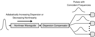
Figure 1: Proposed setup of generating multiphoton states with quantum-enhanced average position accuracy.

In order to understand how the quantum vector soliton solution corresponds to a classical soliton in typical experiments, consider the specific case of a Manakov soliton, where $B=1$. Other vector solitons should have very similar properties given the similarity of the solutions. If the photon position variables are re-indexed in the following new notations $\{z_{1},...,z_{N}\}=\{x_{1},...,x_{n},y_{1},...,y_{m}\}$, the multiphoton amplitude in Eqs. (4) and (5) becomes

$$f_{nm} =C_{nm}(8\pi)^{1/4}\Big{(}\frac{\Delta p}{1+4ibN\Delta p^{2}t}\Big{)}^{\frac{1}{2}}\times$$

$$\quad\exp\bigg{[}-\frac{\Delta p^{2}}{1+4ibN\Delta p^{2}t}\Big{(}\sum_{j}z_{j}\Big{)}^{2}+\frac{c}{2b}\sum_{i<j}|z_{j}-z_{i}|\bigg{]}.$$ (8)

Intriguingly, this solution is exactly the same as the scalar soliton solution lai , or in other words, a Manakov soliton is quantum-mechanically equivalent to a scalar soliton. This equivalence explains the discovery by Rand et al. that the squeezing effect of a Manakov soliton has the same optimum as a scalar soliton rand . Moreover, $C_{nm}$ can now be borrowed from the scalar soliton analysis and is given by $C_{nm}=[(N-1)!|c/b|^{N-1}/(2\pi)]^{1/2}$ lai . The knowledge of $C_{nm}$ allows one to calculate the correlations among the photon positions using standard statistical mechanics techniques. An expression for $\left\langle\sum_{i<j}|z_{j}-z_{i}|\right\rangle$ can be derived, and, by symmetry,

$$\left\langle|z_{j}-z_{i}|\right\rangle =\frac{1}{N(N-1)}\left\langle\sum_{i<j}|z_{j}-z_{i}|\right\rangle=\Big{|}\frac{2b}{Nc}\Big{|}\sim W_{0}.$$ (9)

As expected, the mean absolute distance between any two photons is on the order of the classical soliton pulse width, $W_{0}\sim|2b/(Nc)|$ lai . Next, assume that the variance of the relative distance is related to the square of the mean absolute distance by a parameter $q$,

$$\left\langle|z_{j}-z_{i}|^{2}\right\rangle =q\left\langle|z_{j}-z_{i}|\right\rangle^{2}=\frac{4qb^{2}}{N^{2}c^{2}}.$$ (10)

While an explicit expression for $q$ is hard to derive, $q$ must depend only on $N$ by dimensional analysis, must be larger than 1 because $\left\langle|z_{j}-z_{i}|^{2}\right\rangle\geq\left\langle|z_{j}-z_{i}|\right\rangle^{2}$, and is likely to be on the order of unity, as will be shown later. By symmetry, $\left\langle|z_{j}-z_{i}|^{2}\right\rangle=\left\langle z_{j}^{2}\right\rangle-2\left\langle z_{i}z_{j}\right\rangle+\left\langle z_{i}^{2}\right\rangle=2\left\langle z_{j}^{2}\right\rangle-2\left\langle z_{i}z_{j}\right\rangle$. Eq. (10) then gives

$$\left\langle z_{j}^{2}\right\rangle-\left\langle z_{i}z_{j}\right\rangle =\frac{2qb^{2}}{N^{2}c^{2}}.$$ (11)

Furthermore, the variance of $\sum_{j}z_{j}$ is simply given by

$$\left\langle\Big{(}\sum_{j}z_{j}\Big{)}^{2}\right\rangle =N\left\langle z_{j}^{2}\right\rangle+N(N-1)\left\langle z_{i}z_{j}\right\rangle=\Delta z^{2},$$ (12)

where $\Delta z^{2}=1/(4\Delta p^{2})+4(bN\Delta pt)^{2}$. From Eqs. (11) and (12) the covariances can be obtained explicitly,

$$\left\langle z_{j}^{2}\right\rangle =\frac{\Delta z^{2}}{N^{2}}+\frac{2q(N-1)b^{2}}{N^{3}c^{2}},\quad\left\langle z_{i}z_{j}\right\rangle=\frac{\Delta z^{2}}{N^{2}}-\frac{2qb^{2}}{N^{3}c^{2}}.$$ (13)

A quantum soliton solution best resembles a classical initial condition with independent photons when the initial covariance is zero, $\left\langle z_{i}z_{j}\right\rangle_{t=0}=1/(4N^{2}\Delta p^{2})-2qb^{2}/(N^{3}c^{2})|_{t=0}=0$, and

$$\Delta p =\Big{|}\frac{\sqrt{N}c}{\sqrt{8q}b}\Big{|}_{t=0}\sim\frac{1}{2\sqrt{N}W_{0}}.$$ (14)

Incidentally, the average momentum uncertainty $\Delta p$ is at the shot-noise level when the photons are initially uncorrelated. This justifies the assumption that $q$ is on the order of unity. An initial condition with independent photons would then mostly couple to a soliton state with $\Delta p$ given by Eq. (14), while coupling to continuum states should be negligible. Adiabatically increasing $|b/c|$ thus makes $\left\langle z_{i}z_{j}\right\rangle$ negative and therefore introduces the necessary negative correlations among the photon positions. To investigate the magnitude of the quantum enhancement in practice, it is useful to compare the quantum theory to the classical soliton theory, as the two regimes should converge when $N>>1$ and $\gamma<<\sqrt{N}$. According to the classical theory, if the ratio between the final and initial values of $|b/c|$ is $\gamma$, the pulse bandwidth is also reduced by a factor of $\gamma$, from $\sim 1/W_{0}$ to $\sim 1/(\gamma W_{0})$. Since the final average position uncertainty is the same as the input value, the accuracy enhancement over the standard quantum limit, for the same reduced bandwidth $\sim 1/(\gamma W_{0})$, is hence also given by $\gamma$, in the regime of moderate pulse expansion $\gamma<<\sqrt{N}$. Because the ultimate soliton state, given by Eqs. (6) and (7), has a bandwidth given by Eq. (14), $\sim 1/(\sqrt{N}W_{0})$, the ultimate limit is reached only when $\gamma>>\sqrt{N}$.

As the photons across different optical modes become correlated via the cross-phase modulation effect, entanglement is expected among the pulse positions in a vector soliton. To estimate the magnitude of the entanglement in terms of macroscopic position variables, consider again the case of Manakov solitons. Let the pulse-center coordinates of the respective polarizations be $X$ and $Y$, defined as $X=\frac{1}{n}\sum_{j=1}^{n}z_{j}$ and $Y=\frac{1}{m}\sum_{k=m+1}^{N}z_{k}$. If $n=m=N/2$ is assumed for simplicity, the following statistics for $X$ and $Y$ can be derived using Eqs. (13),

$$\left\langle\left(\frac{X+Y}{2}\right)^{2}\right\rangle =\frac{\Delta z^{2}}{N^{2}},\quad\left\langle\left(\frac{X-Y}{2}\right)^{2}\right\rangle=\frac{2qb^{2}}{N^{3}c^{2}}.$$ (15)

Similar to a two-photon vector soliton tsang , the average position of the two pulses is affected by quantum dispersion, while the relative distance is bounded by the Kerr effect. For two initially uncorrelated pulses, the two expressions in Eq. (15) have the same value. If, however, $b$ and $c$ are adiabatically manipulated, then the nonlocal uncertainty product $\left\langle(X-Y)^{2}\right\rangle\left\langle(P_{X}-P_{Y})^{2}\right\rangle$, where $P_{X}$ and $P_{Y}$ are the conjugate momenta, can remain constant under the adiabatic approximation, while $\left\langle(X-Y)^{2}\right\rangle$ and $\left\langle(P_{X}-P_{Y})^{2}\right\rangle$ can be arbitrarily varied. Since $\left\langle(P_{X}+P_{Y})^{2}\right\rangle$ always remains constant and $\left\langle(X+Y)^{2}\right\rangle$ can also remain the same as the input value if quantum dispersion is compensated, $\left\langle(X-Y)^{2}\right\rangle\left\langle(P_{X}+P_{Y})^{2}\right\rangle$ or $\left\langle(X+Y)^{2}\right\rangle\left\langle(P_{X}-P_{Y})^{2}\right\rangle$ can be arbitrarily reduced, thus resulting in EPR entanglement. Combined with quantum temporal imaging techniques, which are able to temporally reverse, compress, and expand photons in each mode tsang , adiabatic vector soliton control potentially provides a powerful way of fiber-based continuous-variable quantum-information processing braunstein .

Discussions with Demetri Psaltis and financial support by the Engineering Research Centers Program of the National Science Foundation under Award Number EEC-9402726 and the Defense Advanced Research Projects Agency (DARPA) are gratefully acknowledged.

I Erratum

On closer inspection, it is found that the soliton solution given by Eq. (2) and the expression for the energy $E_{mnp}$ below Eq. (2) in the published Letter tsang_prl are valid only for the Manakov soliton ($B=1$) or uncoupled scalar solitons ($B=0$). This can be seen by observing that the energies calculated using Eqs. (1) and (2) in Ref. tsang_prl in different regions of the configuration space are different unless $B=1$ or $B=0$. For example, for $n=2$ and $m=1$, the energy in the regions of $x_{1}<y_{1}<x_{2}$ and $x_{2}<y_{1}<x_{1}$ calculated using Eq. (2) is different from the energy in the other regions, unless $B=1$ or $B=0$.

This error does not affect the rest of Ref. tsang_prl that focuses on the Manakov soliton. Furthermore, it can be argued on physical grounds that the proposed scheme should still work for any positive $B$, despite the lack of an explicit soliton solution in general. First, it can be shown using the “center-of-mass” coordinate system hagelstein that all stable solutions of the Schrödginer equation given by Eq. (1) in Ref. tsang_prl must consist of a dispersive center-of-mass component and a bound-state component. For any positive $B$, the bound-state component must become flat in the ultimate limit of adiabatic pulse expansion, so any stable solution still approaches the form of Eqs. (6) and (7) in Ref. tsang_prl . Second, the average timing jitter of the two pulses is affected only by dispersion, regardless of $B$. If the net dispersion is zero and the fiber is assumed to be lossless, the output jitter is the same as the input jitter. As long as the solitary wave propagation is stable against the adiabatic change in fiber parameters, the bandwidth can be adiabatically reduced, leading to a raised timing standard quantum limit. Hence the final jitter must be lower than the raised standard quantum limit regardless of $B$. Finally, Eq. (1) in Ref. tsang_prl shows that the cross-phase modulation effect manifests itself as an attractive potential among photons across the two polarizations. In a stable solution of Eq. (1), the relative position and relative momentum of the two pulses can therefore be controlled by adjusting the balance between dispersion and cross-phase modulation. Since temporal entanglement has been proved to occur for the Manakov soliton in Ref. tsang_prl , this physical picture should remain qualitatively the same for a different cross-phase modulation coefficient, and temporal entanglement should also occur for any positive $B$.

There are also two typographical errors in tsang_prl . The factor $\frac{1}{N(N-1)}$ in Eq. (9) should read $\frac{2}{N(N-1)}$, and in the second-to-last paragraph, $Y=(1/m)\sum_{k=m+1}^{N}z_{k}$ should read $Y=(1/m)\sum_{k=n+1}^{N}z_{k}$. These typographical errors do not affect the rest of the Letter in any way.

References

- (1) V. Giovannetti, S. Lloyd, and L. Maccone, Science 306, 1330 (2004).
- (2) V. Giovannetti, S. Lloyd, and L. Maccone, Nature (London)412, 417 (2001).
- (3) V. Giovannetti et al., Phys. Rev. Lett. 88, 183602 (2002); Z. D. Walton et al., Phys. Rev. A67, 053810 (2003); J. P. Torres et al., Opt. Lett. 30, 314 (2005); M. Tsang and D. Psaltis, Phys. Rev. A71, 043806 (2005).
- (4) M. Tsang and D. Psaltis, Phys. Rev. A73, 013822 (2006).
- (5) O. Kuzucu et al., Phys. Rev. Lett. 94, 083601 (2005).
- (6) G. P. Agrawal, Nonlinear Fiber Optics (Academic Press, San Diego, 2001).
- (7) Y. Lai and H. A. Haus, Phys. Rev. A40, 844 (1989); ibid. 40, 854 (1989).
- (8) F. X. Kärtner and H. A. Haus, Phys. Rev. A48, 2361 (1993); P. L. Hagelstein, ibid. 54, 2426 (1996).
- (9) J. M. Fini and P. L. Hagelstein, Phys. Rev. A66, 033818 (2002).
- (10) See, for example, A. Sizmann, Appl. Phys. B 65, 745 (1997), and references therein; Ch. Silberhorn et al., Phys. Rev. Lett. 86, 4267 (2001).
- (11) See, for example, M. N. Islam, Opt. Lett. 14, 1257 (1989); J. U. Kang et al., Phys. Rev. Lett. 76, 3699 (1996); Y. Barad and Y. Silberberg, ibid. 78, 3290 (1997); S. T. Cundiff et al., ibid. 82, 3988 (1999).
- (12) S. M. Barnett, C. Fabre, and A. Mâitre, Eur. Phys. J. D 22, 513 (2003).
- (13) A. Einstein, B. Podolsky, and N. Rosen, Phys. Rev. 47, 777 (1935).
- (14) S. L. Braunstein and P. van Loock, Rev. Mod. Phys. 77, 513 (2005).
- (15) B. Crosignani and P. Di Porto, Opt. Lett. 6, 329 (1981); F. T. Hioe, Phys. Rev. Lett. 82, 1152 (1999).
- (16) C. R. Menyuk, IEEE J. Quantum Electron. 25, 2674 (1989).
- (17) A. L. Berkhoer and V. E. Zakharov, Sov. Phys. JETP 31, 486 (1970).
- (18) S. V. Manakov, Sov. Phys. JETP 38, 248 (1974).
- (19) D. Rand, K. Steiglitz, and P. R. Prucnal, Phys. Rev. A71, 053805 (2005).
- (20) E. Lantz et al., J. Opt. B 6, S295 (2004).
- (21) R.-K. Lee, Y. Lai, and B. A. Malomed, Phys. Rev. A71, 013816 (2005).
- (22) H. B. Thacker, Rev. Mod. Phys. 53, 253 (1981).
- (23) V. G. Veselago, Sov. Phys. Usp. 10, 509 (1968); J. B. Pendry, Phys. Rev. Lett. 85, 3966 (2000).

References

- (1) M. Tsang, Phys. Rev. Lett. 97, 23902 (2006).
- (2) P. L. Hagelstein, Phys. Rev. A54, 2426 (1996).