Propagation of temporal entanglement

Abstract

The equations that govern the temporal evolution of two photons in the Schrödinger picture are derived, taking into account the effects of loss, group-velocity dispersion, temporal phase modulation, linear coupling among different optical modes, and four-wave mixing. Inspired by the formalism, we propose the concept of quantum temporal imaging, which uses dispersive elements and temporal phase modulators to manipulate the temporal correlation of two entangled photons. We also present the exact solution of a two-photon vector soliton, in order to demonstrate the ease of use and intuitiveness of the proposed formulation.

I Introduction

In quantum optics, the Heisenberg picture, where optical fields are treated as conjugate positions and momenta of quantized harmonic oscillators, is often preferred, as it is easy to substitute the optical fields in classical electromagnetic problems with non-commutative operators and obtain the Heisenberg equations of motion. Once the operator equations are solved, one can then obtain various quantum properties of the optical fields via non-commutative algebra. However, the Heisenberg picture is not without shortcomings. It can be hard to analytically or numerically solve the complex or nonlinear operator equations without approximations. It is also difficult to grasp any intuition about how the quantum correlations among the photons evolve until the Heisenberg equations are solved. These difficulties have led to a growing appreciation of the Schrödinger picture, where the photons are treated as an ensemble of bosons, and the evolution of the many-photon probability amplitude is studied. This arguably more intuitive approach has led to great success in the quantum theory of solitons lai , where instead of solving the formidable nonlinear operator equations, one can obtain analytic solutions from the linear boson equations in the Schrödinger picture. The many-boson interpretation has been applied to the study of entangled photons as well, where the two-photon probability amplitude is shown to obey the Wolf equations by Saleh, Teich, and Sergienko (STS) saleh . Instead of treating the entanglement properties of the photons and the optical propagation as two separate problems, with the STS equations, one can now use a single quantity, namely the two-photon amplitude, to keep track of the spatiotemporal entanglement evolution in free space. This is analogous to the Wolf equations, which reformulate the laws of optics in terms of coherence propagation wolf .

In this paper, we utilize the STS treatment of two photons to study various temporal effects, in the hope that the Schrödinger picture would offer a more accessible interpretation of temporal entanglement propagation for analytic or numerical studies of two-photon systems. Loss, group-velocity dispersion, temporal phase modulation, via an electro-optic modulator for example, linear mode coupling, via a beam splitter or a fiber coupler for example, and four-wave mixing, in a coherently prepared atomic gas lukin for example, are all included in our proposed formalism, thus extending the STS model for use in many more topics in quantum optics, such as nonlocal dispersion cancellation franson ; steinberg , fourth-order interferometry hom , and two-photon nonlinear optics lukin ; chiao . The analysis of a two-photon vector soliton, consisting of two photons in orthogonal polarizations under the cross-phase modulation effect, is presented in the final section, in order to demonstrate the ease of use and intuitiveness of the Schrödinger picture.

Inspired by the formalism set forth, we propose the concept of quantum temporal imaging, which uses dispersive elements and temporal phase modulators to manipulate the temporal entanglement properties of two photons. Most significantly, we show that it is possible to convert positive time correlation to negative time correlation, or vice versa, using a temporal imaging system. This conversion technique should be immensely useful for applications that require negative time correlation, such as quantum-enhanced clock synchronization giovannetti_nature . Although there have been theoretical giovannetti ; walton ; torresOL ; tsangPRA and experimental kuzucu proposals of generating negative time correlation directly, they have various shortcomings compared with the conventional tried-and-true schemes that generate positive time correlation. Our proposed technique should therefore allow more flexibility in choosing two-photon sources for quantum optics applications.

The paper is structured as follows: Sec. II derives the equations that describe the evolution of the two-photon amplitude in two separate modes, Sec. III introduces the principles of quantum temporal imaging, Sec. IV includes linear mode coupling in the formalism, Sec. V generalizes the formalism to two photons in more than two modes, Sec. VI includes the effect of four-wave mixing, and Sec. VII presents the exact solution of a two-photon vector soliton.

II Two Photons in Two Separate Modes

Let us first consider two photons in two optical modes, such as two polarizations, two propagation directions or two waveguide modes. The corresponding two-photon wavefunction is

$$|\Psi\rangle =C_{12}|1,1\rangle+C_{11}|2,0\rangle+C_{22}|0,2\rangle,$$ (1)

where the constants $C_{jk}$’s are the overall amplitudes of the quantum states, $|1,1\rangle$ is the quantum state in which one photon is in each mode, $|2,0\rangle$ is the state in which both photons are in mode 1, and $|0,2\rangle$ is the state which both photons are in mode 2. The positive-frequency forward-propagating component of the electric field in each mode is given by huttner ; matloob

$$\hat{E}^{(+)}_{j}(z,t) =i\int_{0}^{\infty}d\omega\mbox{ }\Big{(}\frac{\hbar\omega\eta_{j}(\omega)}{4\pi\epsilon_{0}c[n_{j}(\omega)]^{2}S}\Big{)}^{\frac{1}{2}}\times$$

$$\quad\hat{a}_{j}(z,\omega)\exp(-i\omega t),$$ (2)

where $n_{j}$ is the complex, frequency-dependent refractive index in mode $j$, $\eta_{j}$ is the real part of $n_{j}$, $S$ is an area of quantization in the $x$-$y$ plane, and $\hat{a}_{j}$ is the photon annihilation operator, related to the corresponding creation operator via the equal-space commutator huttner ; matloob ,

$$[\hat{a}_{j}(z,\omega),\hat{a}_{j}^{\dagger}(z,\omega^{\prime})] =\delta(\omega-\omega^{\prime}),\quad j=1,2.$$ (3)

In the Heisenberg picture, the creation and annihilation operators evolve according to the following equations huttner ; matloob ,

$$\frac{\partial\hat{a}_{1}(z,\omega)}{\partial z} =i\frac{\omega n_{1}(\omega)}{c}\hat{a}_{1}(z,\omega)+$$

$$\quad i\Big{(}\frac{2\omega\mu_{1}(\omega)}{c}\Big{)}^{\frac{1}{2}}\hat{f}_{1}(z,\omega),$$ (4)

$$\frac{\partial\hat{a}_{2}(z^{\prime},\omega^{\prime})}{\partial z^{\prime}} =i\frac{\omega^{\prime}n_{2}(\omega^{\prime})}{c}\hat{a}_{2}(z^{\prime},\omega^{\prime})+$$

$$\quad i\Big{(}\frac{2\omega^{\prime}\mu_{2}(\omega^{\prime})}{c}\Big{)}^{\frac{1}{2}}\hat{f}_{2}(z^{\prime},\omega^{\prime}),$$ (5)

where $\mu_{j}$ is the imaginary part of $n_{j}$, and $\hat{f}_{j}$ is the Langevin noise operator, satisfying the commutation relation,

$$[\hat{f}_{j}(z,\omega),\hat{f}_{j}^{\dagger}(z^{\prime},\omega^{\prime})] =\delta(z-z^{\prime})\delta(\omega-\omega^{\prime}).$$ (6)

To proceed, we replace $\omega n_{j}(\omega)/c$ by the following phenomenological approximation agrawal ,

$$\frac{\omega n_{j}(\omega)}{c} \approx i\frac{\alpha_{j}}{2}+\sum_{n=0}^{2}\frac{\beta_{nj}}{n!}(\omega-\omega_{0})^{n}+\frac{\omega_{0}}{c}\Delta n_{j},$$ (7)

where $\alpha_{j}=2Im[k_{j}(\omega_{0})]$ is the loss coefficient, $\beta_{nj}=\partial^{n}Re[k_{j}(\omega)]/\partial\omega^{n}|_{\omega=\omega_{0}}$ is the $n$th-order dispersion coefficient, and $\Delta n_{j}$ encompasses any other refractive index perturbation. Defining the slowly-varying envelope operators as

$$\hat{A}_{j}(z,t) =\exp(-i\beta_{0j}z+i\omega_{0}t)\int_{0}^{\infty}\frac{d\omega}{\sqrt{2\pi}}\mbox{ }\hat{a}_{j}(z,\omega)\exp(-i\omega t),$$ (8)

where $\omega_{0}$ is the carrier frequency of the two modes, one can obtain two evolution equations for the envelope operators,

$$\frac{\partial}{\partial z}\hat{A}_{1}(z,t) =iK_{1}\Big{(}t,i\frac{\partial}{\partial t}\Big{)}\hat{A}_{1}(z,t)+\hat{F}_{1},$$ (9)

$$\frac{\partial}{\partial z^{\prime}}\hat{A}_{2}(z^{\prime},t^{\prime}) =iK_{2}\Big{(}t^{\prime},i\frac{\partial}{\partial t^{\prime}}\Big{)}\hat{A}_{2}(z^{\prime},t^{\prime})+\hat{F}_{2},$$ (10)

$$K_{j}\Big{(}t,i\frac{\partial}{\partial t}\Big{)} =\Big{[}\frac{i\alpha_{j}}{2}+i\beta_{1j}\frac{\partial}{\partial t}-\frac{\beta_{2j}}{2}\frac{\partial^{2}}{\partial t^{2}}+\frac{\omega_{0}}{c}\Delta n_{j}(t)\Big{]},$$ (11)

where $\hat{F}_{j}$ is defined as,

$$\hat{F}_{j}(z,t) =\exp(-i\beta_{0j}z+i\omega_{0}t)\times$$

$$\quad\int_{0}^{\infty}\frac{d\omega}{\sqrt{2\pi}}\mbox{ }i\Big{(}\frac{2\omega\mu_{j}(\omega)}{c}\Big{)}^{\frac{1}{2}}\hat{f}_{j}(z,\omega)\exp(-i\omega t),$$ (12)

and $K_{j}$ is the complex wavenumber for the slowly-varying envelope. $\Delta n_{j}$ can explicity depend on time, if the perturbation is much slower than the optical-frequency oscillation so that an adiabatic approximation can be made, such as in an electro-optic modulator.

We now define the two-photon probability amplitudes as

$$\psi_{12}(z,t,z^{\prime},t^{\prime}) =\langle 0|\hat{A}_{1}(z,t)\hat{A}_{2}(z^{\prime},t^{\prime})|\Psi\rangle,$$ (13)

$$\psi_{11}(z,t,z^{\prime},t^{\prime}) =\frac{1}{\sqrt{2}}\langle 0|\hat{A}_{1}(z,t)\hat{A}_{1}(z^{\prime},t^{\prime})|\Psi\rangle,$$ (14)

$$\psi_{22}(z,t,z^{\prime},t^{\prime}) =\frac{1}{\sqrt{2}}\langle 0|\hat{A}_{2}(z,t)\hat{A}_{2}(z^{\prime},t^{\prime})|\Psi\rangle.$$ (15)

The physical significance of each amplitude $\psi_{jk}$ is that its magnitude squared gives the probability density, $P_{jk}$, of coincidentally measuring one photon in mode $j$ at $(z,t)$ and another photon in mode $k$ at $(z^{\prime},t^{\prime})$,

$$P_{jk}(z,t,z^{\prime},t^{\prime}) =|\psi_{jk}(z,t,z^{\prime},t^{\prime})|^{2}.$$ (16)

Temporal entanglement is defined as the irreducibility of $|\psi_{12}|^{2}$ into a product of one-photon amplitudes in the form of $a(t)b(t^{\prime})$. This means that the probability of detecting a photon in mode $1$ at time $t$ is correlated to the probability of detecting a photon in mode $2$ at $t^{\prime}$. The most popular ways of generating entangled photons are spontaneous parametric down conversion klyshko and four-wave mixing fiorentino , where the wave mixing geometry and the spatiotemporal profile of the pump beam determine the initial $\psi_{12}$.

To obtain the evolution equations for the two-photon amplitude $\psi_{12}(z,t,z^{\prime},t^{\prime})$ in the Schrödinger picture, we employ the same trick as in Ref. saleh . First we multiply Eq. (9) with $\hat{A}_{2}(z^{\prime},t^{\prime})$ and Eq. (10) with $\hat{A}_{1}(z,t)$ to produce two equations,

$$\frac{\partial}{\partial z}\hat{A}_{1}(z,t)\hat{A}_{2}(z^{\prime},t^{\prime}) =iK_{1}\Big{(}t,i\frac{\partial}{\partial t}\Big{)}\hat{A}_{1}(z,t)\hat{A}_{2}(z^{\prime},t^{\prime})+\hat{F}_{1}\hat{A}_{2},$$ (17)

$$\frac{\partial}{\partial z^{\prime}}\hat{A}_{1}(z,t)\hat{A}_{2}(z^{\prime},t^{\prime}) =iK_{2}\Big{(}t^{\prime},i\frac{\partial}{\partial t^{\prime}}\Big{)}\hat{A}_{1}(z,t)\hat{A}_{2}(z^{\prime},t^{\prime})+\hat{F}_{2}\hat{A}_{1}.$$ (18)

Using the definition of $\psi_{12}$ in Eq. (13) and assuming that the thermal reservoirs are in the vacuum state so that the Langevin operators evaluate to zero when applied to the wavefunction jeffers , a pair of equations in terms of $\psi_{12}$ are derived,

$$\frac{\partial}{\partial z}\psi_{12}(z,t,z^{\prime},t^{\prime}) =iK_{1}\Big{(}t,i\frac{\partial}{\partial t}\Big{)}\psi_{12}(z,t,z^{\prime},t^{\prime}),$$ (19)

$$\frac{\partial}{\partial z^{\prime}}\psi_{12}(z,t,z^{\prime},t^{\prime}) =iK_{2}\Big{(}t^{\prime},i\frac{\partial}{\partial t^{\prime}}\Big{)}\psi_{12}(z,t,z^{\prime},t^{\prime}).$$ (20)

Equations (19) and (20) are the temporal version of the STS equations saleh , including the effects of loss, dispersion and phase modulation. They can also be written in the frequency domain as

$$\phi_{12}(z,\Omega,z^{\prime},\Omega^{\prime}) =\int_{-\infty}^{\infty}dt\int_{-\infty}^{\infty}dt^{\prime}\mbox{ }\psi_{12}(z,t,z^{\prime},t^{\prime})\times$$

$$\quad\exp(i\Omega t+i\Omega^{\prime}t^{\prime}),$$ (21)

$$\frac{\partial}{\partial z}\phi_{12}(z,\Omega,z^{\prime},\Omega^{\prime}) =iK_{1}\Big{(}\frac{1}{i}\frac{\partial}{\partial\Omega},\Omega\Big{)}\phi_{12}(z,\Omega,z^{\prime},\Omega^{\prime}),$$ (22)

$$\frac{\partial}{\partial z^{\prime}}\phi_{12}(z,\Omega,z^{\prime},\Omega^{\prime}) =iK_{2}\Big{(}\frac{1}{i}\frac{\partial}{\partial\Omega^{\prime}},\Omega^{\prime}\Big{)}\phi_{12}(z,\Omega,z^{\prime},\Omega^{\prime}).$$ (23)

For entangled photons, because $\psi_{12}$ or $\phi_{12}$ cannot be separated into a product of one-photon amplitudes, distortions experienced in one arm can coherently add to the distortions experienced in the other arm, leading to various nonlocal quantum effects.

For example, consider group-velocity dispersion only, the output $\phi_{12}$ is given by

$$\quad\phi_{12}(z,\Omega,z^{\prime},\Omega^{\prime})$$

$$=\exp\Big{(}i\beta_{11}\Omega z+i\beta_{12}\Omega^{\prime}z^{\prime}+\frac{i\beta_{21}}{2}\Omega^{2}z+\frac{i\beta_{22}}{2}\Omega^{\prime 2}z^{\prime}\Big{)}\times$$

$$\quad\phi_{12}(0,\Omega,0,\Omega^{\prime}).$$ (24)

If the photons are initially entangled with negative frequency correlation, $\phi_{12}(0,\Omega,0,\Omega^{\prime})$ can be approximated by $\phi(\Omega)\delta(\Omega+\Omega^{\prime})$. Ignoring the unimportant linear spectral phase, the output is

$$\phi_{12}(z,\Omega,z^{\prime},\Omega^{\prime}) =\exp\Big{[}\frac{i\Omega^{2}}{2}(\beta_{21}z+\beta_{22}z^{\prime})\Big{]}\phi(\Omega)\delta(\Omega+\Omega^{\prime}).$$ (25)

Hence if $\beta_{21}z=-\beta_{22}z^{\prime}$, the dispersion effects in both arms can nonlocally cancel each other, as originally discovered by Franson franson .

III Quantum Temporal Imaging

In the Schrödinger picture, the two-photon amplitude evolves under temporal effects. Since the entanglement properties of the photons are contained in the two-photon amplitude, the Schrödinger picture allows one to use the temporal effects to engineer the entanglement.

First, consider the evolution of the two-photon amplitude when one of the modes, say mode 1, is subject to group-velocity dispersion,

$$\frac{\partial\psi_{12}}{\partial z} =-\beta_{11}\frac{\partial\psi_{12}}{\partial t}-\frac{i\beta_{21}}{2}\frac{\partial^{2}\psi_{12}}{\partial t^{2}},$$ (26)

$$\psi_{12}(L,t,z^{\prime},t^{\prime}) =\int_{-\infty}^{\infty}d\tau\mbox{ }b_{1}(t-\tau)\psi_{12}(0,\tau,z^{\prime},t^{\prime}),$$ (27)

$$b_{1}(t-\tau) =\Big{(}\frac{i}{2\pi\beta_{21}L}\Big{)}^{\frac{1}{2}}\exp\Big{[}\frac{-i(t-\beta_{11}L-\tau)^{2}}{2\beta_{21}L}\Big{]}.$$ (28)

Group-velocity dispersion is well known to be analogous to Fresnel diffraction.

Next, consider a quadratic temporal modulation of refractive index imposed on mode 1 by a short or traveling-wave electro-optic modulator,

$$\frac{\partial\psi_{12}}{\partial z} =\frac{ik_{0}\Delta n_{2}(t-t_{0})^{2}}{2}\psi_{12},$$ (29)

$$\psi_{12}(l,t,z^{\prime},t^{\prime}) =q(t)\psi_{12}(0,t,z^{\prime},t^{\prime}),$$ (30)

$$q(t) =\exp\Big{[}\frac{ik_{0}\Delta n_{2}l}{2}(t-t_{0})^{2}\Big{]}.$$ (31)

Quadratic temporal phase modulation is analogous to a lens. $\Delta n_{2}$ is assumed to be a constant, and $t_{0}$ is the time delay of the modulation. Kerr effect by a co-propagating classical pulse would also suffice.

Two dispersive elements and a quadratic phase modulator in-between form a temporal imaging system, which has been well studied in the classical domain kolner . Suppose that the photon in mode 1 propagates through the first dispersive element, with an effective dispersion coefficient $\beta_{21}$ and effective length $L$, then passes through a time lens with refractive index modulation $\Delta n_{2}(t-t_{0})^{2}/2$, and finally propagates through the second dispersive element, with an effective dispersion coefficient $\beta_{21}^{\prime}$ and effective length $L^{\prime}$. The output two-photon amplitude can be expressed in terms of the input as

$$\psi_{12}(z,t,z^{\prime},t^{\prime}) =\int_{-\infty}^{\infty}d\tau\int_{-\infty}^{\infty}d\tau^{\prime}\mbox{ }b_{1}^{\prime}(t-\tau^{\prime})q(\tau^{\prime})b_{1}(\tau^{\prime}-\tau)\times$$

$$\quad\psi_{12}(0,\tau,z^{\prime},t^{\prime}),$$ (32)

$$b_{1}^{\prime}(t-\tau^{\prime}) =\Big{(}\frac{i}{2\pi\beta_{21}^{\prime}L^{\prime}}\Big{)}^{\frac{1}{2}}\exp\Big{[}\frac{-i(t-\beta_{11}^{\prime}L^{\prime}-\tau^{\prime})^{2}}{2\beta_{21}^{\prime}L^{\prime}}\Big{]}.$$ (33)

When the “lens law” for the time domain is satisfied,

$$\frac{1}{\beta_{21}L}+\frac{1}{\beta_{21}^{\prime}L^{\prime}} =k_{0}\Delta n_{2}l,$$ (34)

the impulse response of the system becomes

$$h(t,\tau) =\int_{-\infty}^{\infty}d\tau^{\prime}\mbox{ }b_{1}^{\prime}(t-\tau^{\prime})q(\tau^{\prime})b_{1}(\tau^{\prime}-\tau)$$ (35)

$$=\frac{i}{2\pi\sqrt{\beta_{21}L\beta_{21}^{\prime}L^{\prime}}}\exp\Big{[}\frac{-i(t-\beta_{11}^{\prime}L^{\prime})^{2}}{2\beta_{21}^{\prime}L^{\prime}}\Big{]}\times$$

$$\quad\exp\Big{[}\frac{-i(\tau+\beta_{11}L)^{2}}{2\beta_{21}L}\Big{]}\int_{-\infty}^{\infty}d\tau^{\prime}\mbox{ }P(\frac{\tau^{\prime}}{T_{a}})\times$$

$$\quad\exp\Big{[}i\Big{(}\frac{t-\beta_{11}^{\prime}L^{\prime}}{\beta_{21}^{\prime}L^{\prime}}+\frac{\tau+\beta_{11}L}{\beta_{21}L}-k_{0}\Delta n_{2}lt_{0}\Big{)}\tau^{\prime}\Big{]},$$ (36)

where $P(\tau^{\prime}/T_{a})$ is the normalized temporal aperture function of the time lens that can be used to describe any deviation of the actual temporal phase modulation from the ideal quadratic profile, such as truncation or higher-order phase modulation, and $T_{a}$ is the aperture width. If

$$T_{a}>>\frac{\beta_{2}L}{T_{0}},$$ (37)

where $T_{0}$ is the smallest feature size of $\psi_{12}$ along the $t$ axis, the integral in Eq. (36) can be approximated by a delta function. We then arrive at the input-output relation for the two-photon amplitude,

$$\psi_{12}(z,t,z^{\prime},t^{\prime}) =\frac{1}{\sqrt{M}}\psi_{12}(0,\frac{t-t_{d}}{M},z^{\prime},t^{\prime}),$$ (38)

$$t_{d} =\beta_{11}^{\prime}L^{\prime}+M\beta_{11}L+(1-M)t_{0},$$ (39)

$$M =-\frac{\beta_{21}^{\prime}L^{\prime}}{\beta_{21}L},$$ (40)

where an unimportant quadratic phase factor is omitted, $t_{d}$ is the time delay of the system, and $M$ is the magnification, which can be positive or negative depending on the signs of $\beta_{2}$ and $\beta_{2}^{\prime}$.

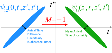
Figure 1: (color online). Two-dimensional sketches of the two-photon probability amplitude before and after one of the photons is time-reversed. Uncertainty in arrival time difference is transformed to uncertainty in mean arrival time.

The most interesting case is when $M=-1$, and one of the photons is time-reversed. If the two photons are initially entangled with positive time correlation, $\psi_{12}$ can be written as

$$\psi_{12}(0,t,z^{\prime},t^{\prime}) =a(t)b(t-t^{\prime}),$$ (41)

where $b$ is assumed to be much sharper than $a$. After photon 1 has passed through the temporal imaging system with $M=-1$,

$$\psi_{12}(z,t,z^{\prime},t^{\prime}) =a(t_{d}-t)b(t_{d}-t-t^{\prime}).$$ (42)

The photons hence become anti-correlated in time. See Fig. 1 for an illustration of this process. Since most conventional two-photon sources generate positive time correlation, but negative time correlation is desirable for many applications, one can use the temporal imaging system to convert the former to the latter. In particular, using the aforementioned technique for the specific application of clock synchronization, the sub-classical uncertainty of arrival time difference, $(t-t^{\prime})/2$, can be converted to a sub-classical uncertainty of mean arrival time, $(t+t^{\prime})/2$, leading to a quantum enhancement of clock synchronization accuracy by a factor of $\sqrt{2}$ over the classical limit. In practice, the clock can be synchronized with the electro-optic modulator, so that the mean arrival time is controlled by $t_{0}$ and thus the clock. The proposed setup is drawn in Fig. 2.

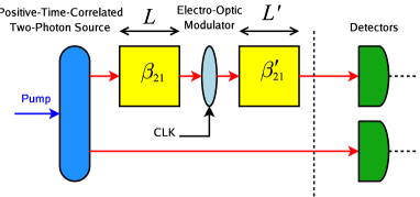
Figure 2: (color online). A quantum temporal imaging system for quantum-enhanced clock synchronization.

The fidelity of time reversal is limited by parasitic effects, such as higher-order dispersion and phase modulation, and the temporal aperture $T_{a}$, which adds a factor $\sim\beta_{21}^{\prime}L^{\prime}/T_{a}$ to the width of $\psi$ along the $t$ axis and increases the overall uncertainty of the mean arrival time. The ultimate limit, apart from instrumental ones, is set by the failure of the slowly-varying envelope approximation, which only concerns ultrashort pulses with few optical cycles.

Besides the above application, one can also convert negative time correlation, which can be generated by ultrashort pulses for improved efficiency walton ; tsangPRA ; giovannettiPRA , to positive time correlation. As evident from Eq. (38), any desired correlation can actually be imposed on already entangled photons, by multiplying the original correlation with a factor of $1/M$.

As group-velocity dispersion and temporal phase modulation play analogous roles in the time domain to diffraction and lenses, one can use Fourier optics goodman , temporal imaging kolner , and quantum imaging abouraddy techniques to design more complex quantum temporal imaging systems.

IV Two Photons in Two Linearly-Coupled Modes

Suppose that the two modes are now coupled to each other, via, for example, a beam splitter or a fiber coupler. Equations (9) and (10) become coupled-mode equations,

$$\Big{(}\frac{\partial}{\partial z}-iK_{1}\Big{)}\hat{A}_{1} =i\kappa(z)\hat{A}_{2}+\hat{F}_{1},$$ (43)

$$\Big{(}\frac{\partial}{\partial z^{\prime}}-iK_{2}^{\prime}\Big{)}\hat{A}_{2}^{\prime} =i\kappa^{*}(z^{\prime})\hat{A}_{1}^{\prime}+\hat{F}_{2}^{\prime},$$ (44)

where $\kappa$ is the coupling coefficient, and for simplicity the coupling is assumed to be co-directional. The primes denote the evaluations of the functions at $(z^{\prime},t^{\prime})$. Any phase mismatch can be incorporated into $\kappa$ as a $z$-dependent phase.

Procedures similar to those in Sec. II produce four coupled equations for $\psi_{11}$, $\psi_{22}$, and $\psi_{12}$,

$$\Big{(}\frac{\partial}{\partial z}-iK_{1}\Big{)}\sqrt{2}\psi_{11}(z,t,z^{\prime},t^{\prime}) =i\kappa\psi_{12}(z^{\prime},t^{\prime},z,t),$$ (45)

$$\Big{(}\frac{\partial}{\partial z^{\prime}}-iK_{2}^{\prime}\Big{)}\sqrt{2}\psi_{22}(z,t,z^{\prime},t^{\prime}) =i{\kappa^{*}}^{\prime}\psi_{12}(z^{\prime},t^{\prime},z,t),$$ (46)

$$\Big{(}\frac{\partial}{\partial z}-iK_{1}\Big{)}\psi_{12}(z,t,z^{\prime},t^{\prime}) =i\kappa\sqrt{2}\psi_{22}(z,t,z^{\prime},t^{\prime}),$$ (47)

$$\Big{(}\frac{\partial}{\partial z^{\prime}}-iK_{2}^{\prime}\Big{)}\psi_{12}(z,t,z^{\prime},t^{\prime}) =i{\kappa^{*}}^{\prime}\sqrt{2}\psi_{11}(z,t,z^{\prime},t^{\prime}).$$ (48)

Any pair of Eqs. (46) and (47) or Eqs. (45) and (48) can be combined to yield a single equation for $\psi_{12}$,

$$\quad\Big{(}\frac{\partial}{\partial z}-iK_{1}\Big{)}\Big{(}\frac{\partial}{\partial z^{\prime}}-iK_{2}^{\prime}\Big{)}\psi_{12}(z,t,z^{\prime},t^{\prime})$$

$$=-\kappa(z)\kappa^{*}(z^{\prime})\psi_{12}(z^{\prime},t^{\prime},z,t).$$ (49)

Equation (49) allows one to calculate the coupled-mode propagation of two photons in terms of $\psi_{12}$ only, given the initial conditions of $\psi_{12}$, $\psi_{11}$, and $\psi_{22}$. $\psi_{11}$ and $\psi_{22}$ can then be obtained from Eqs. (47) and (48) after $\psi_{12}$ is calculated.

To obtain some insight into Eq. (49), consider only constant mode coupling, so that Eq. (49) becomes

$$\frac{\partial}{\partial z}\frac{\partial}{\partial z^{\prime}}\psi_{12}(z,t,z^{\prime},t^{\prime}) =-\kappa^{2}\psi_{12}(z^{\prime},t^{\prime},z,t).$$ (50)

The solution is

$$\psi_{12}(z,t,z^{\prime},t^{\prime}) =\cos(\kappa z)\cos(\kappa z^{\prime})\psi_{12}(0,t,0,t^{\prime})-$$

$$\quad\sin(\kappa z)\sin(\kappa z^{\prime})\psi_{12}(0,t^{\prime},0,t)+$$

$$\quad i\sin(\kappa z)\cos(\kappa z^{\prime})\sqrt{2}\psi_{22}(0,t,0,t^{\prime})+$$

$$\quad i\cos(\kappa z)\sin(\kappa z^{\prime})\sqrt{2}\psi_{11}(0,t,0,t^{\prime}).$$ (51)

At the coupler output, $z=z^{\prime}=L$,

$$\psi_{12}(L,t,L,t^{\prime}) =T\psi_{12}(0,t,0,t^{\prime})-R\psi_{12}(0,t^{\prime},0,t)+$$

$$\quad i\sqrt{2TR}\psi_{22}(0,t,0,t^{\prime})+$$

$$\quad i\sqrt{2TR}\psi_{11}(0,t,0,t^{\prime}).$$ (52)

where $T=\cos^{2}(\kappa L)$ and $R=1-T=\sin^{2}(\kappa L)$. If we have one photon in each mode initially, only the initial condition of $\psi_{12}$ is non-zero, and

$$\psi_{12}(L,t,L,t^{\prime}) =T\psi_{12}(0,t,0,t^{\prime})-R\psi_{12}(0,t^{\prime},0,t).$$ (53)

From Eq. (53), one can see that the output amplitude is the destructive interference between the original amplitude and its replica but with the two photons exchanging their positions in time. In particular, for a 50%-50% coupler, $T=R=1/2$, complete destructive interference is produced if the two input photons are temporally indistinguishable. See Fig. 3 for a graphical illustration of the destruction interference. The introduction of variable distinguishability to photons, in order to produce varying degrees of destructive interference of $\psi_{12}$ via a beam splitter and to measure the two-photon coherence time, is the basic principle of the Hong-Ou-Mandel interferometer hom .

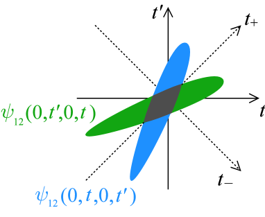
Figure 3: (color online). The quantum destructive interference via a coupler is determined by the overlap (dark grey area) of the two-photon amplitude $\psi_{12}(0,t,0,t^{\prime})$ with its mirror image with respect to the $t+t^{\prime}$ axis, $\psi_{12}(0,t^{\prime},0,t)$.

V Two Photons in Many Modes

If the two photons are optically coupled to more than two modes, such as four modes for two polarizations in each of the two propagation directions, or $N$ modes in an array of $N$ fibers coupled to each other, one in general needs $N(N+1)/2$ two-photon amplitudes to describe the system. The propagation of the amplitudes in many modes is described by the following,

$$\quad\Big{(}\frac{\partial}{\partial z}-iK_{j}\Big{)}\sqrt{1+\delta_{jk}}\psi_{jk}(z,t,z^{\prime},t^{\prime})$$

$$=i\sum_{l\neq j}\kappa_{jl}\sqrt{1+\delta_{lk}}\psi_{lk}(z,t,z^{\prime},t^{\prime}),$$ (54)

where

$$\psi_{jk}(z,t,z^{\prime},t^{\prime}) =\psi_{kj}(z^{\prime},t^{\prime},z,t),\quad\kappa_{jk}=\kappa_{kj}^{*}.$$ (55)

Further simplications can also be made if any of the coupling terms is zero.

For example, let there be four modes; mode 1 corresponds to arm 1 with $x$ polarization, mode 2 corresponds to arm 2 with $x$ polarization, mode 3 corresponds to arm 1 with $y$ polarization, and mode 4 corresponds to arm 2 with $y$ polarization. If only the same polarizations are coupled, the two-photon equations are

$$\left(\begin{array}[]{cccc}\frac{\partial}{\partial z}&-i\kappa_{x}&0&0\\ -i\kappa_{x}&\frac{\partial}{\partial z}&0&0\\ 0&0&\frac{\partial}{\partial z}&-i\kappa_{y}\\ 0&0&-i\kappa_{y}&\frac{\partial}{\partial z}\end{array}\right)\times$$ (60)

$$\left(\begin{array}[]{cccc}\sqrt{2}\psi_{11}&\psi_{12}&\psi_{13}&\psi_{14}\\ \psi_{21}&\sqrt{2}\psi_{22}&\psi_{23}&\psi_{24}\\ \psi_{31}&\psi_{32}&\sqrt{2}\psi_{33}&\psi_{34}\\ \psi_{41}&\psi_{42}&\psi_{43}&\sqrt{2}\psi_{44}\end{array}\right)=0.$$ (65)

The following solution for the orthogonally polarized amplitudes can be obtained,

$$\quad\left(\begin{array}[]{c}\psi_{13}(L,t,L,t^{\prime})\\ \psi_{24}(L,t,L,t^{\prime})\\ \psi_{14}(L,t,L,t^{\prime})\\ \psi_{23}(L,t,L,t^{\prime})\end{array}\right)$$ (70)

$$=\left(\begin{array}[]{cccc}\sqrt{T_{x}T_{y}}&-\sqrt{R_{x}R_{y}}&i\sqrt{T_{x}R_{y}}&i\sqrt{T_{y}R_{x}}\\ -\sqrt{R_{x}R_{y}}&\sqrt{T_{x}T_{y}}&i\sqrt{T_{y}R_{x}}&i\sqrt{T_{x}R_{y}}\\ i\sqrt{T_{x}R_{y}}&i\sqrt{T_{y}R_{x}}&\sqrt{T_{x}T_{y}}&-\sqrt{R_{x}R_{y}}\\ i\sqrt{T_{y}R_{x}}&i\sqrt{T_{x}R_{y}}&-\sqrt{R_{x}R_{y}}&\sqrt{T_{x}T_{y}}\end{array}\right)\times$$ (75)

$$\quad\left(\begin{array}[]{c}\psi_{13}(0,t,0,t^{\prime})\\ \psi_{24}(0,t,0,t^{\prime})\\ \psi_{14}(0,t,0,t^{\prime})\\ \psi_{23}(0,t,0,t^{\prime})\end{array}\right),$$ (80)

where $T_{x,y}=\cos^{2}(\kappa_{x,y}L)$ and $R_{x,y}=1-T_{x,y}$. In particular, if only the initial condition of $\psi_{14}$ is non-zero,

$$\psi_{13}(L,t,L,t^{\prime}) =i\sqrt{T_{x}R_{y}}\psi_{14}(0,t,0,t^{\prime}),$$ (81)

$$\psi_{24}(L,t,L,t^{\prime}) =i\sqrt{T_{y}R_{x}}\psi_{14}(0,t,0,t^{\prime}),$$ (82)

$$\psi_{14}(L,t,L,t^{\prime}) =\sqrt{T_{x}T_{y}}\psi_{14}(0,t,0,t^{\prime}),$$ (83)

$$\psi_{23}(L,t,L,t^{\prime}) =-\sqrt{R_{x}R_{y}}\psi_{14}(0,t,0,t^{\prime}).$$ (84)

The singlet state for orthogonally polarized photons is produced if $T_{x}=T_{y}=1/2$ ohm .

VI Four-Wave Mixing

As envisioned by Lukin et al., the third-order nonlinear effects among two photons can become significant in a coherently prepared atomic gas lukin . The coupled-mode equations (43) and (44) then become nonlinear,

$$\Big{(}\frac{\partial}{\partial z}-iK_{1}\Big{)}\hat{A}_{1} =i\kappa\hat{A}_{2}+i\gamma\hat{A}_{1}^{\dagger}\hat{A}_{1}\hat{A}_{1}+i\eta\hat{A}_{2}^{\dagger}\hat{A}_{2}\hat{A}_{1}+$$

$$\quad i\chi\hat{A}_{2}\hat{A}_{2}\hat{A}_{1}^{\dagger}+\hat{F}_{1},$$ (85)

$$\Big{(}\frac{\partial}{\partial z^{\prime}}-iK_{2}^{\prime}\Big{)}\hat{A}_{2}^{\prime} =i{\kappa^{*}}^{\prime}\hat{A}_{1}^{\prime}+i\gamma\hat{A^{\prime}}_{2}^{\dagger}\hat{A}_{2}^{\prime}\hat{A}_{2}^{\prime}+i\eta\hat{A^{\prime}}_{1}^{\dagger}\hat{A}_{1}^{\prime}\hat{A}_{2}^{\prime}+$$

$$\quad i{\chi^{*}}^{\prime}\hat{A}_{1}^{\prime}\hat{A}_{1}^{\prime}\hat{A^{\prime}}_{2}^{\dagger}+\hat{F}_{2}^{\prime},$$ (86)

where $\gamma$ is the self-phase modulation coefficient, $\eta$ is the cross-phase modulation coefficient, and $\chi$ is the four-wave mixing coefficient. If we define equal-space two-photon amplitudes as the following,

$$\psi_{jk}(z,t,t^{\prime}) =\psi_{jk}(z,t,z,t^{\prime}),$$ (87)

three linear coupled-mode equations for the two-photon amplitudes can be derived,

$$\Big{(}\frac{\partial}{\partial z}-iK_{1}-iK_{1}^{\prime}\Big{)}\sqrt{2}\psi_{11} =i\kappa\psi_{21}+i\gamma\delta(t-t^{\prime})\sqrt{2}\psi_{11}+$$

$$\quad i\chi\delta(t-t^{\prime})\sqrt{2}\psi_{22},$$ (88)

$$\Big{(}\frac{\partial}{\partial z}-iK_{2}-iK_{2}^{\prime}\Big{)}\sqrt{2}\psi_{22} =i{\kappa^{*}}\psi_{21}+i\gamma\delta(t-t^{\prime})\sqrt{2}\psi_{22}+$$

$$\quad i\chi^{*}\delta(t-t^{\prime})\sqrt{2}\psi_{11},$$ (89)

$$\Big{(}\frac{\partial}{\partial z}-iK_{1}-iK_{2}^{\prime}\Big{)}\psi_{12} =i\kappa^{*}\sqrt{2}\psi_{11}+i\kappa\sqrt{2}\psi_{22}+$$

$$\quad i\eta\delta(t-t^{\prime})\psi_{12}.$$ (90)

The advantage of the Schrödinger picture is most evident here; whereas in the Heisenberg picture one needs to solve nonlinear coupled-mode operator equations such as Eqs. (85) and (86), in the Schrödinger picture, one only needs to solve linear equations such as Eqs. (88) to (90), which are similar to the configuration-space model applied to the quantum theory of solitons lai ; hagelstein .

The delta function $\delta(t-t^{\prime})$ couples the two subspaces of $\psi_{12}(z,t,t^{\prime})$, so entanglement can emerge from unentangled photons lukin . To see this effect, assume that we only have four-wave mixing, so that Eq. (90) becomes

$$\frac{\partial}{\partial z}\psi_{12}(z,t,t^{\prime}) =i\eta\delta(t-t^{\prime})\psi_{12}(z,t,t^{\prime}),$$ (91)

which yields

$$\psi_{12}(L,t,t^{\prime}) =\exp[i\eta L\delta(t-t^{\prime})]\psi_{12}(0,t,t^{\prime}).$$ (92)

If the nonlinearity has a finite bandwidth $\Delta\omega$, the delta function in time should be replaced by a finite-bandwidth function, for example a sinc function,

$$\psi_{12}(L,t,t^{\prime}) =\exp\Big{\{}\frac{i\eta L}{\pi(t-t^{\prime})}\sin\Big{[}\frac{\Delta\omega}{2}(t-t^{\prime})\Big{]}\Big{\}}\times$$

$$\quad\psi_{12}(0,t,t^{\prime}).$$ (93)

Eq. (93) is the exact solution of the two-photon amplitude under the cross-phase modulation effect, while Eq. (7) in Ref. lukin , presumably derived in the Heisenberg picture, is only correct in the first-order. As $\psi_{12}(L,t,t^{\prime})$ cannot be written as a product of one-photon amplitudes even if the two photons are initially unentangled, entanglement is generated. The physical interpretation is that the two input photons act as pump photons to the spontaneous four-wave mixing process and are annihilated to generate two new entangled photons.

Unlike temporal imaging techniques, which can only manipulate the two-photon amplitude along the horizontal axis $t$ or the vertical axis $t^{\prime}$, cross-phase modulation allows some manipulation of the two-photon amplitude along the diagonal time-difference axis, $t-t^{\prime}$. Unfortunately, cross-phase modulation by itself cannot generate any temporal correlation, as it only imposes a phase on the two-photon temporal amplitude. In order to have more control along the $t-t^{\prime}$ axis, one can combine the effects of cross-phase modulation and dispersion, as shown in the following section.

VII Two-Photon Vector Solitons

In this section we study a toy example, namely, a soliton formed by two photons in orthogonal polarizations exerting cross-phase modulation on each other agrawal . Although similar studies of two photons in the same mode under the self-phase modulation effect have been performed in Refs. chiao , cross-phase modulation offers the distinct possibility of entangling two photons in different modes.

Consider the case in which two polarizations have the same group-velocity dispersion, so that $\beta_{21}=\beta_{22}=\beta_{2}$, and there is one photon in each polarization. The evolution equation for $\psi_{12}(z,t,t^{\prime})$ is

$$\quad\Big{(}\frac{\partial}{\partial z}+\beta_{11}\frac{\partial}{\partial t}+\beta_{12}\frac{\partial}{\partial t^{\prime}}\Big{)}\psi_{12}$$

$$=\Big{[}-\frac{i\beta_{2}}{2}\Big{(}\frac{\partial^{2}}{\partial t^{2}}+\frac{\partial^{2}}{\partial t^{\prime 2}}\Big{)}+i\eta\delta(t-t^{\prime})\Big{]}\psi_{12}.$$ (94)

Defining time coordinates in a moving frame,

$$\tau =t-\bar{\beta}_{1}z, \tau^{\prime} =t^{\prime}-\bar{\beta}_{1}z,$$ (95)

$$\bar{\beta}_{1} =\frac{\beta_{11}+\beta_{12}}{2}, \Delta =\frac{\beta_{11}-\beta_{12}}{2},$$ (96)

we obtain the following equation for $\psi_{12}(z,\tau,\tau^{\prime})$,

$$\quad\Big{(}\frac{\partial}{\partial z}+\Delta\frac{\partial}{\partial\tau}-\Delta\frac{\partial}{\partial\tau^{\prime}}\Big{)}\psi_{12}$$

$$=\Big{[}-\frac{i\beta_{2}}{2}\Big{(}\frac{\partial^{2}}{\partial\tau^{2}}+\frac{\partial^{2}}{\partial\tau^{\prime 2}}\Big{)}+i\eta\delta(\tau-\tau^{\prime})\Big{]}\psi_{12}.$$ (97)

Equation (97) is a simple linear Schrödinger equation, describing a two-dimensional “wavefunction” $\psi_{12}(z,\tau,\tau^{\prime})$ in a moving frame subject to a delta potential. To solve for $\psi_{12}$ explicity, we define new time coordinates,

$$\tau_{+} =\frac{\tau+\tau^{\prime}}{2},\quad\tau_{-}=\frac{\tau-\tau^{\prime}}{2},$$ (98)

Eq. (97) then becomes

$$\quad\Big{(}\frac{\partial}{\partial z}+\Delta\frac{\partial}{\partial\tau_{-}}\Big{)}\psi_{12}$$

$$=\Big{[}-\frac{i\beta_{2}}{4}\Big{(}\frac{\partial^{2}}{\partial\tau_{+}^{2}}+\frac{\partial^{2}}{\partial\tau_{-}^{2}}\Big{)}+\frac{i\eta}{2}\delta(\tau_{-})\Big{]}\psi_{12}.$$ (99)

As evident from Eq. (99), the cross-phase modulation effect only offers confinement of $\psi_{12}$ along the time difference ($\tau_{-}$) axis, but not the mean arrival time ($\tau_{+}$) axis.

The only bound-state solution of $\psi_{12}$ is

$$\quad\psi_{12}(z,\tau_{+},\tau_{-})$$

$$=\exp\Big{[}-i\Big{(}\frac{\beta_{2}}{4}S^{2}+\frac{\Delta^{2}}{\beta_{2}}\Big{)}z\Big{]}\times$$

$$\quad\exp\Big{(}-S|\tau_{-}|+i\frac{2\Delta}{\beta_{2}}\tau_{-}\Big{)}\times$$

$$\quad\int_{-\infty}^{\infty}\frac{d\Omega}{2\pi}\mbox{ }\phi(\Omega)\exp\Big{(}-i\Omega\tau_{+}+\frac{i\beta_{2}}{4}\Omega^{2}z\Big{)}.$$ (100)

The delta potential enforces $S$ to take on the following value,

$$S =-\frac{\eta}{\beta_{2}},$$ (101)

where $\eta$ and $\beta_{2}$ must have opposite signs. The final solution of $\psi_{12}$ in the frame of $\tau$ and $\tau^{\prime}$ is therefore

$$\quad\psi_{12}(z,\tau,\tau^{\prime})$$

$$=\exp\Big{[}-i\Big{(}\frac{\eta^{2}/4+\Delta^{2}}{\beta_{2}}\Big{)}z\Big{]}\times$$

$$\quad\exp\Big{[}-\Big{|}\frac{\eta}{2\beta_{2}}\Big{|}|\tau-\tau^{\prime}|+i\frac{\Delta}{\beta_{2}}(\tau-\tau^{\prime})\Big{]}\times$$

$$\quad\int_{-\infty}^{\infty}\frac{d\Omega}{2\pi}\mbox{ }\phi(\Omega)\exp\Big{[}-i\Omega(\frac{\tau+\tau^{\prime}}{2})+\frac{i\beta_{2}}{4}\Omega^{2}z\Big{]}.$$ (102)

The two-photon coherence time of a vector soliton is fixed, but the average arrival time is still subject to dispersive spreading and becomes increasingly uncertain as they propagate. See Fig. 4 for an illustration. Hence, a two-photon vector soliton generates temporal entanglement with positive time correlation as it propagates. Similar to the idea of soliton momentum squeezing fini , one can also adiabatically change $\eta$ or $\beta_{2}$ along the propagation axis to control independently the two-photon coherence time.

Notice that the center frequencies of the two photons are shifted slightly, by an amount of $\pm\Delta/\beta_{2}$, to compensate for their group-velocity mismatch, so that they can co-propagate at the average group velocity. This is commonly known as soliton trapping agrawal .

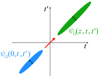
Figure 4: (color online). Quantum dispersive spreading of mean arrival time of a two-photon vector soliton. The cross-phase modulation effect only preserves the two-photon coherence time, giving rise to temporal entanglement with positive time correlation. One can also manipulate the coherence time independently by adiabatically changing the nonlinear coefficient along the propagation axis.

If the nonlinearity has a finite bandwidth, then the potential becomes a finite-bandwidth function like the one in Eq. (93), and multiple bound-state solutions can be obtained via conventional techniques of solving the linear Schrödinger equation.

VIII Conclusion

We have derived the general equations that govern the temporal evolution of two-photon probability amplitudes in different coupled optical modes. The formalism inspires the concept of quantum temporal imaging, which can manipulate the temporal entanglement of photons via conventional imaging techniques. The theory also offers an intuitive interpretation of two-photon entanglement evolution, as demonstrated by the exact solution of a two-photon vector soliton. To conclude, we expect the proposed formalism to be useful for many quantum signal processing and communication applications.

IX Acknowledgements

This work was supported by the Engineering Research Centers Program of the National Science Foundation under Award Number EEC-9402726 and the Defense Advanced Research Projects Agency (DARPA).

References

• (1) Y. Lai and H. A. Haus, Phys. Rev. A40, 844 (1989), Y. Lai and H. A. Haus, Phys. Rev. A40, 854 (1989).
• (2) B. E. A. Saleh, M. C. Teich, and A. V. Sergienko, Phys. Rev. Lett. 94, 223601 (2005).
• (3) E. Wolf, Nuovo Cimento 12, 884 (1954).
• (4) M. D. Lukin and A. Imamoglu, Phys. Rev. Lett. 84, 1419 (2000).
• (5) J. D. Franson, Phys. Rev. A45, 3126 (1992).
• (6) A. M. Steinberg, P. G. Kwiat and R. Y. Chiao, Phys. Rev. A45, 6659 (1992).
• (7) C. K. Hong, Z. Y. Ou, and L. Mandel, Phys. Rev. Lett. 59, 2044 (1987).
• (8) R. Y. Chiao, I. H. Deutsch, and J. C. Garrison, Phys. Rev. Lett. 67, 1399 (1991), I. H. Deutsch, R. Y. Chiao, and J. C. Garrison, Phys. Rev. Lett. 69 3627 (1992).
• (9) V. Giovannetti, S. Lloyd, and L. Maccone, Nature (London)412, 417 (2001).
• (10) V. Giovannetti, L. Maccone, J. H. Shapiro, and F. N. C. Wong, Phys. Rev. Lett. 88, 183602 (2002).
• (11) Z. D. Walton, M. C. Booth, A. V. Sergienko, B. E. A. Saleh, and M. C. Teich, Phys. Rev. A67, 053810 (2003).
• (12) J. P. Torres, F. Macia, S. Carrasco, and L. Torner, Opt. Lett. 30, 314 (2005).
• (13) M. Tsang and D. Psaltis, Phys. Rev. A71, 043806 (2005).
• (14) O. Kuzucu, M. Fiorentino, M. A. Albota, F. N. C. Wong, and F. X. Kärtner, Phys. Rev. Lett. 94, 083601 (2005).
• (15) B. Huttner and S. M. Barnett, Phys. Rev. A46, 4306 (1992).
• (16) R. Matloob, R. Loudon, S. M. Barnett, and J. Jeffers, Phys. Rev. A52, 4823 (1995).
• (17) G. P. Agrawal, Nonlinear Fiber Optics (Academic Press, San Diego, 2001).
• (18) M. H. Rubin, D. N. Klyshko, Y. H. Shih, and A. V. Sergienko, Phys. Rev. A50, 5122 (1994).
• (19) M. Fiorentino, P. L. Voss, J. E. Sharping, and P. Kumar, IEEE Photon. Tech. Lett. 14, 983 (2002).
• (20) J. Jeffers and S. M. Barnett, Phys. Rev. A47, 3291 (1993).
• (21) B. H. Kolner and M. Nazarathy, Opt. Lett. 14, 630 (1989), B. H. Kolner, IEEE J. Quantum Electron. 30, 1951 (1994).
• (22) V. Giovannetti, L. Maccone, J. H. Shapiro, and F. N. C. Wong, Phys. Rev. A66, 043813 (2002).
• (23) J. W. Goodman, Introduction to Fourier Optics (McGraw-Hill, Boston, 1996).
• (24) A. F. Abouraddy, B. E. A. Saleh, A. V. Sergienko, and M. C. Teich, J. Opt. Soc. Am. B19, 1174 (2002).
• (25) Z. Y. Ou, C. K. Hong, and L. Mandel, Opt. Commun. 63, 118 (1987).
• (26) P. L. Hagelstein, Phys. Rev. A54, 2426 (1996).
• (27) J. M. Fini and P. L. Hagelstein, Phys. Rev. A66, 033818 (2002).