Quantum Fluctuations of Coulomb Potential as a Source of Flicker Noise.
The Influence of External Electric Field

Abstract

Fluctuations of the electromagnetic field produced by quantized matter in external electric field are investigated. A general expression for the power spectrum of fluctuations is derived within the long-range expansion. It is found that in the whole measured frequency band, the power spectrum of fluctuations exhibits an inverse frequency dependence. A general argument is given showing that for all practically relevant values of the electric field, the power spectrum of induced fluctuations is proportional to the field strength squared. As an illustration, the power spectrum is calculated explicitly using the kinetic model with the relaxation-type collision term. Finally, it is shown that the magnitude of fluctuations produced by a sample generally has a Gaussian distribution around its mean value, and its dependence on the sample geometry is determined. In particular, it is demonstrated that for geometrically similar samples, the power spectrum is inversely proportional to the sample volume. Application of the obtained results to the problem of flicker noise is discussed.

I Introduction

As is well-known, power spectra of voltage fluctuations in all conducting materials exhibit a universal profile in the low-frequency limit, which is close to inverse frequency dependence. Fluctuations characterized by the power spectrum of this type are called usually $1/f,$ or flicker, noise. Although this noise dominates only at low frequencies, experiments show the presence of the $1/f$-component in the whole measured frequency band up to $10^{6}Hz.$ Despite numerous attempts, no lower frequency bound for the $1/f$ law has been found. In addition to that, it is generally accepted that $1/f$-noise produced by a sample is universally characterized by the following properties 1) it is (roughly) inversely proportional to the sample volume, 2) it is Gaussian, and 3) its part induced by external electric field is proportional to the field strength squared.

A number of mechanisms has been suggested to explain the origin of $1/f$-noise buck . There is a widespread opinion that this noise arises from resistance fluctuations, which is quite natural taking into account the property 3) mentioned above. Indeed, for a given current through the sample, the mean squares of voltage and resistance fluctuations are proportional to each other, the current squared being the proportionality coefficient. It has been proposed that the resistance fluctuations possessing the other properties of flicker noise might result from temperature fluctuations voss , fluctuations in the carrier mobility hooge ; klein or in the number of carriers caused by surface traps mcwhorter . All these models, however, have restricted validity, because they involve one or another assumption specific to the problem under consideration. For instance, assuming that the resistance fluctuations arise from the temperature fluctuations, one has to choose an appropriate spatial correlation of these fluctuations in order to obtain the desired profile of the power spectrum. Similarly, the model of Ref. mcwhorter requires specific distribution of trapping times. In addition to that, the models proposed so far reproduce the $1/f$-profile only in a restricted range of frequencies, require an appropriate normalization of the power spectrum, etc. At the same time, ubiquity of flicker noise and universality of its properties suggest existence of a simple and universal, and therefore, fundamental origin. It is natural to look for this reason in the quantum properties of charge carriers. In this direction, the problem has been extensively investigated by Handel and co-workers handel . Handel’s approach is based on the theory of infrared radiative corrections in quantum electrodynamics. Handel showed that the $1/f$ power spectrum of photons emitted in any scattering process can be derived from the well-know property of bremsstrahlung, namely, from the infrared divergence of the cross-section considered as a function of the energy loss. Thus, this theory treats the $1/f$-noise as a relativistic effect (in fact, the noise level in this theory $\sim\alpha(\Delta\bm{v})^{2}/c^{2},$ where $\alpha$ is the fine structure constant, $\Delta\bm{v}$ velocity change of the particle being scattered, and $c$ the speed of light). It should be mentioned, however, that the Handel’s theory has been severely criticized in many respects tremblay ; kampen .

In Refs. kazakov1 ; kazakov , the role of quantum effects is considered from a purely nonrelativistic point of view. In Ref. kazakov1 , quantum fluctuations of the electromagnetic field produced by elementary particles are investigated, and it is shown, in particular, that the correlation function of the fluctuations exhibits an inverse frequency dependence in the low-frequency limit. This result was applied in Ref. kazakov to the calculation of the power spectrum of electromagnetic fluctuations produced by a sample. It was proved, in particular, that the power spectrum possesses the properties 1), 2) of flicker noise, mentioned above. As to the property 3), it was argued in Ref. kazakov that this requirement is also met. The argument was based on the assumption of analyticity of the electron density matrix with respect to the external electric field. However, this assumption is not valid in general. Thus, the issue concerning the influence of external field is left open.

The purpose of the present paper is to investigate the influence of the external electric field on quantum electromagnetic fluctuations in detail. We will show that for all practically relevant values of the field strength, the power spectrum of induced fluctuations is proportional to the field strength squared indeed.

Inclusion of an external field lowers the system symmetry, therefore, our first problem below will be to generalize the results obtained in kazakov for spherically-symmetric systems to systems with axial symmetry. This is done in Sec. III. First of all, we prove in Sec. III.1 that the low-frequency asymptotic of the connected part of correlation function is logarithmic. This result was proved already in kazakov . Although the proof does not rely on the system symmetries, we give an independent and more simple and accurate proof of this important fact. Contribution of the disconnected part is calculated in Sec. III.2, and is found to exhibits an inverse frequency dependence, thus dominating in the low-frequency limit. Because of the lower system symmetry, this calculation is much more complicated than in the case considered in kazakov . The obtained expression for the power spectrum is analyzed in Sec. IV where a general argument is given showing that the field-induced noise is quadratic in the field strength, which is then illustrated using the simplest kinetic model with the relaxation-type collision term. Section V summarizes the results of the work and states the conclusion.

II Preliminaries

Let us consider electromagnetic field produced by a classical resting particle with mass $m$ and electric charge $e.$ It is described by the Coulomb potential

$$A_{0}=\frac{e}{4\pi r}\,,\qquad\bm{A}=0\,.$$ (1)

In quantum theory, this form of the electromagnetic potential is reproduced by the mean fields $\langle{\rm in}|\hat{A}_{0}|{\rm in}\rangle,$ $\langle{\rm in}|\hat{\bm{A}}|{\rm in}\rangle$ calculated far away from the region of particle localization. If the 3-vector of the mean particle position is denoted by $\bm{x}_{0},$ and that of the point of observation by $\bm{x},$ then the latter condition means that $|\bm{x}-\bm{x}_{0}|\gg D,$ where $D$ is a characteristic length of the particle wave packet spatial spreading (for instance, the variance of the particle coordinates). As a result of the quantum evolution according to the Schrodinger equation, $D$ increases in time, thus leading to a dispersion of the electromagnetic field produced by the particle. Furthermore, because of the quantum indeterminacy in the particle position, the field fluctuates. The correlation function of the fluctuations is conventionally defined by

$$C_{\mu\nu}(x,x^{\prime})=\frac{1}{2}\langle{\rm in}|\hat{A}_{\mu}(x)\hat{A}_{\nu}(x^{\prime})+\hat{A}_{\nu}(x^{\prime})\hat{A}_{\mu}(x)|{\rm in}\rangle-\langle{\rm in}|\hat{A}_{\mu}(x)|{\rm in}\rangle\langle{\rm in}|\hat{A}_{\nu}(x^{\prime})|{\rm in}\rangle\,,$$ (2)

where $x$ and $x^{\prime}$ are the spacetime coordinates of two observation points. Of course, this function is dispersed, too. Our aim below will be to investigate low-frequency properties of this dispersion. It is clear that the condition $|\bm{x}-\bm{x}_{0}|\gg D$ is irrelevant in this investigation, because the low-frequency asymptotic of the power spectrum of correlations is determined largely by the late-time behavior of the function $C_{\mu\nu}(x,x^{\prime}),$ where $D$ is unbounded (for a free particle state, and for large times $t,$ $D$ is a linear function of $t$).

As in Ref. kazakov , we will work within the long-range expansion of the correlation function, which is a convenient tool for extracting the leading term of the correlation function. Let us briefly recall the reasons justifying application of this expansion. The function $C_{\mu\nu}(x,x^{\prime})$ can be represented as a power series in the ratios $l_{c}/R$ and $D/R,$ where $l_{c}=\hbar/mc$ is the Compton length, and $R$ is either $r=|\bm{x}-\bm{x}_{0}|$ or $r^{\prime}=|\bm{x}^{\prime}-\bm{x}_{0}|.$ However, as mentioned above, the ratio $D/R$ cannot be considered small as long as one is concerned with the low-frequency behavior of correlations. We overcome this problem by going over to the momentum space, and work with an expansion in powers of $l_{c}$ and $\bm{p}/\tilde{D},$ where $\bm{p}$ is the 3-momentum transfer to the particle, and $\tilde{D}=\sqrt{\langle\bm{q}^{2}\rangle}$ is the variance of the particle momentum. Unlike $D,$ the quantity $\tilde{D}$ is time independent (for free particle states), so the expansion is valid for all times. By the order of magnitude, the relevant values of the momentum transfer $|\bm{p}|\sim\hbar/r,$ and therefore, validity of the expansion in powers of $\bm{p}/\tilde{D}$ requires only that

$$r\tilde{D}\gg\hbar\,,\quad r^{\prime}\tilde{D}\gg\hbar\,.$$

All subsequent considerations are carried out under these conditions.

We recall also that, as was shown in Ref. kazakov1 , the leading term of the correlation function is of zeroth order in $l_{c},$ hence, in the units $\hbar=c=1$ used from now on, it can be identified as the limit of the correlation function for $m\to\infty.$ It should be emphasized that this identification is only formal, in particular, it does not mean that the results obtained below apply only to heavy particles.

According to Eq. (2), in order to find the correlation function of the electromagnetic fluctuations, one has to calculate the in-in expectation values of the field operators $\hat{A}_{\mu}$ as well as of their products. In Refs. kazakov1 ; kazakov , this was done using the Schwinger-Keldysh formalism. In particular, it was proved in Ref. kazakov that the leading low-frequency term of the correlation function is contained entirely in its disconnected part [the second term in Eq. (2)]. The connected part of the correlation function was taken in Ref. kazakov in the nonsymmetric form $\langle{\rm in}|\hat{A}_{\mu}(x)\hat{A}_{\nu}(x^{\prime})|{\rm in}\rangle.$ Although the proof given there can be carried over to the present case, we will give an independent and more accurate proof of this important fact, which avoids complications of the Schwinger-Keldysh method.

Note first of all, that for all values of $t,t^{\prime},$ the connected part of the correlation function can be rewritten as

$$\frac{1}{2}\langle{\rm in}|\hat{A}_{\mu}(x)\hat{A}_{\nu}(x^{\prime})+\hat{A}_{\nu}(x^{\prime})\hat{A}_{\mu}(x)|{\rm in}\rangle=\frac{1}{2}\langle{\rm in}|T\{\hat{A}_{\mu}(x)\hat{A}_{\nu}(x^{\prime})\}+\tilde{T}\{\hat{A}_{\mu}(x)\hat{A}_{\nu}(x^{\prime})\}|{\rm in}\rangle\,,$$

where the operation of time ordering $T$ ($\tilde{T}$) arranges the factors so that the time arguments decrease (increase) from left to right. Furthermore, for a one-particle state under stationary external conditions, the state vector $|{\rm in}\rangle$ can be substituted by the vector $|{\rm out}\rangle,$ up to a phase factor. In the tree approximation, this factor is equal to unity, therefore, one can write, taking into account that $\hat{A}_{\mu}$ is Hermitian,

$$\frac{1}{2}\langle{\rm in}|\hat{A}_{\mu}(x)\hat{A}_{\nu}(x^{\prime})+\hat{A}_{\nu}(x^{\prime})\hat{A}_{\mu}(x)|{\rm in}\rangle=\frac{1}{2}\langle{\rm out}|T\{\hat{A}_{\mu}(x)\hat{A}_{\nu}(x^{\prime})\}|{\rm in}\rangle$$

$$+\frac{1}{2}\langle{\rm in}|\tilde{T}\{\hat{A}_{\mu}(x)\hat{A}_{\nu}(x^{\prime})\}|{\rm out}\rangle={\rm Re}\langle{\rm out}|T\{\hat{A}_{\mu}(x)\hat{A}_{\nu}(x^{\prime})\}|{\rm in}\rangle\,.$$ (3)

The latter quantity can be calculated by applying the usual Feynman rules.

Let us assume, for simplicity, that the field-producing particle is described by a complex scalar $\phi.$ It is not difficult to show actually that the results derived below are valid for particles of any spin. This is because in the long-range limit, the value of the electromagnetic current is fixed by the standard normalization conditions for the one-particle state, which are universal for all particle species. Let the gradient invariance be fixed by the Lorentz condition

$$G\equiv\partial^{\mu}A_{\mu}=0\,.$$ (4)

Then the action of the system takes the form

$$S[\Phi] = S_{0}[\Phi]+S_{\rm gf}[\Phi]\,,$$

$$S_{0}[\Phi] = {\displaystyle\int}d^{4}x\left\{(\partial_{\mu}\phi^{*}+ieA_{\mu}\phi^{*})(\partial^{\mu}\phi-ieA^{\mu}\phi)-m^{2}\phi^{*}\phi\right\}-\frac{1}{4}{\displaystyle\int}d^{4}xF_{\mu\nu}F^{\mu\nu}\,,$$

$$S_{\rm gf}[\Phi] = -\frac{1}{2}{\displaystyle\int}d^{4}x~{}G^{2}\,,\quad F_{\mu\nu}=\partial_{\mu}A_{\nu}-\partial_{\nu}A_{\mu}\,,$$ (5)

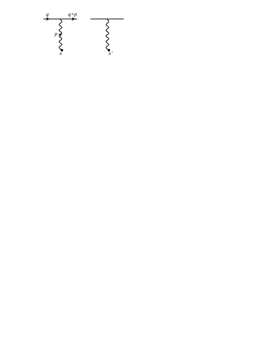
Figure 1: Feynman diagrams representing the disconnected part of correlation function [the second term in Eq. (2)]. Wavy lines denote the photon propagators, solid lines the massive particle. $q$ and $p$ are the particle 4-momentum and 4-momentum transfer, respectively.

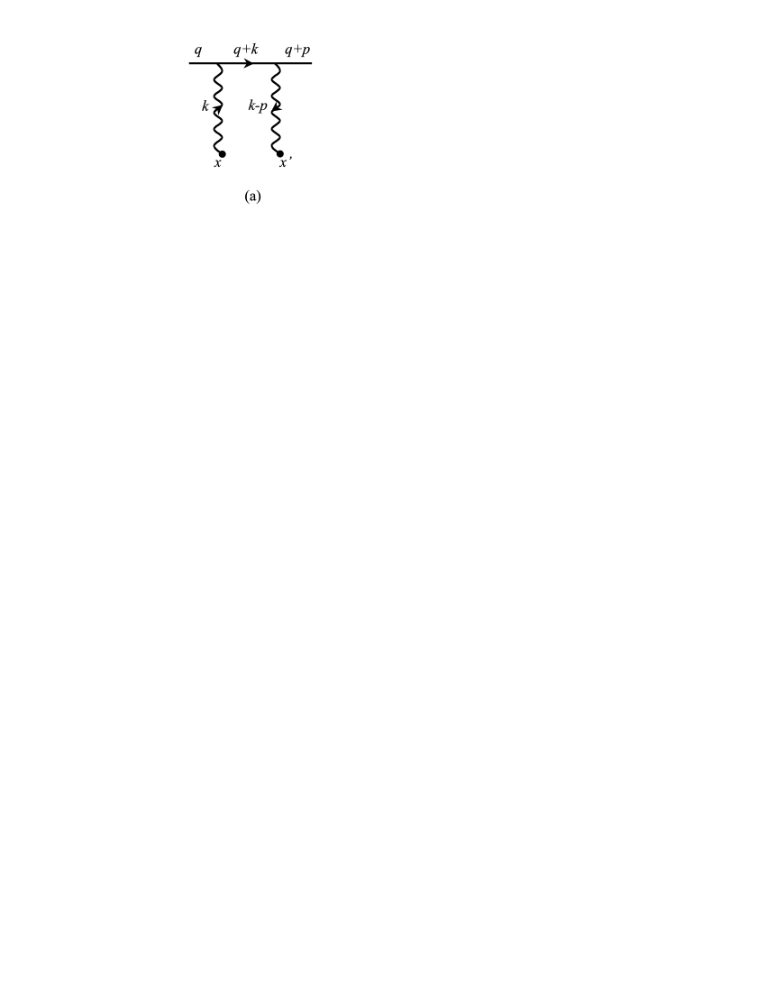
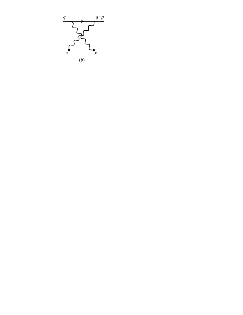
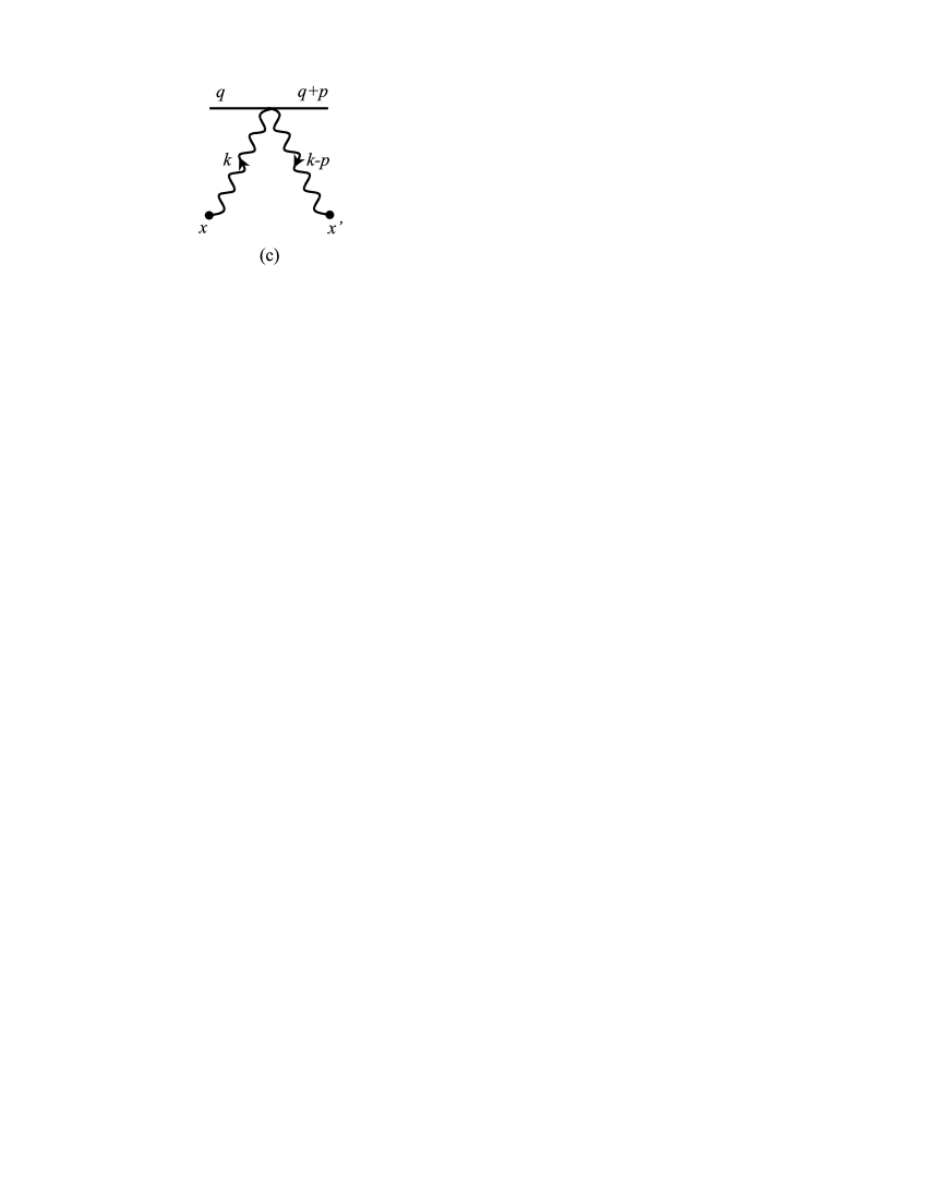
Figure 2: Feynman diagrams representing the connected part of correlation function [the first term in Eq. (2)].

where the Feynman weighting of the gauge condition is assumed. The tree diagrams generated by this action, which contribute to the right hand side of Eq. (2), are depicted in Figs. 1, 2.

To complete this section, let us define the power spectrum function of fluctuations. We are concerned with correlations in the values of the electromagnetic fields measured at two distinct time instants (spatial separation between the observation points, $|\bm{x}-\bm{x}^{\prime}|,$ is also kept arbitrary). Accordingly, fixing one of the time arguments, say, $t^{\prime},$ we define the power spectrum function as the Fourier transform of $C_{\mu\nu}(x,x^{\prime})$ with respect to $(t-t^{\prime})$

$$C_{\mu\nu}(\bm{x},\bm{x}^{\prime},t^{\prime},\omega)=\int\limits_{-\infty}^{+\infty}dtC_{\mu\nu}(x,x^{\prime})e^{i\omega(t-t^{\prime})}\,.$$ (6)

III Evaluation of the leading contribution

Evaluation of the low-frequency asymptotic of the correlation function proceeds in two steps. First, we will prove in Sec. III.1 that the low-frequency asymptotic of the connected part of $C_{\mu\nu}$ [the first term in Eq. (2)] is logarithmic. The contribution of the disconnected part will be calculated in Sec. III.2. It will be shown that this contribution exhibits an inverse frequency dependence, and thus dominates in the low-frequency limit.

III.1 Low-frequency asymptotic of the connected part of correlation function

Before going into detailed calculations, let us first exclude the diagrams in Fig. 2, which do not contain the $\hbar^{0}$ contribution. It is not difficult to see that these are the diagrams without internal matter lines, i.e. 2(c) in the present case. Indeed, this diagram is proportional to the integral

$$\int d^{4}k\frac{e^{ik(x-x^{\prime})}}{k^{2}(k-p)^{2}}\ ,$$

which does not involve the particle mass at all. Taking into account that each external matter line gives rise to the factor $(2\epsilon_{\bm{q}})^{-1/2},$ where $\epsilon_{\bm{q}}=\sqrt{m^{2}+\bm{q}^{2}}\approx m\,,$ we see that the contribution of diagram 2(c) is proportional to $1/m.$ Hence, on dimensional grounds, this diagram is proportional to $\hbar.$

The contribution of diagrams 2(a), 2(b) has the form

$$B_{\mu\nu} = I_{\mu\nu}(x,x^{\prime})+I_{\mu\nu}(x^{\prime},x)\,,$$

$$I_{\mu\nu}(x,x^{\prime}) = ie^{2}\iint d^{4}zd^{4}z^{\prime}D^{0}(x,z)\left[\phi_{0}^{*}(z)\stackrel{{\scriptstyle\leftrightarrow}}{{\partial_{\mu}}}D(z,z^{\prime})\stackrel{{\scriptstyle\leftrightarrow}}{{\partial_{\nu}^{\,\prime}}}\phi_{0}(z^{\prime})\right]D^{0}(z^{\prime},x^{\prime})\,,$$ (7)

where

$$\varphi\stackrel{{\scriptstyle\leftrightarrow}}{{\partial_{\mu}}}\psi = \varphi\partial_{\mu}\psi-\psi\partial_{\mu}\varphi\,,$$

$$D(x,y) = \int\frac{d^{4}k}{(2\pi)^{4}}\frac{e^{-ik(x-y)}}{m^{2}-k^{2}-i0}\,,$$

$$D^{0} \equiv D|_{m=0}\,,$$ (8)

and $\phi_{0}$ is the given particle state. Introducing the Fourier transform of $I_{\mu\nu}(x,x^{\prime})$

$$\tilde{I}_{\mu\nu}(\bm{x},\bm{x}^{\prime},t^{\prime},\omega)=\int\limits_{-\infty}^{+\infty}dtI_{\mu\nu}(x,x^{\prime})e^{i\omega(t-t^{\prime})}\,,$$

and going over to the momentum space, one finds

$$\tilde{I}_{\mu\nu}(\bm{x},\bm{x}^{\prime},t^{\prime},\omega) = e^{2}\iint\frac{d^{3}\bm{q}}{(2\pi)^{3}}\frac{d^{3}\bm{p}}{(2\pi)^{3}}\frac{a^{*}(\bm{q})a(\bm{q}+\bm{p})}{\sqrt{2\epsilon_{\bm{q}}2\epsilon_{{\bm{q}}+\bm{p}}}}e^{-ip^{0}(t^{\prime}-t_{0})+i\bm{p}\bm{x}^{\prime}}\tilde{J}_{\mu\nu}(p,q,\bm{x}-\bm{x}^{\prime},\omega)\,,$$ (9)

$$p^{0} = \epsilon_{\bm{q}+\bm{p}}-\epsilon_{\bm{q}}\,,$$

where

$$\tilde{J}_{\mu\nu}(p,q,\bm{x}-\bm{x}^{\prime},\omega)= -i\int\frac{d^{3}\bm{k}}{(2\pi)^{3}}e^{i\bm{k}(\bm{x}-\bm{x}^{\prime})}(2q_{\mu}+k_{\mu})(2q_{\nu}+k_{\nu}+p_{\nu})$$ (10)

$$\times\left.D^{0}(k)D(q+k)D^{0}(k-p)\right|_{k^{0}=\omega}\,.$$

Here $q_{\mu}$ is the particle 4-momentum, and $a(\bm{q})$ its momentum wave function at some time instant $t_{0}.$ The function $a(\bm{q})$ is normalized by

$$\int\frac{d^{3}\bm{q}}{(2\pi)^{3}}|a(\bm{q})|^{2}=1\,,$$ (11)

and is generally of the form

$$a(\bm{q})=b(\bm{q})e^{-i\bm{q}\bm{x}_{0}}\,,$$ (12)

where $\bm{x}_{0}$ is the particle mean position, and $b(\bm{q})$ describes the momentum space profile of the particle wave packet.

Let us now show that the low-frequency asymptotic of $\tilde{J}_{\mu\nu}$ is logarithmic. We note, first of all, that in the long-range limit, the 4-momenta $k_{\mu},p_{\mu}$ in the vertex factors can be neglected in comparison with $q_{\mu},$ because the leading contribution comes from integration over small $k_{\mu}.$ By the same reason, the factor $\exp\{i\bm{k}(\bm{x}-\bm{x}^{\prime})\}$ can be set equal to unity. Next, introducing the Schwinger parameterization of the propagators, we rewrite $\tilde{J}_{\mu\nu}$ as

$$\tilde{J}_{\mu\nu}(p,q,\omega)=4q_{\mu}q_{\nu}\int\frac{d^{3}\bm{k}}{(2\pi)^{3}}\exp\left\{i\left(x[\omega^{2}-\bm{k}^{2}]+y[\omega^{2}-\bm{k}^{2}+2m\omega-2(\bm{k}\bm{q})]\right.\right.$$

$$\left.\left.+z[(\omega-p^{0})^{2}-(\bm{k}-\bm{p})^{2}]\right)\right\}=\frac{q_{\mu}q_{\nu}}{2\pi^{3}}\iiint_{0}^{\infty}dxdydz\left(\frac{\pi e^{-i\pi/2}}{x+y+z}\right)^{3/2}\exp\left\{i\frac{(y\bm{q}-z\bm{p})^{2}}{x+y+z}\right\}$$

$$\times\exp\left\{i\left(x\omega^{2}+y[\omega^{2}+2m\omega]+z[(\omega-p^{0})^{2}-\bm{p}^{2}]\right)\right\}\,.$$

Changing the integration variables $y\to xy,$ $z\to xz,$ and integrating over $x$ gives

$$\tilde{J}_{\mu\nu}(p,q,\omega)=\frac{q_{\mu}q_{\nu}}{4\pi}\iint_{0}^{\infty}dydz\left\{(y\bm{q}-z\bm{p})^{2}\right.$$

$$\left.+(1+y+z)\left(\omega^{2}+y[\omega^{2}+2m\omega]+z[(\omega-p^{0})^{2}-\bm{p}^{2}]\right)\right\}^{-3/2}\,.$$

The singularity of the latter integral at $\omega=0$ comes from integration over small $y,z,$ therefore, it is the same as the singularity of the integral

$$\tilde{J}^{\prime}_{\mu\nu}(p,q,\omega)$$

$$=\frac{q_{\mu}q_{\nu}}{4\pi}\iint_{0}^{\infty}dydz\left\{y^{2}\bm{q}^{2}-2yz(\bm{q}\bm{p})+\omega^{2}+y[\omega^{2}+2m\omega]+z[(\omega-p^{0})^{2}-\bm{p}^{2}]\right\}^{-3/2}$$

$$=\frac{q_{\mu}q_{\nu}}{2\pi}\int_{0}^{\infty}\frac{dy}{(\omega-p^{0})^{2}-\bm{p}^{2}-2y(\bm{q}\bm{p})}\left\{y^{2}\bm{q}^{2}+\omega^{2}+y[\omega^{2}+2m\omega]\right\}^{-1/2}$$

$$=\frac{q_{\mu}q_{\nu}}{2\pi}\int_{0}^{\infty}\frac{dy}{(\omega-p^{0})^{2}-\bm{p}^{2}-2\omega y(\bm{q}\bm{p})}\left\{y^{2}\bm{q}^{2}+1+y[\omega+2m]\right\}^{-1/2}\,.$$

After the transformations performed, the singularity of the last integral for $\omega\to 0$ reappears at $y\to\infty,$ and hence, it coincides with the singularity of the integral

$$\tilde{J}^{\prime\prime}_{\mu\nu}(p,q,\omega)=\frac{q_{\mu}q_{\nu}}{2\pi|\bm{q}|}\int^{\infty}\frac{dy}{y}\frac{1}{(\omega-p^{0})^{2}-\bm{p}^{2}-2\omega y(\bm{q}\bm{p})}$$

$$=\frac{q_{\mu}q_{\nu}}{2\pi|\bm{q}|\{(\omega-p^{0})^{2}-\bm{p}^{2}\}}\ln\left.\frac{y}{(\omega-p^{0})^{2}-\bm{p}^{2}-2\omega y(\bm{q}\bm{p})}\right|^{\infty}\sim\frac{q_{\mu}q_{\nu}}{2\pi|\bm{q}|p^{2}}\ln\frac{1}{\omega}\,.$$ (13)

It is not difficult to verify that the obtained expression agrees with the results of Sec. III A of Ref. kazakov . Thus, we have proved that the connected part of the correlation function diverges for $\omega\to 0$ only logarithmically.

III.2 Low-frequency asymptotic of the disconnected part of correlation function

Let us turn to the disconnected part of the correlation function. To find its Fourier transform, we have to evaluate the integral

$$\int\limits_{-\infty}^{+\infty}dt\,\langle{\rm in}|A_{\mu}(x)|{\rm in}\rangle e^{i\omega(t-t^{\prime})}=\frac{eq_{\mu}}{\epsilon_{\bm{q}}}e^{-i\omega t^{\prime}}\tilde{I}(\bm{r},\omega)\,,$$ (14)

where

$$\tilde{I}(\bm{r},\omega) = \int\limits_{-\infty}^{+\infty}dt\left\{e^{i\omega t}\iint\frac{d^{3}\bm{q}}{(2\pi)^{3}}\frac{d^{3}\bm{p}}{(2\pi)^{3}}\frac{e^{i\bm{p}\bm{r}}}{\bm{p}^{2}}e^{-ip^{0}(t-t_{0})}b^{*}(\bm{q})b(\bm{q}+\bm{p})\right\}\,,\quad\bm{r}=\bm{x}-\bm{x}_{0}\,.$$

To the leading order of the long-range expansion, $b(\bm{q}+\bm{p})$ can be substituted here by $b(\bm{q}).$ Using also

$$p^{0}\approx\frac{(\bm{p}+\bm{q})^{2}}{2m}-\frac{\bm{q}^{2}}{2m}$$

gives

$$\tilde{I}(\bm{r},\omega)=2\pi e^{i\omega t_{0}}\iint\frac{d^{3}\bm{q}}{(2\pi)^{3}}\frac{d^{3}\bm{p}}{(2\pi)^{3}}\delta\left(\omega-\frac{\bm{p}^{2}+2\bm{pq}}{2m}\right)\frac{e^{i\bm{p}\bm{r}}}{\bm{p}^{2}}|b(\bm{q})|^{2}\,.$$

The function $b(\bm{q})$ will be assumed to possess the symmetry of the external field. Thus, in the presence of a homogeneous external electric field, the function $b(\bm{q})$ is axially-symmetric; taking $z$ axis in the direction of the field, one has $b(\bm{q})=b(q_{\bot},q_{z}),$ where $q_{\bot}=\sqrt{\bm{q}^{2}-q^{2}_{z}}$ is the transverse component of the particle momentum. In this case, $\tilde{I}$ is a function of $\zeta=r_{z}$ and $\rho=\sqrt{\bm{r}^{2}-\zeta^{2}},$ $\tilde{I}(\bm{r},\omega)=\tilde{I}(\rho,\zeta,\omega),$ and hence, averaging over transverse directions, one can write

$$\tilde{I}(\rho,\zeta,\omega) = 2\pi e^{i\omega t_{0}}\iint\frac{d^{3}\bm{q}}{(2\pi)^{3}}\frac{d^{3}\bm{p}}{(2\pi)^{3}}\delta\left(\omega-\frac{\bm{p}^{2}+2\bm{pq}}{2m}\right)\frac{J_{0}(|\bm{p}|\rho\sin\phi)}{\bm{p}^{2}}e^{i|\bm{p}|\zeta\cos\phi}|b(q_{\bot},q_{z})|^{2}\,,$$

where $\phi$ is the angle between $\bm{p}$ and $z$ axis, and $J_{0}$ is the Bessel function. To evaluate the $\bm{p}$ integral it is convenient to introduce a spherical coordinate system, with the polar axis pointing in the direction of the vector $\bm{q}.$ Let the azimuthal and polar angles of $\bm{p}$ in this system be denoted by $\varphi,\theta,$ and those of $z$ axis by $\varphi^{\prime},\theta^{\prime},$ respectively. Then

$$\cos\phi=\sin\theta\sin\theta^{\prime}\cos(\varphi-\varphi^{\prime})+\cos\theta\cos\theta^{\prime}\,,$$

and

$$\tilde{I}(\rho,\zeta,\omega) = \frac{me^{i\omega t_{0}}}{(2\pi)^{2}}\int\frac{d^{3}\bm{q}}{(2\pi)^{3}}|\beta(q_{\bot},q_{z})|^{2}\int\limits_{0}^{\pi}d\theta\sin\theta\int\limits_{0}^{2\pi}d\varphi\frac{J_{0}(u\rho\sin\phi)e^{iu\zeta\cos\phi}}{\sqrt{\bm{q}^{2}\cos^{2}\theta+2m\omega}}\,,$$ (15)

$$u = -|\bm{q}|\cos\theta+\sqrt{\bm{q}^{2}\cos^{2}\theta+2m\omega}\,,$$

where it is assumed that $\omega>0.$ Since the integrand in this formula depends on the difference $\varphi-\varphi^{\prime},$ the result of integration over $\varphi$ is independent of $\varphi^{\prime}.$ Setting the latter equal to zero, and taking $\phi$ as the integration variable yields

$$\mathcal{I}\equiv\int\limits_{0}^{2\pi}d\varphi J_{0}(u\rho\sin\phi)e^{iu\zeta\cos\phi}=2\int\limits_{\theta-\theta^{\prime}}^{\theta+\theta^{\prime}}d\phi\frac{\sin\phi\,J_{0}(u\rho\sin\phi)e^{iu\zeta\cos\phi}}{\sqrt{[\cos\phi-\cos(\theta+\theta^{\prime})][\cos(\theta-\theta^{\prime})-\cos\phi]}}\,.$$ (16)

It is seen from Eq. (III.2) that the singularity at $\omega=0$ comes from integration over $\theta\approx\pi/2.$ Without changing the singular contribution, therefore, one can set $\theta=\pi/2$ in the integral (16), which after simple transformations takes the form

$$\mathcal{I}=4\int\limits_{0}^{1}dv\frac{J_{0}\left(u\rho\sqrt{1-\sin^{2}\theta^{\prime}v^{2}}\right)\cos\left(uv\zeta\sin\theta^{\prime}\right)}{\sqrt{1-v^{2}}}\,.$$ (17)

In the long-range limit, the argument of the Bessel function is large, so one can use the asymptotic formula

$$J_{0}(z)=\sqrt{\frac{2}{\pi z}}\cos\left(z-\frac{\pi}{4}\right)\,.$$

Thus, the above integral involves rapidly oscillating trigonometric functions, and the leading contribution comes from integration around the point of stationary phase of the integrand. Assuming $\zeta>0,$ and decomposing the product of cosines into a sum, one sees that the range of integration contains one such point, if $\zeta<r\sin\theta^{\prime},$ namely

$$v_{0}=\frac{\zeta}{r\sin\theta^{\prime}}\,,$$

and hence

$$\mathcal{I} \approx 2\sqrt{\frac{2}{\pi}}\ {\rm Re}\int\limits_{0}^{1}dv\frac{\displaystyle\exp\left\{i\left(u\rho\sqrt{1-\sin^{2}\theta^{\prime}v^{2}}+uv\zeta\sin\theta^{\prime}-\frac{\pi}{4}\right)\right\}}{\sqrt{(1-v^{2})u\rho\sqrt{1-\sin^{2}\theta^{\prime}v^{2}}}}$$ (18)

$$\approx 2\sqrt{\frac{2}{\pi}}\ {\rm Re}\int\limits_{0}^{1}dv\frac{\displaystyle\exp\left\{i\left(ur-\frac{ur^{3}}{2\rho^{2}}\sin^{2}\theta^{\prime}(v-v_{0})^{2}-\frac{\pi}{4}\right)\right\}}{\sqrt{(1-v^{2})u\rho\sqrt{1-\sin^{2}\theta^{\prime}v^{2}}}}$$

$$\approx 2\sqrt{\frac{2}{\pi}}\ {\rm Re}\frac{\displaystyle\exp\left\{i\left(ur-\frac{\pi}{2}\right)\right\}}{\sqrt{(1-v_{0}^{2})u\rho\sqrt{1-\sin^{2}\theta^{\prime}v_{0}^{2}}}}\sqrt{\frac{2\pi\rho^{2}}{ur^{3}\sin^{2}\theta^{\prime}}}=\frac{4\sin(ur)}{\displaystyle ur\sqrt{\sin^{2}\theta^{\prime}-\frac{\zeta^{2}}{r^{2}}}}\,.$$

Substituting this in Eq. (III.2), introducing a new spherical system of coordinates, with the polar axis in $z$ direction, and noting that $\theta^{\prime}$ is the polar angle of the vector $\bm{q}$ gives

$$\tilde{I}(\rho,\zeta,\omega) = \frac{me^{i\omega t_{0}}}{4\pi^{4}r}\int\limits_{\arcsin\zeta/r}^{\pi-\arcsin\zeta/r}\frac{d\theta^{\prime}\sin\theta^{\prime}}{\displaystyle\sqrt{\sin^{2}\theta^{\prime}-\frac{\zeta^{2}}{r^{2}}}}\int\limits_{0}^{\infty}dq\,q^{2}|\beta(q,\theta^{\prime})|^{2}\int\limits_{0}^{\pi}d\theta\frac{\sin\theta\sin(ur)}{\displaystyle u\sqrt{q^{2}\cos^{2}\theta+2m\omega}}\,,$$

$$u = -q\cos\theta+\sqrt{q^{2}\cos^{2}\theta+2m\omega}\,,\quad\beta(q,\theta^{\prime})\equiv b(q\sin\theta^{\prime},q\cos\theta^{\prime})\,,$$

or, taking $u$ as the integration variable,

$$\tilde{I}(\rho,\zeta,\omega) = \frac{me^{i\omega t_{0}}}{4\pi^{4}r}\int\limits_{\arcsin\zeta/r}^{\pi-\arcsin\zeta/r}\frac{d\theta^{\prime}\sin\theta^{\prime}}{\displaystyle\sqrt{\sin^{2}\theta^{\prime}-\frac{\zeta^{2}}{r^{2}}}}\int\limits_{0}^{\infty}dq\,q|\beta(q,\theta^{\prime})|^{2}\int\limits_{\sqrt{\bm{q}^{2}+2m\omega}-|\bm{q}|}^{\sqrt{\bm{q}^{2}+2m\omega}+|\bm{q}|}du\frac{\sin(ur)}{u^{2}}\,.$$ (19)

To further transform this integral, it is convenient to define a function $\Gamma(q,\theta,\omega)$ according to

$$\Gamma(q,\theta)=\frac{1}{2\pi^{2}}\int\limits_{q}^{+\infty}dw\,w|\beta(w,\theta)|^{2}\,.$$ (20)

Then integrating by parts, and taking into account that $\Gamma(q,\theta,\omega)\to 0$ for $q\to\infty,$ brings Eq. (19) to the form

$$\tilde{I}(\rho,\zeta,\omega) = \frac{me^{i\omega t_{0}}}{2\pi^{2}r}\int\limits_{\arcsin\zeta/r}^{\pi-\arcsin\zeta/r}\frac{d\theta\sin\theta}{\displaystyle\sqrt{\sin^{2}\theta-\frac{\zeta^{2}}{r^{2}}}}\int\limits_{0}^{+\infty}dq\frac{\Gamma(q,\theta)}{\sqrt{q^{2}+2m\omega}}$$ (21)

$$\times\biggl{\{}\left.\frac{\sin(ur)}{u}\right|_{u=\sqrt{q^{2}+2m\omega}+q}+\left.\frac{\sin(ur)}{u}\right|_{u=\sqrt{q^{2}+2m\omega}-q}\biggr{\}}\,.$$

Finally, integrating $\tilde{I}$ by parts once more, we find

$$\tilde{I}(\rho,\zeta,\omega) = \frac{e^{i\omega t_{0}}}{2\pi^{2}r\omega}\int\limits_{\arcsin\zeta/r}^{\pi-\arcsin\zeta/r}\frac{d\theta\sin\theta}{\displaystyle\sqrt{\sin^{2}\theta-\frac{\zeta^{2}}{r^{2}}}}\int\limits_{0}^{+\infty}dq$$ (22)

$$\times\sin\left(r\sqrt{q^{2}+2m\omega}\right)\left\{2\Gamma\cos(qr)+\frac{1}{r}\frac{\partial\Gamma}{\partial q}\sin(qr)\right\}\,.$$

This expression considerably simplifies in the practically important case of low $\omega$ and large $r.$ Namely, if $\omega$ is such that

$$\omega\ll\frac{\tilde{D}}{mr}\equiv\omega_{0}\,,$$ (23)

and also

$$r\tilde{D}\gg 1$$ (24)

(and therefore, $\omega\ll\tilde{D}^{2}/m$), then the first term in $\tilde{I}$ turns out to be exponentially small ($\sim e^{-r\tilde{D}}$) because of the oscillating product of trigonometric functions. Replacing $\sin^{2}(qr)$ by its average value (1/2) in the rest of $\tilde{I}$ gives

$$\tilde{I}(\rho,\zeta,\omega) = \frac{e^{i\omega t_{0}}}{4\pi^{2}r^{2}\omega}\int\limits_{\arcsin\zeta/r}^{\pi-\arcsin\zeta/r}\frac{d\theta\sin\theta}{\displaystyle\sqrt{\sin^{2}\theta-\frac{\zeta^{2}}{r^{2}}}}\int\limits_{0}^{+\infty}dq\frac{\partial\Gamma}{\partial q}=-\frac{e^{i\omega t_{0}}}{4\pi^{2}r^{2}\omega}\int\limits_{\arcsin\zeta/r}^{\pi-\arcsin\zeta/r}\frac{d\theta\sin\theta\Gamma(0,\theta)}{\displaystyle\sqrt{\sin^{2}\theta-\frac{\zeta^{2}}{r^{2}}}}\,,$$

or,

$$\tilde{I}(\rho,\zeta,\omega)=-\frac{e^{i\omega t_{0}}}{8\pi^{4}r^{2}\omega}\int\limits_{\chi}^{\pi-\chi}\frac{d\theta\sin\theta}{\displaystyle\sqrt{\sin^{2}\theta-\sin^{2}\chi}}\int\limits_{0}^{+\infty}dq\,q|\beta(q,\theta)|^{2}\,,$$ (25)

where $\chi$ is the angle between the vector $\bm{r}$ and $x,y$ plane, $\sin\chi=\zeta/r.$

In the case of a spherically symmetric wave function, $\beta(q,\theta)=\beta(q),$ integration over $\theta$ in Eq. (25) yields the expression derived in Ref. kazakov

$$\tilde{I}(\rho,\zeta,\omega)=-\frac{e^{i\omega t_{0}}}{8\pi^{3}r^{2}\omega}\int\limits_{0}^{+\infty}dq\,q|\beta(q)|^{2}\,.$$ (26)

It has been assumed in the course of derivation of Eq. (25) that $\omega>0,$ $\zeta>0.$ It is not difficult to verify that in the general case, $\tilde{I}(\rho,\zeta,\omega)=e^{i(\omega-|\omega|)t_{0}}\tilde{I}(\rho,|\zeta|,|\omega|).$

Substituting the obtained expression into the defining equations (14), (2), (6), we thus obtain the following expression for the low-frequency asymptotic of the correlation function

$$C_{00}(\rho,\zeta,r^{\prime},\omega) = e^{i\omega(t_{0}-t^{\prime})}\frac{e^{2}}{32\pi^{5}r^{2}r^{\prime}|\omega|}\int\limits_{|\chi|}^{\pi-|\chi|}\frac{d\theta\sin\theta}{\displaystyle\sqrt{\sin^{2}\theta-\sin^{2}\chi}}\int\limits_{0}^{+\infty}dq\,q|\beta(q,\theta)|^{2}\,,$$ (27)

all other components of the correlation function being suppressed by the factor $|\bm{q}|/m.$

In applications to microelectronics, $\omega$ varies from $10^{-6}{\rm Hz}$ to $10^{6}\,{\rm Hz},$ the relevant distances $r$ are usually $10^{-5}\,{\rm cm}$ to $10^{-2}\,{\rm cm},$ $\tilde{D}\sim\hbar/d,$ where $d\approx 10^{-8}\,{\rm cm}$ is the lattice spacing, and $m$ is the effective electron mass, $m\approx 10^{-27}\,{\rm g},$ hence, $\omega_{0}\approx 10^{10}\,{\rm Hz},$ so the conditions $r\gg d,$ $\omega\ll\omega_{0}$ are always well-satisfied.

In connection with the application of the obtained results to solids, it should be stressed that they refer to long-living free-evolving electron states. At the same time, because of collisions of electrons with phonons, impurities, and with each other, their evolution in a crystal usually cannot be considered free. It is important, however, that in view of smallness of the electron mass in comparison with the atomic masses, the electron collisions with phonons and impurities may often be considered elastic. Such collisions do not change the electron energy, and therefore they do not influence time evolution of the electron wave function. As to the electron-electron collisions, they do change the energy of electrons. However, the electron component in solids is practically always degenerate, and hence, only electrons with energies near the Fermi surface are actually scattered. Therefore, the above results concerning dispersion of the electromagnetic field fluctuations remain essentially the same despite the electron collisions, provided that they are applied to electrons far from the Fermi surface, and expressed in terms of the electron density matrix, rather than the wave function. Denoting the diagonal elements of the momentum space density matrix of electrons by $\varrho(q,\theta),$ Eq. (27) thus takes the form

$$C_{00}(\rho,\zeta,r^{\prime},\omega) = e^{i\omega(t_{0}-t^{\prime})}\frac{e^{2}}{32\pi^{5}r^{2}r^{\prime}|\omega|}\int\limits_{|\chi|}^{\pi-|\chi|}\frac{d\theta\sin\theta}{\displaystyle\sqrt{\sin^{2}\theta-\sin^{2}\chi}}\int\limits_{0}^{+\infty}dq\,q\varrho(q,\theta)\,.$$ (28)

The power spectrum of the noise produced by uncorrelated electrons in a sample can be found by integrating Eq. (28) with respect to $\bm{x}_{0}$ over the sample volume. If the time instants $t_{0}$ are distributed uniformly (which is natural to expect), then the value of the total noise spectrum function, $C^{\rm tot}_{00},$ remains at the level of the individual contribution (28) independently of the number of electrons in the sample, because of cancellation of the alternating phase factors $e^{i\omega t_{0}}$.

IV The noise induced by external electric field

According to the property 3) of observed flicker noise, mentioned in the introduction, power spectrum of the noise induced by external electric field is proportional to $\bm{E}^{2},$ at least for sufficiently small values of the field strength $\bm{E}.$ If the density matrix $\varrho$ were analytic with respect to $\bm{E},$ then the scalar function $C^{\rm tot}_{00}(\bm{E})-C^{\rm tot}_{00}(0)\equiv\Delta C^{\rm tot}_{00}(\bm{E})$ would expand in even powers of $\bm{E},$ and therefore, the leading term would be quadratic in the field strength, as required. However, $\varrho$ is not generally analytic in $\bm{E},$ and therefore, the expansion of $\Delta C^{\rm tot}_{00}(\bm{E})$ might contain, e.g., a term proportional to $|\bm{E}|,$ in contradiction with the experiment. Thus, our primary concern below will be the weak field asymptotic of the power spectrum given by Eq. (28). There is actually a simple and general reason why the right hand side of this equation should be quadratic in $\bm{E}$ despite possible non-analyticity of the density matrix $\varrho.$ This matrix is a functional of the equilibrium density matrix, $\varrho_{0},$ and of the field strength. As was mentioned in the preceding section, the electron states responsible for the $1/\omega$ behavior of the correlation function are those with energies far from the Fermi surface. For such states, the function $\varrho$ is a constant inversely proportional to the electron density, in particular, it is independent of parameters characterizing the Fermi surface, such as Fermi energy or momentum. Therefore, on dimensional grounds, the integral on the right of Eq. (28) should be proportional to the square of a characteristic momentum built from the field strength. The only such momentum is $e|\bm{E}|\tau,$ where $\tau$ is some time parameter characterizing electron kinetics, and hence, $\Delta C^{\rm tot}_{00}\sim\bm{E}^{2}\,.$ This reasoning will be illustrated below using the simplest kinetic model with the relaxation-type collision term, which admits full theoretic investigation.

In the presence of a constant homogeneous electric field, the model kinetic equation reads

$$eE\frac{\partial\varrho}{\partial q_{z}}=-\frac{\varrho-\varrho_{0}}{\tau}\,,$$ (29)

where $z$ axis is chosen in the direction of $\bm{E}$ ($E_{z}=|\bm{E}|\equiv E$), $\tau$ is the relaxation time, and $\varepsilon$ the electron energy. Since Eq. (28) was obtained for a free electron, we assume that the band structure in the given solid is parabolic, $\varepsilon=\bm{q}^{2}/2m^{*},$ where $m^{*}$ is the effective electron mass. According to Eq. (11), the function $\varrho$ is normalized by

$$\int\frac{d^{3}\bm{q}}{(2\pi)^{3}}\varrho(\varepsilon)=1\,.$$

If the function $\varrho_{0}$ satisfies this condition, then the normalized solution of the kinetic equation (29) has the form

$$\varrho=\frac{e^{q_{z}/q_{0}}}{q_{0}}\int\limits_{q_{z}}^{\infty}d\xi e^{-\xi/q_{0}}\varrho_{0}(\varepsilon^{\prime})\,,\quad\varepsilon^{\prime}=\frac{1}{2m^{*}}(q^{2}_{\bot}+\xi^{2})\,,\quad q_{0}=|e|E\tau\,.$$ (30)

Thus, in order to find the quantity $C_{00},$ we have to calculate the following integral

$$K=\int\limits_{\chi}^{\pi-\chi}\frac{d\theta\sin\theta}{\displaystyle\sqrt{\sin^{2}\theta-\sin^{2}\chi}}\int\limits_{0}^{+\infty}dq\,q\frac{e^{q\cos\theta/q_{0}}}{q_{0}}\int\limits_{q\cos\theta}^{\infty}d\xi e^{-\xi/q_{0}}\varrho_{0}(\varepsilon^{\prime})\,,\quad\varepsilon^{\prime}=\frac{1}{2m^{*}}(q^{2}\sin^{2}\theta+\xi^{2})\,.$$

Changing the integration variables $q,\theta\to\zeta,\eta$ according to

$$\cos\theta=\frac{\zeta\cos\chi}{\sqrt{\zeta^{2}+\eta^{2}}}\,,\quad q^{2}=\zeta^{2}+\eta^{2}$$

brings this integral to the form

$$K=\iint\limits_{-\infty}^{+\infty}d\zeta d\eta\frac{e^{\zeta\cos\chi/q_{0}}}{2q_{0}}\int\limits_{\zeta\cos\chi}^{\infty}d\xi e^{-\xi/q_{0}}\varrho_{0}(\varepsilon^{\prime\prime})\,,\quad\varepsilon^{\prime\prime}=\frac{1}{2m^{*}}(\eta^{2}+\zeta^{2}\sin^{2}\chi+\xi^{2})\,.$$

Integrating by parts with respect to $\zeta$ yields

$$K=\frac{1}{2}\iint\limits_{-\infty}^{+\infty}d\zeta d\eta\varrho_{0}\left(\frac{\zeta^{2}+\eta^{2}}{2m^{*}}\right)-\frac{\sin^{2}\chi}{2m^{*}\cos\chi}\iint\limits_{-\infty}^{+\infty}d\zeta d\eta~{}\zeta e^{\zeta\cos\chi/q_{0}}\int\limits_{\zeta\cos\chi}^{\infty}d\xi e^{-\xi/q_{0}}\frac{d\varrho_{0}}{d\varepsilon}(\varepsilon^{\prime\prime})\,.$$

The first term in this expression represents the value of the quantity $K$ in the absence of the external field. Therefore, performing a shift $\xi\to\xi+\zeta\cos\chi,$ and then $\zeta\to\zeta-\xi\cos\chi$ in the remaining integral, we find the part induced by the electric field

$$\Delta K=\frac{\sin^{2}\chi}{2m^{*}}\iint\limits_{-\infty}^{+\infty}d\zeta d\eta\int\limits_{0}^{\infty}d\xi~{}\xi e^{-\xi/q_{0}}\frac{d\varrho_{0}}{d\varepsilon}(\varepsilon^{\prime\prime\prime})\,,\quad\varepsilon^{\prime\prime\prime}=\frac{1}{2m^{*}}(\eta^{2}+\zeta^{2}+\xi^{2}\sin^{2}\chi)\,.$$

Going over to the polar coordinates in the $(\zeta,\eta)$ plane gives finally

$$\Delta K=\pi\sin^{2}\chi\int\limits_{0}^{\infty}d\xi~{}\xi e^{-\xi/q_{0}}\int\limits_{\xi^{2}\sin^{2}\chi/2m^{*}}^{+\infty}d\varepsilon\frac{d\varrho_{0}}{d\varepsilon}(\varepsilon)=-\pi\sin^{2}\chi\int\limits_{0}^{\infty}d\xi~{}\xi e^{-\xi/q_{0}}\varrho_{0}\left(\frac{\xi^{2}\sin^{2}\chi}{2m^{*}}\right)\,.$$

In the case of a degenerate electron system, the function $\varrho_{0}(\varepsilon)$ is nearly constant up to Fermi energy where it falls off to zero. For such a function, $\Delta K\sim q_{0}^{2},$ up to exponentially small terms, provided that $q_{0}$ is sufficiently small. Indeed, assuming $q_{0}\ll q_{F},$ where $q_{F}$ is the electron momentum at the Fermi surface, and neglecting terms of the order $e^{-q_{F}/q_{0}},$ one can substitute $\varrho_{0}\left(\frac{\xi^{2}\sin^{2}\chi}{2m^{*}}\right)$ by $\varrho_{0}(0)$ in the above integral to obtain

$$\Delta K=-\pi\sin^{2}\chi\varrho_{0}(0)\int\limits_{0}^{\infty}d\xi~{}\xi e^{-\xi/q_{0}}=-q_{0}^{2}\varrho_{0}(0)\pi\sin^{2}\chi\,.$$

Inserting this into Eq. (28), we arrive at the following expression for the power spectrum of the induced noise

$$\Delta C_{00} = -e^{i\omega(t_{0}-t^{\prime})}\frac{e^{2}q_{0}^{2}\varrho_{0}(0)\zeta^{2}}{32\pi^{4}r^{4}r^{\prime}|\omega|}\,.$$ (31)

Thus, $\Delta C_{00}\sim\bm{E}^{2},$ as was to be shown. It is important that the correction terms are of the order $\exp^{-q_{F}/q_{0}},$ and hence, from the practical point of view, the condition $q_{0}\ll q_{F}$ amounts to $q_{0}<q_{F}.$ This implies that the upper limit on the field strengths for which Eq. (31) is valid is well above all experimentally relevant values.

Let us compare this result with the power spectrum of quantum fluctuations in the absence of external field, obtained in Ref. kazakov , which in the present notation has the form

$$C_{00}(0)=e^{i\omega(t_{0}-t^{\prime})}\frac{e^{2}}{32\pi^{4}r^{2}r^{\prime}|\omega|}\int\limits_{0}^{+\infty}dq\,q\varrho_{0}(\varepsilon)\,.$$

By the order of magnitude,

$$\frac{\Delta C_{00}}{C_{00}(0)}\sim\frac{q^{2}_{0}\varrho_{0}(0)}{\int\limits_{0}^{+\infty}dq\,q\varrho_{0}}\sim q_{F}q^{2}_{0}\varrho_{0}(0)\sim\frac{q^{2}_{0}}{q^{2}_{F}}\,,$$

since $\varrho_{0}(0)\sim q^{-3}_{F}\,.$ Thus, in the model considered, the induced noise represents a relatively small correction.

In practice, one is interested in fluctuations of the voltage, $U,$ between two leads attached to a sample. Using the above results, it is not difficult to write down an expression for the voltage correlation function, $C_{\rm U}(\bm{x},\bm{x}^{\prime},\omega)$. We have

$$\langle\hat{U}(\bm{x},\bm{x}^{\prime},t)\rangle\langle\hat{U}(\bm{x},\bm{x}^{\prime},t^{\prime})\rangle = \langle\hat{A}_{0}(\bm{x},t)-\hat{A}_{0}(\bm{x}^{\prime},t)\rangle\langle\hat{A}_{0}(\bm{x},t^{\prime})-\hat{A}_{0}(\bm{x}^{\prime},t^{\prime})\rangle$$ (32)

$$= \langle\hat{A}_{0}(\bm{x},t)\rangle\langle\hat{A}_{0}(\bm{x},t^{\prime})\rangle+\langle\hat{A}_{0}(\bm{x}^{\prime},t)\rangle\langle\hat{A}_{0}(\bm{x}^{\prime},t^{\prime})\rangle$$

$$- \langle\hat{A}_{0}(\bm{x}^{\prime},t)\rangle\langle\hat{A}_{0}(\bm{x},t^{\prime})\rangle-\langle\hat{A}_{0}(\bm{x},t)\rangle\langle\hat{A}_{0}(\bm{x}^{\prime},t^{\prime})\rangle\,,$$

where $\langle\cdots\rangle$ denotes averaging over the given in state. Fourier transforming and applying Eq. (31) to each of the four terms in this expression, we obtain the power spectrum of the induced voltage fluctuation across the sample

$$\Delta C_{U} = -e^{i\omega(t_{0}-t^{\prime})}\frac{e^{2}q_{0}^{2}\varrho_{0}(0)}{32\pi^{4}|\omega|}\left(\frac{\zeta^{2}}{r^{5}}+\frac{\zeta^{\prime 2}}{r^{\prime 5}}-\frac{\zeta^{\prime 2}}{r^{\prime 4}r}-\frac{\zeta^{2}}{r^{4}r^{\prime}}\right)\,.$$ (33)

This equation represents an individual contribution of an electron to the electric potential fluctuation. As was mentioned at the end of Sec. III.2, because of the oscillating exponent $e^{i\omega t_{0}},$ the magnitude of the total noise remains at the level of the individual contribution independently of the number of electrons. Therefore, summing up all contributions amounts simply to averaging over $\bm{x}_{0}:$

$$\left|\Delta C_{U}^{\rm tot}\right|=\frac{e^{2}q_{0}^{2}\varrho_{0}(0)G}{32\pi^{4}|\omega|\Omega}\,,$$ (34)

where

$$G\equiv\int\limits_{\Omega}d^{3}\bm{x}_{0}\left(\frac{\zeta^{2}}{r^{5}}+\frac{\zeta^{\prime 2}}{r^{\prime 5}}-\frac{\zeta^{\prime 2}}{r^{\prime 4}r}-\frac{\zeta^{2}}{r^{4}r^{\prime}}\right)$$ (35)

is a dimensionless geometrical factor, and $\Omega$ is the sample volume.

It is convenient to express the right hand side of Eq. (34) through the number of electrons in the sample, $N,$ rather than the sample volume. Taking into account that for degenerate electrons, $\varrho_{0}(0)=2/n,$ where $n$ is the electron density (the factor $2$ accounts for two spin states), substituting $n=N/\Omega,$ $q_{0}=|e|E\tau,$ and restoring the ordinary units brings Eq. (34) to the form

$$\left|\Delta C_{U}^{\rm tot}\right|=\frac{e^{4}}{32\pi^{5}\hbar^{2}}\frac{E^{2}\tau^{2}G}{Nf}\,,$$ (36)

where $f=|\omega|/2\pi.$ Finally, if the voltage leads are aligned in $z$ direction, as is usually the case, Eq. (36) can be rewritten as

$$\left|\Delta C_{U}^{\rm tot}\right|=\frac{\alpha\bar{U}^{2}}{Nf}\,,\quad\alpha=\frac{e^{4}\tau^{2}G}{32\pi^{5}l^{2}\hbar^{2}}\,,$$ (37)

where $\bar{U}$ is the average voltage across the sample, and $l$ is the sample length in the direction of the electric field. In this form, it is similar to the well-known empirical Hooge law, except that $N$ in Eq. (37) is the total number of electrons in the sample, rather than the number of charge carriers. We see that the analog of the Hooge constant, $\alpha,$ depends on physical properties of the sample material as well as on the sample geometry.

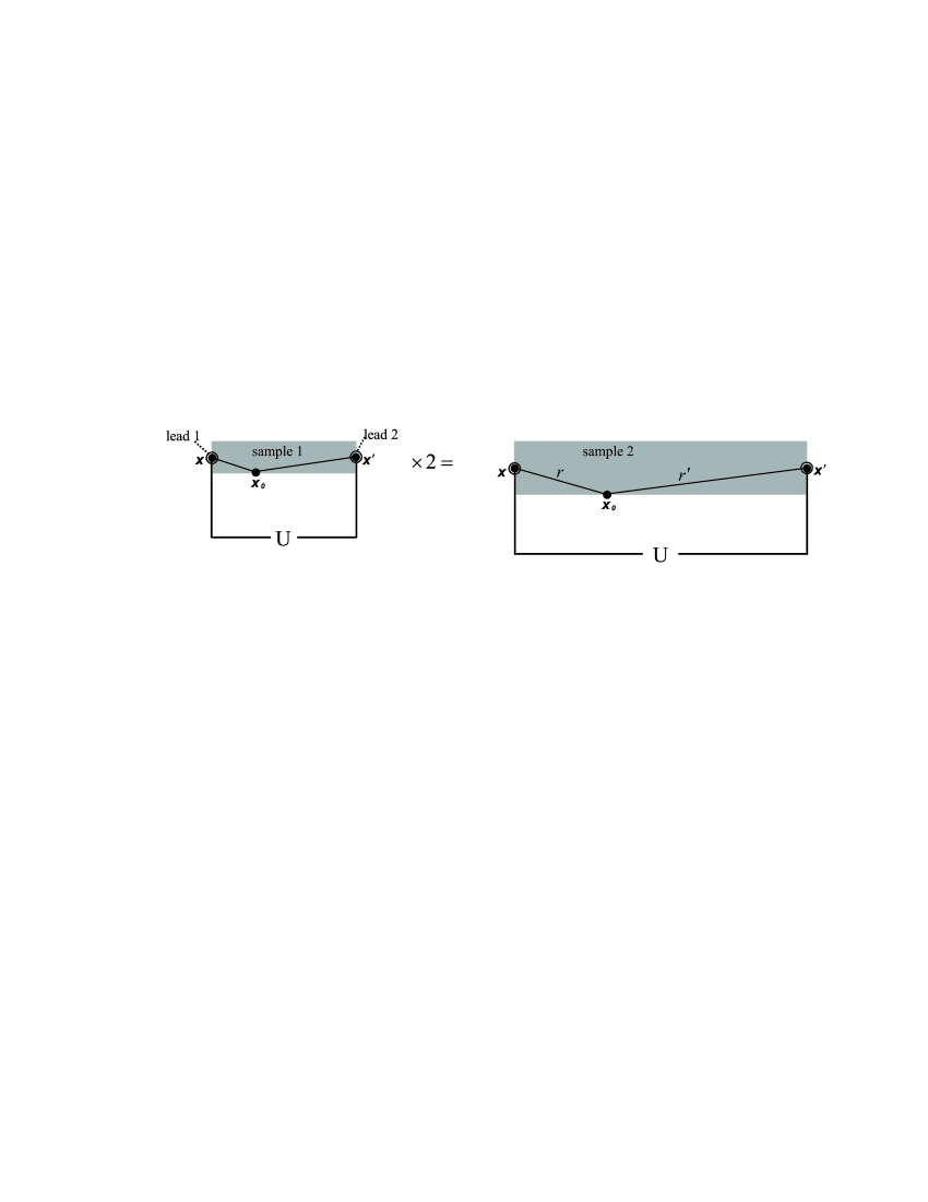
Figure 3: Voltage measurement in geometrically similar samples ($s=2$).

Let us discuss the role of the sample geometry in somewhat more detail. Consider two geometrically similar samples, and let $s$ be the ratio of their linear dimensions (see Fig. 3). It turns out that such samples are characterized by the same value of the $G$-factor. Indeed, since the voltage across the sample is usually measured via two leads attached to its surface, the radius-vectors of the leads drawn from the center of similitude scale by the same factor $s,$ and therefore,

$$\int\limits_{\Omega_{2}}d^{3}\bm{x}_{0}\frac{\zeta^{2}}{r^{4}r^{\prime}} = \int\limits_{s^{3}\Omega_{1}}d^{3}\bm{x}_{0}\frac{(sz-z_{0})^{2}}{|s\bm{x}-\bm{x}_{0}|^{4}|s\bm{x}^{\prime}-\bm{x}_{0}|}=\int\limits_{\Omega_{1}}s^{3}d^{3}\bm{x}_{0}\frac{(sz-sz_{0})^{2}}{|s\bm{x}-s\bm{x}_{0}|^{4}|s\bm{x}^{\prime}-s\bm{x}_{0}|}$$

$$= \int\limits_{\Omega_{1}}d^{3}\bm{x}_{0}\frac{(z-z_{0})^{2}}{|\bm{x}-\bm{x}_{0}|^{4}|\bm{x}^{\prime}-\bm{x}_{0}|}=\int\limits_{\Omega_{1}}d^{3}\bm{x}_{0}\frac{\zeta^{2}}{r^{4}r^{\prime}}\,,$$

and likewise for the other terms in Eq. (35). Thus, it follows from Eq. (34) that for geometrically similar samples, the noise level is inversely proportional to the sample volume. This is in agreement with the property 1) of flicker noise, mentioned in Sec. I. It is also clear that the distribution of the noise magnitude around the value $C_{00}^{\rm tot}$ is Gaussian, by virtue of the central limiting theorem. Thus, the quantum field fluctuations in a sample possess the property 2) as well.

It is worth also to make the following comment concerning expression (35). The integrand in this formula involves the terms $\zeta^{2}/r^{5}$ and $\zeta^{\prime 2}/r^{\prime 5}$ which give rise formally to a logarithmic divergence when the observation points approach the sample. In this connection, it should be recalled that the above calculations have been carried out under the condition $r\tilde{D}\gg 1,$ hence, $r,r^{\prime}$ cannot be taken too small. Furthermore, one should remember that in any field measurement in a given point, one deals actually with the field averaged over a small but finite domain surrounding this point, i.e., the voltage lead in our case. Thus, for instance, the quantity $\hat{A}_{0}(\bm{x},t)$ appearing in the expression (32) is to be substituted by

$$\hat{\mathcal{A}}_{0}=\frac{1}{\Omega_{\rm L}}\int\limits_{\Omega_{\rm L}}d^{3}\bm{x}\hat{A}_{0}(\bm{x},t)\,,$$

where $\Omega_{\rm L}$ is the voltage lead volume. As a result of this substitution, the term $\zeta^{2}/r^{5},$ for instance, takes the form

$$\frac{1}{\Omega^{2}_{\rm L}}\iint\limits_{\Omega_{\rm L}}d^{3}\bm{x}d^{3}\tilde{\bm{x}}\frac{(z-z_{0})^{2}}{|\bm{x}-\bm{x}_{0}|^{4}|\tilde{\bm{x}}-\bm{x}_{0}|}\,.$$

Upon substituting into Eq. (35), this term gives rise to a finite contribution even for intersecting $\Omega,\Omega_{L}.$

V Conclusions

The main result of the present work is the general formula (27) describing the power spectrum of quantum electromagnetic fluctuations produced by elementary particles in the presence of an external field. This formula shows that in the low-frequency limit, the power spectrum exhibits an inverse frequency dependence. Although the range of applicability of Eq. (27), given by the conditions (23), (24), depends on the problem under consideration, it embraces virtually all experimentally relevant frequencies and distances. In particular, in application to microelectronics, the term “low-frequency limit” means that $f\ll 10^{10}\,{\rm Hz},$ which covers well the whole measured band. To the best of the author knowledge, none of the other physical mechanisms of flicker noise, suggested so far, has been able to explain the observed plenum of the $1/f$ law.

We have applied the general formula to the calculation of the power spectrum of fluctuations produced by electrons in a sample in external electric field, assuming that the electron kinetics is described by a model equation with the relaxation-type collision term. This calculation shows that the power spectrum of induced fluctuations is proportional to the field strength squared for all practically relevant values of the electric field. We have also argued that this conclusion in fact holds true in the general case. Finally, we have established the exact dependence of the power spectrum on the sample geometry. We have shown that for geometrically similar samples the noise power spectrum is inversely proportional to the sample volume, while for samples of the same volume dependence on the sample geometry is described by the dimensionless $G$-factor given by Eq. (35).

Qualitatively, the established properties of quantum electromagnetic fluctuations match perfectly with the experimentally observed properties of $1/f$-noise, and suggest that these fluctuations can be considered as one of the underlying mechanisms of flicker noise. As to the quantitative side, the estimates of Ref. kazakov show that the noise level predicted by Eq. (27) in the absence of external field is in a reasonable agreement with experimental data. At the same time, according to the results of Sec. IV, the change of the noise level in external electric field is relatively small, which disagrees with observations. Of course, it is difficult to expect that predictions of the simple model employed in Sec. IV will be quantitatively correct. Although the found disagreement may be the result of the model oversimplification, it raises the question of possible alternative mechanisms of the noise amplification by external field. Recall that the expression (34) for the power spectrum of fluctuations produced by a sample was derived assuming uniform distribution of the time instants $t_{0}.$ Therefore, correlation between $t_{0}$’s is a possible source of the noise amplification. Since the number of electrons in the sample is large, already a relatively small correlation in the values of $t_{0}$ would result in a noticeable increase of the noise level. Thus, the question concerning the relative role of the quantum electromagnetic fluctuations in explaining the observed $1/f$ noise requires further investigation.

References

• (1) See, for instance, M. Buckingham, Noise in Electronic Devices and Systems (Chichester: Ellis Horwood, 1983), and references therein. An up-to-date bibliography on $1/f$-noise can be found at http://www.nslij-genetics.org/wli/1fnoise.
• (2) R. F. Voss and J. Clarke, Phys. Rev. B13, 556 (1976).
• (3) F. N. Hooge, Physica (Utr.) 60, 130 (1972).
• (4) Th. G. M. Kleinpenning, Physica (Utr.) 77, 78 (1974).
• (5) A. L. McWhorter, In Semiconductor Surface Physics, ed. R. H. Kingston (University of Pennsylvania, Philadelphia, 1957), p. 207.
• (6) P. H. Handel, Phys. Rev. Lett. 34, 1492 (1975); Phys. Rev. A22, 745 (1980); a fairly complete bibliography on the quantum theory approach to $1/f$-noise can be found at http://www.umsl.edu/ handel/QuantumBib.html
• (7) A.-M. Tremblay, PhD thesis, Massachusetts Institute of Technology, 1978.
• (8) Th. M. Nieuwenhuizen, D. Frenkel and N. G. van Kampen, Phys. Rev. A35, 2750 (1987).
• (9) K. A. Kazakov, Phys. Rev. D71, 113012 (2005).
• (10) K. A. Kazakov, Int. J. Mod. Phys. B20, 233 (2006).
Refer to caption