Towards a Landau-Zener formula for an interacting Bose-Einstein condensate

Abstract

We consider the Landau-Zener problem for a Bose-Einstein condensate in a linearly varying two-level system, for the full many-particle system as well and in the mean-field approximation. The many-particle problem can be solved approximately within an independent crossings approximation, which yields an explicit Landau-Zener formula.

I Introduction

During the last years, a lot of work has been devoted to the nonlinear Landau-Zener problem, which describes a Bose-Einstein condensate (BEC) in a time-dependent two-state system in the mean-field approximation Wu00 ; Wu03 ; Liu03 . As in the celebrated original Landau-Zener scenario, the energy difference between the two levels is assumed to vary linearly in time. This situation arises, e.g., for a BEC in a double-well trap or for a BEC in an accelerated lattice around the edge of the Brillouin zone. A major question in such a situation is the following: Initially the two states are energetically well separated and the total population is in the lower state. Then the energy difference varies linearly in time, such that the two levels (anti-) cross. Finally the states are energetically well separated again, however they are just exchanged. What is the probability of a diabatic time-evolution, i.e. how much of the initial population remains in the first (diabatic) state ?

In the mean-field approximation, the time evolution is given by the Gross-Pitaevskii equation

$${\rm i}\frac{{\rm d}}{{\rm d}t}\left(\begin{array}[]{c}\psi_{1}\\ \psi_{2}\end{array}\right)=\hat{H}(|\psi_{1}|^{2},|\psi_{2}|^{2},t)\left(\begin{array}[]{c}\psi_{1}\\ \psi_{2}\end{array}\right),$$ (1)

with the nonlinear Hamiltonian

$$\hat{H}(|\psi_{1}|^{2},|\psi_{2}|^{2},t)=\left(\begin{array}[]{c c}\epsilon+g|\psi_{1}|^{2}&v\\ v&-\epsilon+g|\psi_{2}|^{2}\end{array}\right).$$ (2)

and $\epsilon=\alpha t$. The state vector is normalized to unity, thus the effective nonlinearity is $g=\bar{g}N$, where $N$ is number of particles in the condensate and $\bar{g}$ is the bare two particle interaction constant. Throughout this paper we use scaled units such that $\hbar=1$.

The Landau-Zener transition probability is defined as

$$P_{\rm LZ}^{\rm mf}=\frac{|\psi_{1}(t\rightarrow+\infty)|^{2}}{|\psi_{1}(t\rightarrow-\infty)|^{2}}\,.$$ (3)

The original linear problem can be solved analytically with different approaches Land32 ; Zene32 ; Majo32 ; Stue32 . This yields the celebrated Landau-Zener formula

$$P_{\rm LZ}^{\rm lin}={\rm e}^{-\pi v^{2}/\alpha}\quad\mbox{for}\,g=0.$$ (4)

for the probability of a diabatic time evolution. In the nonlinear case $g<0$, things get quite complicated and the Landau-Zener probability is seriously altered. New nonlinear eigenstates emerge if the nonlinearity exceeds a critical value $|g|>g_{c}=2v$. A loop develops at the top of the lowest level $\mu(\epsilon)$, while the total energy

$$E^{\rm mf} = \epsilon(|\psi_{1}|^{2}-|\psi_{2}|^{2})+\frac{g}{2}(|\psi_{1}|^{4}+|\psi_{2}|^{4})$$ (5)

$$\quad+v(\psi_{1}^{*}\psi_{2}+\psi_{2}^{*}\psi_{1})$$

shows a swallow’s tail structure (cf. the left-hand side of Fig. 1). The system can evolve adiabatically along this level only up to the end of the loop - adiabaticity breaks down. Consequently, the Landau-Zener probability does not vanish even in the adiabatic limit $\alpha\rightarrow 0$ Wu00 ; Wu03 . For repulsive nonlinearities, $g>0$ , the situation is just the other way round: The loop appears in the upper level, thus no adiabatic evolution is possible in the upper level. In this paper we consider only the lower level and thus the attractive case $g\leq 0$. These considerations have let to a reformulation of the adiabatic theorem for nonlinear systems, based on the adiabatic theorem of classical mechanics Liu03 . Note also that the emergence of looped levels was previously studied for the quantum dimer Esse95 .

Several approaches were made to derive a nonlinear Landau-Zener formula for this problem using methods from classical Hamiltonian mechanics Zoba00 ; Liu02 . For subcritical values of the nonlinearity $|g|<g_{c}$, standard methods of classical nonadiabatic corrections yield good results for the near-adiabatic case ($\alpha/v^{2}\ll 1$). For the case of a rapid passage ($v^{2}/\alpha\ll 1$) one finds a quantitative good approximation using classical perturbation theory with $v$ being the small parameter for the subcritical regime as well as for strong nonlinearities, as long as $g<0$. Furthermore for strong nonlinearities there is a simple formula which provides a good approximation for the tunneling probability for an intermediate range of the parameter $\alpha$. This approximation fails in the rapid limit as well as in the near adiabatic one. However, there is no valid approximation in the critical regime $|g|>g_{c}=2v$ for $\alpha\rightarrow 0$ so far. Since one is interested in the quasiadiabatic dynamic in most applications this is an important deficit. Here we present a different approach which yields good results especially in this region.

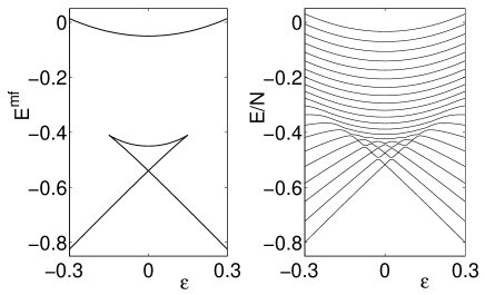
Figure 1: Total energy (5) in the mean-field theory (left) and eigenenergies the many-particle Hamiltonian (6),(right) for $v=0.2$, $g=-1$ and $N=20$ particles.

Going back to the roots of the problem, we consider the original many-particle problem of an interacting two-mode boson field instead of the mean-field theory. We consider the many-particle Hamiltonian of Bose-Hubbard type,

$$\hat{H}(t) = \epsilon(t)(\hat{n}_{1}-\hat{n}_{2})+v(\hat{a}_{1}^{\dagger}\hat{a}_{2}+\hat{a}_{2}^{\dagger}\hat{a}_{1})$$ (6)

$$\quad+\frac{\bar{g}}{2}(\hat{n}_{1}(\hat{n}_{1}-1)+\hat{n}_{2}(\hat{n}_{2}-1)),$$

where $\hat{a}_{j}$ and $\hat{a}_{j}^{\dagger}$ are the bosonic annihilation and creation operators in the $j$th well and $\hat{n}_{j}=\hat{a}_{j}^{\dagger}\hat{a}_{j}$ is the occupation number operator. The eigenvalues of the Hamiltonian (6) are shown in Fig. 1 on the right-hand side in dependence of $\epsilon$ for $g=-1$, $v=0.2$ and $N=20$ particles. One recognizes the similarity to the mean-field results shown on the left-hand side. A series of avoided crossings with very small level distances is observed where the mean-field energy levels form the swallow’s tail structure.

For $t\rightarrow-\infty$, one has $\epsilon=\alpha t\rightarrow-\infty$ and the first term dominates the Hamiltonian. The ground state is $|\psi_{0}\rangle=(N!)^{-1/2}(\hat{a}_{1}^{\dagger})^{N}|0\rangle$, where $N$ is the fixed number of particles. In the spirit of the Landau-Zener problem we take this as the initial state for $t\rightarrow-\infty$ and consider the question, how many particles remain in the first well for $t\rightarrow+\infty$, i.e. the effective Landau-Zener transition probability for the population, which is given by

$$P_{\rm LZ}^{\rm mp}=\frac{\langle\hat{n}_{1}(t\rightarrow+\infty)\rangle}{\langle\hat{n}_{1}(t\rightarrow-\infty)\rangle}\,.$$ (7)

The superscripts mp and mf are introduced to distinguish between the many-particle and the mean-field system. It will be shown that this many-particle Landau-Zener probability agrees well with the mean-field Landau-Zener probability (3). Furthermore this ”back-to-the-roots”-procedure reduces the problem to a linear multi-level Landau-Zener scenario, which can be solved approximately in an independent crossing approximation. In this way we derive a Landau-Zener formula for an interacting BEC, which agrees well with numerical results especially in the strongly interacting regime $|g|>g_{c}=2v$.

II The many-particle Landau-Zener problem and the ICA

We now consider the many-particle Landau-Zener scenario (6) in detail, where the number $N$ of particles is fixed. We expand the Hamiltonian $H$ in the number-state basis $|k\rangle=[k!(N-k)!]^{-1/2}(\hat{a}_{1}^{\dagger})^{k}(\hat{a}_{2}^{\dagger})^{N-k}|0\rangle$. Then the Hamiltonian is given by the matrix $\langle\ell|H|k\rangle=H_{\ell,k}$ for $\ell,k=0,\ldots,N$ with the elements

$$H_{\ell,k}=h_{\ell}(t)\,\delta_{\ell,k}+v_{\ell}\,(\delta_{\ell,k-1}+\delta_{\ell-1,k})$$ (8)

and

$$h_{\ell}(t)=\epsilon(t)(2\ell-N)+\frac{\bar{g}}{2}(2\ell^{2}-2\ell N+N^{2}-N)$$

and the couplings $v_{\ell}=v\sqrt{(\ell+1)(N-\ell)}$ on the sub- and superdiagonal. In the Landau-Zener scenario, all diabatic (i.e. uncoupled) levels $h_{\ell}(t)$ vary linearly in time as $\epsilon(t)=\alpha t$, however with a different offset and slope $\alpha(2\ell-N)$.

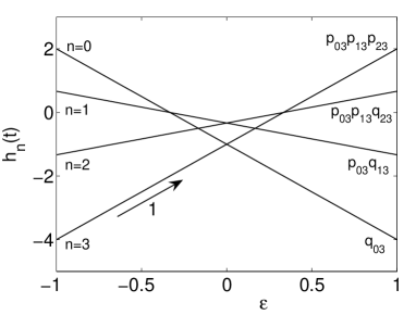
Figure 2: The S-matrix elements $|S_{\ell,N}|^{2}$ in the independent crossing approximation (ICA) for $N=3$ particles.

As stated above, we assume that initially all particles are in the first well, $|\psi(t\rightarrow-\infty)\rangle=|N\rangle$. Consequently one has $\langle\hat{n}_{1}(t\rightarrow-\infty)\rangle=N$ and in order to derive the Landau-Zener probability (7) we are left with the problem to calculate $\langle\hat{n}_{1}(t\rightarrow+\infty)\rangle$. Thus we are not interested in the details of the time evolution. We just need a few elements of the $S$-matrix, which is defined by

$$\langle k|\psi(t=+\infty)\rangle=\sum_{\ell}S_{k\ell}\langle\ell|\psi(t=-\infty)\rangle.$$ (9)

With this definition and $\langle\ell|\hat{n}_{1}|k\rangle=k\delta_{\ell,k}$, the Landau-Zener transition probability (7) is reduced to

$$P_{\rm LZ}^{\rm mp}=\frac{1}{N}\sum_{k=0}^{N}k|S_{k,N}|^{2}\,,$$ (10)

so that only the squared modulus of the $S$-matrix elements $|S_{k,N}|^{2}$ are of importance.

The S-matrix elements $|S_{N,k}|^{2}$ are now evaluated in a modified independent crossings approximation (ICA, see appendix for details). One assumes that the system undergoes a series of single, independent transitions between just two levels. The probabilities of a diabatic resp. adiabatic transition at a single anti-crossing are given $p_{k,N}=\exp(-\pi w_{k,\ell}^{2}/|b_{k,l}|)$ resp. $q_{k,\ell}=1-p_{k,\ell}$ according to the Landau-Zener formula (4). Here, $w_{k,l}$ denotes the level spacing at the anti-crossing and $b_{k,\ell}$ is the difference of the slopes of the two diabatic levels. The relevant S-matrix elements are given by

$$|S_{k,N}|^{2}=(1-p_{k,N})\prod_{\ell=0}^{k-1}p_{\ell,N}\,,$$ (11)

with the definition $q_{NN}=1\Leftrightarrow p_{NN}=0$. The calculation of the S-matrix elements by the ICA is illustrated in Fig. 2 for the case $N=3$.

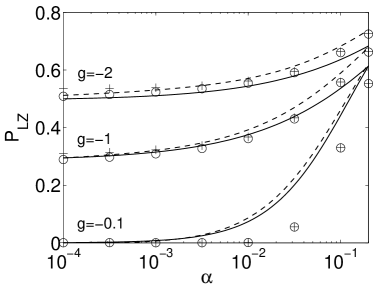
Figure 3: Landau-Zener tunneling probability in dependence of the parameter velocity $\alpha$ for $v=0.2$, $N=100$ particles and different values of the interaction constant $g$. Numerical data (mean-field $+$ and many-particle theory $\circ$) is compared with the ICA (12),(dashed line) and the resulting ICA-Landau-Zener formulae (25) resp. (26),(solid line).

The ICA-Landau-Zener transition probability is then given by

$$P_{\rm LZ}^{\rm ICA} = \frac{1}{N}\sum_{k=0}^{N}k(1-p_{k,N})\prod_{\ell=0}^{k-1}p_{\ell,N}$$ (12)

$$= \frac{1}{N}\sum_{k=0}^{N-1}\prod_{\ell=0}^{k}p_{\ell,N}\,.$$

Note that the $p_{\ell,N}$ depend on the distance between the levels $\ell$ and $N$ at the anti-crossing. Thus they have to be evaluated at different times $t_{\ell,N}$. However, the crossing time is easily calculated by evaluating $h_{N}(t_{\ell,N})=h_{\ell}(t_{\ell,N})$, where $h_{\ell}(t)$ are diabatic levels as defined above. This yields

$$t_{\ell,N}=-\frac{\bar{g}\ell}{2\alpha}\,.$$ (13)

At all crossing times $t_{\ell,N}$, the level spacings $w_{\ell,N}$ are calculated by diagonalizing the Hamiltonian matrix (8). As $H$ is tridiagonal, this can be done very efficiently. Furthermore, the difference of the slopes is simply given by $b_{\ell,N}=2\alpha(N-\ell)$.

To test this approach we compare the ICA-Landau-Zener formula (12) with the Landau-Zener probability (7) calculated by numerically integrating the many-particle Schrödinger equation as well as the mean-field transition probability (3). The results are shown in Fig. 3 in dependence of $\alpha$ for $v=0.2$, $N=100$ and three different values of $g$. One observes a good agreement between the Landau-Zener formula (12),(dashed line) and the numerical results for large $g$. For small values of $g$ the ICA (12) overestimates the transition probability. These issues will be further discussed in section V.

III Limiting cases

The linear limit $g\rightarrow 0$ is analytically solvable in both cases. The many-particle system (8) reduces to the so-called bow-tie model, whose S-matrix was calculated in Demk01 . The mean-field dynamics reduces to the ordinary two-state model of Landau, Zener, Majorana and Stückelberg Land32 ; Zene32 ; Majo32 ; Stue32 . Not only the transition probability but also the whole dynamics is known exactly in terms of Weber functions Zene32 .

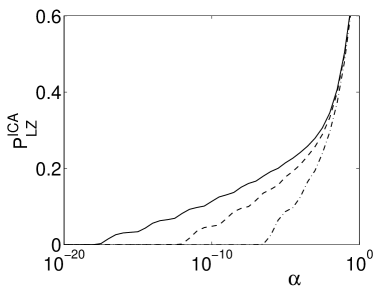
Figure 4: Landau-Zener transition probability $P_{\rm LZ}^{\rm ICA}(\alpha)$ in the adiabatic limit $\alpha\rightarrow 0$ for $v=0.2$, $g=-1$ and different numbers of particles: $N=10$ ($-\cdot-$), $N=20$ ($--$) and $N=30$ (—).

In the zero-coupling limit $v\rightarrow 0$ the Hamiltonians become diagonal and the evolution is fully diabatic. The Landau-Zener transition probability tends to one.

Most interesting is the adiabatic limit $\alpha\rightarrow 0$. As no subdiagonal element of the Hamiltonian matrix (8) vanishes, all eigenvalues must be distinct (see, e.g. Wilk65 ). They may become pathologically close, but they cannot be degenerate. This is in fact the case: The splitting of the lowest levels at the anti-crossings becomes really small for increasing $|\bar{g}|$. Thus all $w_{l,N}$ are non-zero and in the extreme adiabatic limit $\alpha\rightarrow 0$ the Landau-Zener probabilities $p_{\ell,N}$ must vanish. This seems to contradict the mean-field results (cf. Fig. 3), which predicts a non-zero Zener tunneling probability even in the adiabatic limit if $|g|>g_{c}$.

However, the parameter regime, where the ICA predicts a vanishing Zener tunneling probability in contrast to the mean-field results, decreases rapidly with an increasing number of particles $N$. Figure 4 shows the Landau-Zener probability $P_{\rm LZ}^{\rm ICA}(\alpha)$ for very small $\alpha$, calculated within the ICA for different $N$, with $g=\bar{g}N=-1$ fixed. The truly adiabatic region, where $P_{\rm LZ}^{\rm ICA}(\alpha)\approx 0$ is negligibly small already for these quite modest numbers of $N$.

The mean-field theory is valid for a BEC consisting of a macroscopic number of atoms. In order to compare to the mean-field results we thus have to consider the limit of a large number of particles, $N\rightarrow\infty$ with $g=\bar{g}N$ fixed. In this macroscopic limit, the contradiction vanishes. Furthermore, this limit will prove itself as extremely convenient for the evaluation of Eq. (12), since all sums can be replaced by integrals which can be solved explicitly (cf. section V).

IV The many-particle spectrum

The only missing step towards an explicit Landau-Zener formula is the evaluation of the squared levels spacings $w^{2}_{k,N}(t_{k,N})$. Thus one has to understand the spectrum of the Hamiltonian (6). We start with a discussion of the spectrum for $\epsilon=0$, which provides an insight into the qualitative features which will guide us in the following. To keep the calculations simple, we introduce the operators

$$J_{x} = \frac{1}{2}\left(a_{2}^{\dagger}a_{2}-a_{1}^{\dagger}a_{1}\right)$$

$$J_{y} = \frac{{\rm i}}{2}\left(a_{2}^{\dagger}a_{1}-a_{1}^{\dagger}a_{2}\right)$$

$$J_{z} = \frac{1}{2}\left(a_{1}^{\dagger}a_{2}+a_{2}^{\dagger}a_{1}\right),$$ (14)

which form an angular momentum algebra with quantum number $j=N/2$ Milb97 ; Vard01b ; Angl01 . The Hamiltonian (6) then can be rewritten as

$$H=2vJ_{z}+\frac{g}{N}J_{x}^{2}$$ (15)

up to a constant term.

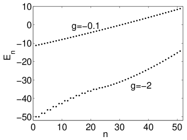
Figure 5: Spectrum of the many-particle Hamiltonian (6) for $\epsilon=0$, $v=0.2$, $N=50$ particles and $g=-0.1$ and $g=-2$, respectively.

In the subcritical case $|g|<2|v|$, the interaction terms can be treated as a small perturbation. The unperturbed eigenstates are the $J_{z}$-eigenstates $|j,m_{z}\rangle$ with $m_{z}=-j,-j+1,\ldots,j$. In second order this yields the levels

$$E_{m_{z}}=2vm_{z}\left[1-\frac{g}{2v}\frac{m_{z}}{2N}-\left(\frac{g}{2v}\right)^{2}\frac{m_{z}^{2}}{4N^{2}}+\mathcal{O}(g^{3})\right]$$ (16)

up to a constant. This spectrum is illustrated in Fig. 5 for $g=-0.1$, $v=0.2$ and $N=50$ particles. The eigenenergies are nearly equidistant, with a slight increase of the level spacing for higher energies.

For $|g|>2|v|$ and low energies, the interaction term $gJ_{x}^{2}/N^{2}$ dominates the Hamiltonian. The eigenstates with quantum numbers $|j,\pm m_{x}\rangle$ are doubly degenerate with eigenenergy $E_{m_{x}}=gm_{x}^{2}/N^{2}$. The perturbation $2vJ_{z}$ removes this degeneracy only in the $2|m_{x}|$-th order. Thus the low energy eigenstates (corresponding to the high $|m_{x}|$ states) appear in nearly degenerate pairs. However this approach fails if the energy scale of the perturbation $2vJ_{z}$ becomes comparable to the unperturbed eigenenergy. Estimating the energy scale of the perturbation as $E_{\rm max}/2=2vj/2$, perturbation theory fails for $|g|m_{x}^{2}/N^{2}\apprle vN/2$. Instead, Bogoliubov theory provides the appropriate description for the high energy part of the spectrum. We are dealing with an attractive interaction $g<0$, so that the highest state in the mean-field approximation is the state with equal population in the two modes. So the standard Bogoliubov approach is valid for the highest state instead of the ground state. One finds that the high energy part of the spectrum is given by $E_{n}=E_{N}-\omega(N-n)$ with the Bogoliubov frequency Pita03

$$\omega=[(2v)^{2}-2vg]^{1/2}.$$ (17)

To clarify this issue, the spectrum is plotted in Fig. 5 for $g=-2$, $v=0.2$ and $N=50$ particles. One clearly sees the nearly degenerate pairs of eigenvalues for low energies and the approximately equal spacing of the high-energy eigenvalues. The distance of the two highest levels is given by the Bogoliubov frequency (17).

Now we come back to the squared level splittings $w_{k,N}^{2}(t_{k,N})$, beginning with the supercritical regime $|g|>2v$. Figure 6 shows an example of the squared level splitting for $v=0.2$, $N=100$ particles and $g=-0.1$ resp. $g=-1$. Later, we consider the macroscopic limit $N\rightarrow\infty,\;\bar{g}\rightarrow 0$ with $g=\bar{g}N$ fixed. For this issue we plot the squared level splittings versus the rescaled index $x:=\ell/N\in[0,1]$. With increasing $N$, the curve plotted in Fig. 6 remains the same, only the actual points move closer together. Thus one obtains a continuous function $w^{2}(x)$ in the limit $N\rightarrow\infty$.

As argued above for $\epsilon=0$, the lower levels appear in approximately degenerate pairs. By the same arguments one concludes that this is also true for for the first level crossings. Thus, $w^{2}_{\ell,N}$ is effectively zero for $\ell<\ell_{c}$ resp. $x<x_{c}$. The critical index $x_{c}$ can be estimated as described above for $\epsilon=0$. It is found that this estimate gives the correct results up to a numerical factor $a$ of order 1. Thus we conclude that

$$x_{c}\approx 1-a\sqrt{2v/|g|}.$$ (18)

A very good agreement of this formula to the numerical results was found for $a=1.14$.

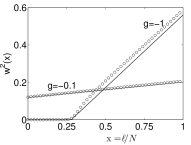
Figure 6: Squared level splitting $w^{2}(x)$ in dependence of the scaled index $x=\ell/N$ for $v=0.2$ and $g=-0.1$ resp. $g=-1$. Numerical results ($\circ$) are compared to the approximate formulae (19) resp. (20), (solid lines).

For $x>x_{c}$ the squared splittings increase approximately linear. In the high energy limit corresponding to $x\rightarrow 1$, the level splitting is given by the Bogoliubov frequency introduced above. In conclusion, the squared level spacing can be approximated by

$$w^{2}(x)\approx\omega^{2}\frac{x-x_{c}}{1-x_{c}}H(x-x_{c}),$$ (19)

where $H(x-x_{c})$ denotes Heaviside’s step function.

In the subcritical regime $|g|<2v$, one can use the results from perturbation theory described above (cf. Eq. (16)). At time $t_{\ell,N}=-\bar{g}\ell/2\alpha$ one must evaluate the level splitting $E_{\ell-j+1}-E_{\ell-j}$ (note that the levels are labeled by $m_{z}=-j,-j+1,\ldots,j$ with $j=N/2$). Again we consider the limit $N\rightarrow\infty$ with $g=\bar{g}N$ fixed. After a little algebra one finds that the relevant level splitting is in linear order given by

$$w(x) = \frac{16v^{2}+4g-3g^{2}/4}{8v}+\left(\frac{3g^{2}}{8v}-g\right)x$$ (20)

$$=: w_{0}+w_{1}x$$

in terms of the scaled index $x=\ell/N$.

The approximate results for the squared level splitting $w^{2}(x)$ for $|g|>g_{c}$, Eq. (19), and for $|g|<g_{c}$, Eq. (20), are compared with the numerical results for $N=100$ particles in Fig. 6. One observes a good agreement.

V Towards an explicit Landau-Zener formula

Using the formulae for the squared level splitting derived in the previous section, the ICA-Landau-Zener transition probability (12) can now be evaluated explicitly. In the spirit of the of the macroscopic limit $N\rightarrow\infty$, the sums are replaced by integrals according to

$$\frac{1}{N}\sum_{\ell=0}^{k}\rightarrow\int_{0}^{k/N}dx$$ (21)

The difference of the slopes $b_{\ell,N}=2\alpha(N-\ell)$, which enters the formula is also rewritten in terms of the rescaled index $x=\ell/N$:

$$b_{\ell,N}\rightarrow 2\alpha N(1-x)=:N\bar{b}(x).$$ (22)

Thus one finds

$$P_{LZ}\approx\int_{0}^{1}\exp\left[-\pi\int_{0}^{y}\frac{w^{2}(x)}{\bar{b}(x)}dx\right]dy.$$ (23)

In the supercritical regime $|g|>g_{c}$ we start by evaluating the integral over $x$ in Eq. (23). Substituting $w^{2}(x)$ and $\bar{b}(x)$ from Eq. (19) and (22) and carrying out the integral yields

$$\int_{0}^{y}\frac{w^{2}(x)}{\bar{b}(x)}dx=\frac{-\omega^{2}}{2\alpha}\left[\frac{y-x_{c}}{1-x_{c}}+\ln\left(\frac{1-y}{1-x_{c}}\right)\right]$$ (24)

for $y>x_{c}$ and zero otherwise. The Landau-Zener transition probability (23) is then given by

$$P_{\rm LZ} \approx x_{c}+\int_{x_{c}}^{1}\left(\frac{1-y}{1-x_{c}}\right)^{\frac{\pi\omega^{2}}{2\alpha}}\exp\left[\frac{\pi\omega^{2}}{2\alpha}\frac{y-x_{c}}{1-x_{c}}\right]dy$$ (25)

$$= x_{c}+\frac{(1-x_{c})\,{\rm e}^{u}}{u^{u+1}}\,\gamma(u+1,u)$$

with the abbreviation $u=\pi\omega^{2}/2\alpha$ and $x_{c}$ defined in Eq. (18). Here, $\gamma$ denotes the incomplete gamma-function Abra72 .

In the subcritical regime $|g|<g_{c}$, one finds by substituting Eq. (23) into (23), that the Landau-Zener transition probability is given by

$$P_{LZ}\approx\int_{0}^{1}\left(1-y\right)^{(\pi w_{0}(w_{0}+2w_{1}))}\exp\left[2\pi w_{0}w_{1}y\right]dy$$

$$\;=\frac{{\rm e}^{c_{1}}}{c_{1}^{c_{0}+1}}\,\gamma\left(c_{0}+1,c_{1}\right)$$ (26)

with the abbreviations $c_{0}=\pi(w_{0}^{2}+2w_{0}w_{1})/2\alpha$ and $c_{1}=\pi w_{0}w_{1}/\alpha$. To keep the calculations feasible, we kept only terms linear in $x$ resp. $y$ in the exponent consistent with Eq. (25).

To test the validity of our approach we compare the ICA-Landau-Zener formulae (25) and (26) to numerical results obtained by integrating the Schrödinger equation for mean-field Hamiltonian (2) as well as the many-particle Hamiltonian (6). The Landau-Zener tunneling probability in dependence of the interaction constant $g$ is plotted in Fig. 7 for $\alpha=0.01$ in dependence of the velocity parameter $\alpha$ for different values of $g$ in Fig. 3.

One observes a good agreement of the ICA-Landau-Zener formula with the numerical results in the critical regime $|g|>g_{c}$. Especially the increase of the tunneling probability with increasing $|g|$ for small $\alpha$ is well described by our model. This problem could not be solved with previous approaches Zoba00 ; Liu02 . The approximation gets worse for larger values of $\alpha$ because the assumption that the Zener transitions are well separated becomes doubtful for such a large parameter velocity. The ICA thus underestimates the tunneling probability.

In the subcritical case $|g|<g_{c}$, the proposed ICA-Landau-Zener formula does not work as well. In fact the tunneling probability is overestimated for small $\alpha$ because the ICA itself is not a very good approximation in this case. The adiabatic levels do not show well separated avoided crossings, instead the levels splittings are nearly constant over a long interval of the parameter $\epsilon$. For larger values of $\alpha$ one faces the same problems as in the supercritical case and the tunneling probability is underestimated. Another ansatz, using e.g. perturbation theory with respect to the solution of the noninteracting problem Angl03 should be better suited to this problem. Note however, that the deviations are mainly due to the ICA itself and to the approximation of $w^{2}(x)$ made in this section.

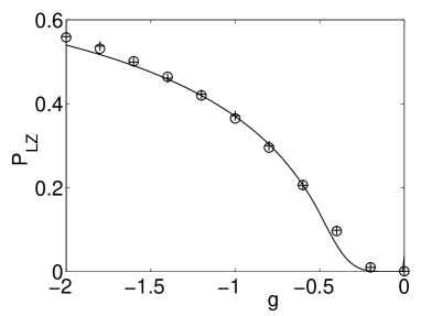
Figure 7: Landau-Zener tunneling probability in dependence of the interaction constant $g$ for a parameter velocity $\alpha=0.01$. Numerical data (mean-field $+$ and many-particle theory $\circ$) is compared to the ICA-Landau-Zener formula (25),(solid line) for $v=0.2$.

VI Conclusion and Outlook

In conclusion, we have derived a Landau-Zener formula for an interacting Bose-Einstein condensate from first principles. To this end we considered the original two-mode many-particle Landau-Zener scenario. It was shown that the resulting Landau-Zener formula agrees well with the numerical results calculated for the many-particle problem as well as within the mean-field approximation.

In the future, it would be of interest to relate our calculations to the respective problem in the Heisenberg pictures. Here, complex eigenfrequencies may occur for the dynamics of the creation/annihilation operators, leading to spontaneous production of quasi-particles and hence a dynamical instability. For the non-interacting case, this problem has been solved analytically Angl03 .

Another issue is the discussion of nonlinear Landau-Zener problems for more than two levels. First results for three level system were reported only recently 05level3 .

Appendix: The independent crossings approximation

Let us first briefly recall the dynamics of a two-level Landau-Zener system described by the Hamiltonian

$$H_{0}(t)=\left(\begin{matrix}\beta_{1}t+b_{1}&v\\ v&\beta_{2}t+b_{2}\end{matrix}\right).$$ (27)

The diabatic and adiabatic energy curves are plotted in Fig. 8. The S-Matrix in the sense of Eq. 9 is given by

$$S=\left(\begin{matrix}p&q\\ q&p\end{matrix}\right)$$ (28)

with $p=\exp{\left(-\pi v^{2}/|\beta_{1}-\beta_{2}|\right)}$ and $q=\sqrt{1-p^{2}}$. The probability of a diabatic passage is therefore given by the Landau-Zener-formula $P_{\rm LZ}=p^{2}=\exp{\left(-\frac{2\pi v^{2}}{|\beta_{1}-\beta_{2}|}\right)}$, and the adiabatic transition probability by $1-P_{\rm LZ}=q^{2}$. They depend only on the relative slope of the diabatic levels $|\beta_{1}-\beta_{2}|$ and the coupling $v$, which is equivalent to half of the gap between the adiabatic energy-levels at the avoided crossing.

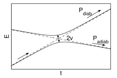
Figure 8: Diabatic (dash-dotted line) and adiabatic (solid line) energy levels of the two-level Landau-Zener model (27).

The simplicity of the solution of the two-level system and the observation that the transitions between two adiabatic levels in a multilevel Landau-Zener system takes place only in a very narrow region around the crossing of the two corresponding diabatic levels leads to a simple approximation. If all crossings are well separated they can be considered as independent of each other and each of them is described by the two-level-Landau-Zener model where the couplings between the relevant diabatic levels are given by the nondiagonal terms of the Hamiltonian. This approach is called the "independent crossing approximation" (ICA) in the literature. It is of great importance for the study of multilevel Landau-Zener dynamics because of a surprising feature: The ICA turns out to give the exact results for all known exactly solvable multi-level Landau-Zener scenarios Demk68 ; Demk01 . Furthermore it has been shown that the ICA always gives the correct results for the diagonal $S$-matrix elements with minimal and maximal slope Sini04 ; Shyt04 .

Of course there are also examples where the ICA fails, as for example for the simple three level Hamiltonian

$$H(t)=\left(\begin{matrix}\alpha t+a&v&w\\ v&0&0\\ w&0&-\alpha t+a\end{matrix}\right).$$ (29)

The adiabatic and diabatic levels are plotted in figure 9. The diabatic transition probability for the third level $S_{33}$ is exactly given by the ICA. But if we look at the S-Matrix element $S_{32}$ we find that the ICA predicts it to be zero, because the coupling matrix element vanishes, $\langle 2|H|3\rangle=0$, independent of $\alpha$ and $a$, which isn’t true. The second and the third diabatic levels do not couple directly, but for not too large values of $a$ the indirect coupling via the second diabatic level can’t be neglected. This coupling manifests itself as an avoided crossing between the two adiabatic levels, which turns into a real crossing only in the limits $a\to\infty$ and $a\to 0$. For finite values of $a$ the transition probability between the third and the second diabatic levels is small but nonzero.

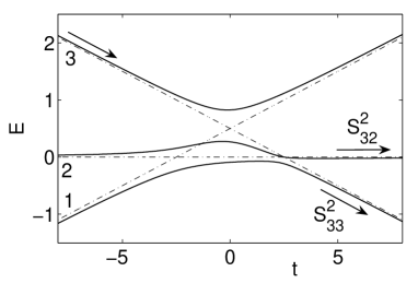
Figure 9: Diabatic (dash-dotted line) and adiabatic (solid line) energy levels of the three-level Landau-Zener model (29) for $\alpha=0.2$, $a=0.5$, $v=0.2$ and $w=0.3$.

To get a better approximation one should recall the two level system, where the coupling between two diabatic levels is equivalent to half of the level-splitting of the corresponding adiabatic levels. Therefore one can use a modified ICA where the couplings are not given by the nondiagonal elements of the Hamiltonian but half of the level splitting between the relevant adiabatic levels. This approximation doesn’t inherit the benefit of providing the exact results in the special cases where the original ICA did, but provides a good approximation even in the cases where the ICA fails. Therefore it is better suited for our purposes. The performance of the approximation is limited by the fact that the single avoided crossings must be well separated so that the transition regimes do not overlap. In the present case this is improved with increasing nonlinearity. Note that to simplify matters this modified ICA is denoted as ICA throughout the paper.

- (1) Biao Wu and Qian Niu, Phys. Rev. A 61, 023402 (2000).
- (2) Biao Wu and Qian Niu, New J. Phys. 5, 104 (2003).
- (3) J. Liu, B. Wu, and Q. Niu, Phys. Rev. Lett. 90, 170404 (2003).
- (4) L. D. Landau, Phys. Z. Sowjet. 1, 88 (1932).
- (5) C. Zener, Proc. Roy. Soc. Lond. A 137, 696 (1932).
- (6) E. Majorana, Nuovo Cim. 9, 43 (1932).
- (7) E. C. G. Stückelberg, Helvetica Physica Acta 5, 369 (1932).
- (8) B. Esser and H. Schanz, Z. Phys. B 96, 553 (1995).
- (9) O. Zobay and B. M. Garraway, Phys. Rev. A 61, 033603 (2000).
- (10) J. Liu, D. Choi, B . Wu and Q. Niu, Phys. Rev. A 66, 023404 (2002).
- (11) Yu. N. Demkov and V. N. Ostrovsky, J. Phys. B 34, 2419 (2001).
- (12) J. H. Wilkinson, The Algebraic Eigenvalue Problem (Oxford University Press, Oxford, 1965).
- (13) G. J. Milburn, J. Corney, E. M. Wright, and D. F. Walls, Phys. Rev. A 55, 4318 (1997).
- (14) A. Vardi and J. R. Anglin, Phys. Rev. Lett. 86, 568 (2001).
- (15) J. R. Anglin and A.Vardi, Phys. Rev. A 64, 013605 (2001).
- (16) L. Pitaevskii and S. Stringari, Bose-Einstein Condensation (Oxford University Press, Oxford, 2003).
- (17) M. Abramowitz and I. A. Stegun, Handbook of Mathematical Functions (Dover Publications, Inc., New York, 1972).
- (18) J. R. Anglin, Phys. Rev. A 67, 051601(R) (2003).
- (19) E. M. Graefe, H. J. Korsch, and D. Witthaut, Phys. Rev. A, in press (preprint: quant–ph/0507185) (2005).
- (20) Y. N. Demkov and V. I. Osherov, Sov. Phys. JETP 26, 916 (1968).
- (21) N. A. Sinitsyn, J. Phys. A 37, 10691 (2004).
- (22) A. V. Shytov, Phys. Rev. A 70, 052708 (2004).