Quantum Mechanics of Klein-Gordon Fields II:
Relativistic Coherent States

Abstract

We use the formulation of the quantum mechanics of first quantized Klein-Gordon fields given in the first of this series of papers to study relativistic coherent states. In particular, we offer an explicit construction of coherent states for both charged and neutral (real) free Klein-Gordon fields as well as for charged fields interacting with a constant magnetic field. Our construction is free from the problems associated with charge-superselection rule that complicated the previous studies. We compute various physical quantities associated with our coherent states and present a detailed investigation of their classical (nonquantum) and nonrelativistic limits.

1 Introduction

The study of the relationship between classical and quantum mechanics (QM) has been among the most important issues of modern theoretical physics. A related subject of great significance that has been the focus of attention since the very early days of QM is that of coherent states. Introduced by Schrödinger [1] as early as in 1926 and systematically formulated and developed in the capable hands of Glauber [2], Sudarshan [3], and Klauder [4] in the 1960s, coherent states have found widespread applications in various branches of physics, extending from particle physics to quantum optics [5, 6, 7, 8] and more recently quantum computation [9].

The conceptual and practical significance of coherent states have naturally motivated the introduction and study of their generalizations. Probably the most notable of these has been the development of coherent states associated with general Lie algebras [4, 10, 11, 6, 7]. Another basic problem has been to explore the relativistic coherent states. The purpose of the present paper is to employ the formulation of the QM of Klein-Gordon (KG) fields developed in [12], to provide an explicit construction of relativistic coherent states for first-quantized KG fields [13, 14, 15, 16].

Our basic point of departure, besides the general formalism developed in [12], is Glauber’s description of nonrelativistic coherent states [2], according to which one may use any one of the following equivalent definitions: 1) The coherent state vectors $|\zeta\rangle$ are eigenvectors of the (harmonic-oscillator) annihilation operator $a$, $a|\zeta\rangle=\zeta|\zeta\rangle$; 2) $|\zeta\rangle$ can be obtained by applying the Glauber’s displacement operator $D(\zeta):=\exp(\zeta a^{\dagger}-\zeta^{*}a)$ on the vacuum state vector $|0\rangle$, $|\zeta\rangle=D(\zeta)|0\rangle$; 3) $|\zeta\rangle$ determines a quantum state with a minimum-uncertainty relationship, $\Delta p~{}\Delta q=\hbar/2$, where $q,p$ are the canonically conjugate coordinate and momentum operators, $\Delta O:=\sqrt{\langle\zeta|O^{2}|\zeta\rangle-\langle\zeta|O|\zeta\rangle^{2}}$ for an observable $O$, and $|\zeta\rangle$ is assumed to be normalized.

A key issue in the construction of coherent states is the identification of an appropriate canonically conjugate pair of coordinate and momentum operators. For a nonrelativistic particle having $\mathbb{R}^{n}$ as its configuration space, these are usually the position and momentum operators in a Cartesian coordinate system. But in general one may make other choices. A typical example is the choice made in Re. [13] where the authors use the symmetries of the problem to select a pair of annihilation operators that do not correspond to the usual choice of coordinate and momentum operators. The problem of determining coordinate and momentum operators is at the heart of much of the difficulties encountered in constructing a physically viable candidate for relativistic coherent states. This is mainly because the identification of an appropriate relativistic position operator has been a nontrivial task [23, 24, 25, 26, 12].

The first thorough investigation of relativistic coherent states for first quantized KG fields is due to Bagrov, Buchbinder, and Gitman [14]. These authors express the KG equation in a certain null plane coordinate system as an equation which is first order in one of the coordinates and employ the idea of linear dynamical invariants of Malkin and Man’ko [13] to obtain a set of relativistic coherent states. These coherent states have certain appealing properties, but the corresponding coordinate operator does not coincide with any of the known relativistic position operators [23, 24].

In a more recent paper [15], Lev, Semenov, Uslenko, and Klauder construct a set of coherent states for KG fields interacting with a static magnetic field. Their analysis uses the position operator $q$ of [25, 27] that does not respect the charge superselection rule [28], i.e., its action mixes the negative- and positive-energy KG fields. To remedy this problem, Lev et al choose to construct the relativistic coherent states, for free KG fields, using the “even part” (the part that respects the charge superselection rule) of this position operator. This corresponds to the celebrated Newton-Wigner position operator [23]. The identification of $q$ with an observable causes certain peculiarity such as the possibility of a negative value for $\langle\zeta|q^{2}|\zeta\rangle$ and a subsequent violation of the minimum uncertainty relation.

The approach of [15] for treating coherent states for a KG field interacting with a constant magnetic field is based on the idea of nonlinear coherent states [29]. It involves the introduction of a deformed annihilation operator whose even part is used to construct a set of relativistic coherent states. This leads to some complications as the even part of the deformed annihilation and creation operators do not satisfy the usual commutation relations. Furthermore, this construction which relies on decoupling the translational and rotational degrees of freedom encounters the difficulty that the even part of the annihilation operators associated with these two degrees of freedom do not commute. This in turn necessitates the consideration of separate sets of coherent states corresponding to translational and rotational motions. These also display peculiar behaviors [15].

Refs. [26, 12] report on the construction of a set of relativistic position and momentum operators that respect the charge superselection rule. The eigenstates of the corresponding annihilation operator have a definite charge. Hence, they represent a set of coherent states that are free from the difficulties encountered in the above-mentioned studies. The purpose of the present paper is to perform a comprehensive investigation of the properties of these coherent states.

As we show in [12], we can apply our formulation for scalar fields interacting with an arbitrary stationary magnetic field by enforcing the minimal-coupling prescription, $\vec{\nabla}\rightarrow\vec{\nabla}-ie\vec{A}(\vec{x})$, in our treatment of free fields. In the presence of a nonstationary magnetic or a nonzero electric field, we are obliged to employ the nonstationary QM outlined in [30] and deal with the fact that the time-evolution is necessarily non-unitary. Therefore, in this paper we only consider, besides the free scalar fields, the charged scalar fields interacting with a constant homogeneous magnetic field.

The organization of the article is as follows. In Section 2 we outline a general construction for coherent states of a charged relativistic particle. In Section 3, we focus our attention on the coherent states of a free relativistic particle and examine their physical properties and classical and nonrelativistic limits. In Section 4, we study the coherent states of a neutral scalar particle. In Section 5, we consider the consequences of coupling a complex scalar field to a constant homogeneous magnetic field. Finally, in Section 6 we present our concluding remarks.

Throughout this paper we will occasionally refer to Ref. [12] as paper I and use the label (I-n) to denote Eq. (n) of paper I. Furthermore, we recall from paper I that the free KG equation may be expressed as

$$\ddot{\psi}(x^{0})+D\psi(x^{0})=0,$$ (1)

where $\psi(x^{0}):\mathbb{R}^{3}\to\mathbb{C}$ is defined by $\psi(x^{0})(\vec{x}):=\psi(x^{0},\vec{x})$ for all $x=(x^{0},\vec{x})\in\mathbb{R}^{4}$, an overdot stands for an $x^{0}$-derivative, $D:L^{2}(\mathbb{R}^{3})\to L^{2}(\mathbb{R}^{3})$ is the operator defined by $(D\phi)(\vec{x}):=(-\nabla^{2}+\mbox{\scriptsize${\cal M}$}^{2})\phi(\vec{x})$ for all $\phi\in L^{2}(\mathbb{R}^{3})$, and $\mbox{\scriptsize${\cal M}$}:=mc/\hbar$. As we mentioned earlier we may account for the interaction with a stationary magnetic field by letting $\vec{\nabla}\to\vec{\nabla}-ie\vec{A}(\vec{x})$ in the preceding formula for $D$, where $\vec{A}$ is the vector potential.

2 General Constructions for a Charged Scalar Field

Following paper I, Let ${\cal H}_{a}$ be the Hilbert space obtained by endowing the vector space ${\cal V}$ of solutions $\psi$ of the free KG equation (1), with the inner product

$$(\psi_{1},\psi_{2})_{a} = \frac{\kappa}{2\mbox{\scriptsize${\cal M}$}}\,\left\{\langle\psi_{1}(x^{0})|D^{1/2}\psi_{2}(x^{0})\rangle+\langle\dot{\psi}_{1}(x^{0})|D^{-1/2}\dot{\psi}_{2}(x^{0})\rangle+\right.$$ (2)

$$\hskip 42.67912pt\left.ia\left[\langle\psi_{1}(x^{0})|\dot{\psi}_{2}(x^{0})\rangle-\langle\dot{\psi}_{1}(x^{0})|\psi_{2}(x^{0})\rangle\right]\right\},$$

where $a\in(-1,1)$, $\kappa\in\mathbb{R}^{+}$, and $\psi_{1},\psi_{2}\in{\cal V}$ are arbitrary. As shown in [26] (See Eq. (I-42)), the Hilbert space ${\cal H}_{a}$ may be mapped onto the Hilbert space ${\cal H}^{\prime}:=L^{2}(\mathbb{R}^{3})\oplus L^{2}(\mathbb{R}^{3})$ of the two-component Foldy representation by a unitary transformation $U_{a}:{\cal H}_{a}\to{\cal H}^{\prime}$ of the form

$$U_{a}\psi \!\!\!\!:=\!\!\!\! \frac{1}{2}\sqrt{\frac{\kappa}{\mbox{\scriptsize${\cal M}$}}}\left(\begin{array}[]{c}\sqrt{1+a}~{}[D^{1/4}\psi(x^{0}_{0})+iD^{-1/4}\dot{\psi}(x^{0}_{0})]\\ \sqrt{1-a}~{}[D^{1/4}\psi(x^{0}_{0})-iD^{-1/4}\dot{\psi}(x^{0}_{0})]\end{array}\right)$$ (5)

$$\!\!\!\!=\!\!\!\! \frac{1}{2}\sqrt{\frac{\kappa}{\mbox{\scriptsize${\cal M}$}}}\,D^{1/4}\left(\begin{array}[]{c}\sqrt{1+a}~{}[\psi(x^{0}_{0})+\psi_{c}(x^{0}_{0})]\\ \sqrt{1-a}~{}[\psi(x^{0}_{0})-\psi_{c}(x^{0}_{0})]\end{array}\right),$$ (8)

where $x^{0}_{0}\in\mathbb{R}$ is a fixed initial value for $x^{0}=ct$ and $\psi_{c}(x^{0}):=iD^{-1/2}\dot{\psi}(x^{0})$. The inverse of $U_{a}$ is given by

$$\left[U_{a}^{-1}\xi\right](x^{0})=\sqrt{\frac{\mbox{\scriptsize${\cal M}$}}{\kappa}}\;D^{-1/4}\left[e^{-i(x^{0}-x^{0}_{0})D^{1/2}}\frac{\xi^{1}}{\sqrt{1+a}}+e^{i(x^{0}-x^{0}_{0})D^{1/2}}\frac{\xi^{2}}{\sqrt{1-a}}\right],$$ (9)

where $\xi=\mbox{\tiny$\left(\begin{array}[]{c}\xi^{1}\\ \xi^{2}\end{array}\right)$}\in{\cal H}^{\prime}$ and $x^{0}\in\mathbb{R}$ are arbitrary.

Denoting the $2\times 2$ identity matrix by $\sigma_{0}$, we can respectively express the position and momentum operators acting in ${\cal H}^{\prime}$ as

$$\vec{X}^{\prime}:=\vec{\rm x}\otimes\sigma_{0},~{}~{}~{}~{}~{}~{}~{}~{}~{}~{}\vec{P}^{\prime}:=\vec{\rm p}\otimes\sigma_{0},$$ (10)

where $\vec{\rm x}$ and $\vec{\rm p}$ are the ordinary position and momentum operator acting in $L^{2}(\mathbb{R}^{3})$. Next, we define the position ($\vec{X}_{a}$) and momentum ($\vec{P}_{a}$) operators and the associated annihilation operator ($\vec{A}_{a}$) acting in the Hilbert space ${\cal H}_{a}$ of the one-component KG fields by

$$\vec{X}_{a} := U_{a}^{-1}\vec{X}^{\prime}\,U_{a},~{}~{}~{}~{}~{}~{}~{}\vec{P}_{a}:=U_{a}^{-1}\vec{P}^{\prime}\,U_{a},$$ (11)

$$\vec{A}_{a} := \sqrt{\frac{k}{2\hbar}}\,\left(\vec{X}_{a}+ik^{-1}\vec{P}_{a}\right),$$ (12)

where $k=\texttt{{m}}\,\omega\in\mathbb{R}$ is the characteristic oscillator constant having the dimension of mass per time, [26]. We then identify the coherent states with the eigenstates of $\vec{A}_{a}$.

The charge-grading operator ${\cal C}^{\prime}$ and the charge operator ${\cal Q}^{\prime}$ acting in $\cal H^{\prime}$ are given by

$${\cal C}^{\prime}=\sigma_{3}=\left(\begin{array}[]{cc}1&0\\ 0&-1\end{array}\right),~{}~{}~{}~{}~{}~{}~{}~{}~{}~{}~{}~{}{\cal Q}^{\prime}:=e\sigma_{3},$$ (13)

where $e$ is the unit charge [26]. In view of (9) and ${\cal C}=U_{a}^{-1}{\cal C}^{\prime}U_{a}$, it is straightforward to calculate the charge-grading and charge operator acting in ${\cal H}_{a}$. The result is [26, 12]

$${\cal C}=iD^{-1/2}\frac{\partial}{\partial x^{0}},~{}~{}~{}~{}~{}~{}~{}~{}~{}~{}~{}~{}{\cal Q}:=e\,{\cal C}=ieD^{-1/2}\frac{\partial}{\partial x^{0}}.$$ (14)

As seen from these relations, ${\cal C}$ and ${\cal Q}$ do not depend on the parameter $a$. Furthermore, because ${\cal C}^{\prime},{\cal Q}^{\prime}:{\cal H}^{\prime}\to{\cal H}^{\prime}$ are Hermitian and $U_{a}:{\cal H}_{a}\to{\cal H}^{\prime}$ is unitary, ${\cal C},{\cal Q}:{\cal H}_{a}\to{\cal H}_{a}$ are Hermitian as well, i.e., they are physical observables.

Because both $\vec{X}_{a}$ and $\vec{P}_{a}$ commute with the charge-grading operator ${\cal C}$, so does the annihilation operator $\vec{A}_{a}$. This means that they respect the charge superselection rule [26, 12] and that the corresponding coherent states may be taken to have a definite charge. We will identify the latter with the common eigenstates of $\vec{A}_{a}$ and $\cal C$. The associated state vectors $\psi_{a}^{(\epsilon,\vec{\zeta}_{\epsilon})}$ satisfy

$$\vec{A}_{a}\>\psi_{a}^{(\epsilon,\vec{\zeta}_{\epsilon})}=\vec{\zeta}_{\epsilon}\>\psi_{a}^{(\epsilon,\vec{\zeta}_{\epsilon})},~{}~{}~{}~{}~{}~{}~{}~{}~{}~{}~{}~{}{\cal C}\>\psi_{a}^{(\epsilon,\vec{\zeta}_{\epsilon})}=\epsilon\>\psi_{a}^{(\epsilon,\vec{\zeta}_{\epsilon})},$$ (15)

where $\vec{\zeta}_{\epsilon}\in\mathbb{C}^{3}$ and $\epsilon=\pm$. By construction, the coherent state vectors $\psi_{a}^{(\epsilon,\vec{\zeta}_{\epsilon})}$ are free from the peculiarities associated with the nontrivial charge structure of the conventional coherent states [17, 18, 19, 13, 14, 15]. They are also solutions of the KG equation (1). We will refer to them as coherent Klein-Gordon fields.

Because the position operator $\vec{X}_{a}$ has a complicated form [26, 12], Eqs. (15) do not offer a practical method of computing $\psi_{a}^{(\epsilon,\vec{\zeta}_{\epsilon})}$. A more convenient method is to construct the corresponding coherent state vectors in the Foldy Representation, namely

$$|\vec{\zeta}_{\epsilon},\epsilon\rangle:=U_{a}\psi_{a}^{(\epsilon,\vec{\zeta}_{\epsilon})}.$$ (16)

2.1 Coherent States in Foldy Representation

In the Foldy representation, where the Hilbert space is ${\cal H}^{\prime}=L^{2}(\mathbb{R}^{3})\oplus L^{2}(\mathbb{R}^{3})$, the annihilation operator has the form

$$\vec{A}^{\prime}:=U_{a}\,\vec{A}_{a}\,U_{a}^{-1}=\sqrt{\frac{k}{2\hbar}}\,\left(\vec{X}^{\prime}+ik^{-1}\vec{P}^{\prime}\right).$$ (17)

In view of (11) – (13), (16) and (17),

$$\vec{A}^{\prime}|\vec{\zeta}_{\epsilon},\epsilon\rangle=\vec{\zeta}_{\epsilon}|\vec{\zeta}_{\epsilon},\epsilon\rangle,~{}~{}~{}~{}~{}~{}~{}~{}~{}{\cal C}^{\prime}|\vec{\zeta}_{\epsilon},\epsilon\rangle=\epsilon|\vec{\zeta}_{\epsilon},\epsilon\rangle,~{}~{}~{}~{}~{}~{}~{}~{}~{}|\vec{\zeta}_{\epsilon},\epsilon\rangle=|\vec{\zeta}_{\epsilon}\rangle\otimes e_{\epsilon},$$ (18)

where $e_{+}:=\mbox{\tiny$\left(\begin{array}[]{c}1\\ 0\end{array}\right)$}$, $e_{-}:=\mbox{\tiny$\left(\begin{array}[]{c}0\\ 1\end{array}\right)$}$, and $|\vec{\zeta}_{\epsilon}\rangle$ are the ordinary coherent state vectors satisfying

$$\vec{a}|\vec{\zeta}_{\epsilon}\rangle=\vec{\zeta}_{\epsilon}|\vec{\zeta}_{\epsilon}\rangle,~{}~{}~{}~{}{\rm with}~{}~{}~{}~{}\vec{a}:=\sqrt{\frac{k}{2\hbar}}\,\left(\vec{\rm x}+ik^{-1}\vec{\rm p}\right).$$ (19)

Next, we use the (complete and orthonormal) position basis vectors $\xi_{\epsilon,\vec{x}}:=|\vec{x}\rangle\otimes e_{\epsilon}$ of ${\cal H}^{\prime}$ to introduce the coherent wave function $f^{(\vec{\zeta}_{\epsilon},\epsilon)}$ as

$$f^{(\vec{\zeta}_{\epsilon},\epsilon)}(\epsilon^{\prime},\vec{x}):=\langle\xi_{\epsilon^{\prime},\vec{x}}|\vec{\zeta}_{\epsilon},\epsilon\rangle=\langle\vec{x}|\vec{\zeta}_{\epsilon}\rangle\,\delta_{\epsilon^{\prime},\epsilon}=f_{{}_{\rm coh}}(\epsilon,\vec{x})\,\delta_{\epsilon^{\prime},\epsilon},$$ (20)

where $\epsilon,\epsilon^{\prime}=\pm$ and

$$f_{{}_{\rm coh}}(\epsilon,\vec{x}):=\langle\vec{x}|\vec{\zeta}_{\epsilon}\rangle=f^{(\vec{\zeta}_{\epsilon},\epsilon)}(\epsilon,\vec{x}).$$ (21)

As seen from this relation $f_{{}_{\rm coh}}(\epsilon,\vec{x})$ is the usual coherent state wave function of the nonrelativistic QM which according to (19) satisfies

$$\sqrt{\frac{k}{2\hbar}}\,\left(\vec{x}+k^{-1}\vec{\nabla}\right)f_{{}_{\rm coh}}(\epsilon,\vec{x})=\vec{\zeta}_{\epsilon}f_{{}_{\rm coh}}(\epsilon,\vec{x}).$$ (22)

In view of (20) and the completeness of the position kets $|\vec{x}\rangle$ (alternatively $\xi_{\epsilon,\vec{x}}$),

$$|\vec{\zeta}_{\epsilon},\epsilon\rangle=\int_{\mathbb{R}^{3}}d^{3}x\,|\vec{x}\rangle\langle\vec{x}|\vec{\zeta}_{\epsilon}\rangle\otimes e_{\epsilon}=\int_{\mathbb{R}^{3}}d^{3}x\,f_{{}_{\rm coh}}(\epsilon,\vec{x})\,\xi_{\epsilon,\vec{x}}.$$ (23)

Similarly, we can employ the momentum basis vectors $\xi_{\epsilon,\vec{p}}$ of ${\cal H}^{\prime}$, that fulfil

$$\xi_{\epsilon,\vec{p}}:=|\vec{p}\rangle\otimes e_{\epsilon},~{}~{}~{}~{}~{}~{}~{}\langle\xi_{\epsilon,\vec{p}},\xi_{\epsilon^{\prime},\vec{p}^{\prime}}\rangle=\delta_{\epsilon,\epsilon^{\prime}}\delta^{3}(\vec{p}-\vec{p}^{\prime}),~{}~{}~{}~{}~{}~{}~{}\sum_{\epsilon=\pm}\int_{\mathbb{R}^{3}}d^{3}p\>|\xi_{\epsilon,\vec{p}}\rangle\langle\xi_{\epsilon,\vec{p}}|=\sigma_{0},$$ (24)

to obtain the momentum representation of coherent states, namely $|\vec{\zeta}_{\epsilon},\epsilon\rangle=\int_{\mathbb{R}^{3}}d^{3}p\,f_{{}_{\rm coh}}(\epsilon,\vec{p})\,\xi_{\epsilon,\vec{p}}$, where

$$f_{{}_{\rm coh}}(\epsilon,\vec{p}):=\langle\vec{p}|\vec{\zeta}_{\epsilon}\rangle=\langle\xi_{\epsilon,\vec{p}}|\vec{\zeta}_{\epsilon},\epsilon\rangle=\frac{1}{(2\pi\hbar)^{3/2}}\int d^{3}x\>e^{-i\frac{\vec{p}}{\hbar}\cdot\vec{x}}\>f_{{}_{\rm coh}}(\epsilon,\vec{x}).$$ (25)

As it is well-known, $|\vec{\zeta}_{\epsilon}\rangle$ are normalizable, non-orthogonal, and overcomplete [2, 7]. Moreover they yield a resolution of the identity which is not unique [2]. A common choice for the latter is

$$\int|\vec{\zeta}_{\epsilon}\rangle\frac{d^{2}\zeta_{\epsilon}}{\pi}\langle\vec{\zeta}_{\epsilon}|=1,$$ (26)

where $d^{2}\zeta_{\epsilon}=d\Re(\zeta_{\epsilon})\;d\Im(\zeta_{\epsilon})$.

Two-component coherent state vectors $|\vec{\zeta}_{\epsilon},\epsilon\rangle=|\vec{\zeta}_{\epsilon}\rangle\otimes e_{\epsilon}$ share the properties of $|\vec{\zeta}_{\epsilon}\rangle$; with an appropriate normalization constant they satisfy

$$\langle\vec{\zeta}_{\epsilon},\epsilon|\vec{\zeta}^{\prime}_{\epsilon^{\prime}},\epsilon^{\prime}\rangle=\delta_{\epsilon\epsilon^{\prime}}\,\exp\left[\vec{\zeta}_{\epsilon}^{*}\cdot\vec{\zeta}^{\prime}_{\epsilon}-\frac{1}{2}(|\vec{\zeta}_{\epsilon}|^{2}+|\vec{\zeta}^{\prime}_{\epsilon}|^{2})\right]\,,~{}~{}~{}~{}~{}~{}\sum_{\epsilon=\pm}\int|\vec{\zeta}_{\epsilon},\epsilon\rangle\,\frac{d^{2}\zeta_{\epsilon}}{\pi}\,\langle\vec{\zeta}_{\epsilon},\epsilon|=\sigma_{0}\,.$$ (27)

Using these properties, we can express any two-component vector $\Psi\in{\cal H}^{\prime}$ in the coherent state basis $\{|\vec{\zeta}_{\epsilon},\epsilon\rangle\}$ as

$$\Psi=\sum_{\epsilon=\pm}\int|\vec{\zeta}_{\epsilon},\epsilon\rangle\,\frac{d^{2}\zeta_{\epsilon}}{\pi}\,\langle\vec{\zeta}_{\epsilon},\epsilon|\Psi\rangle=\sum_{\epsilon=\pm}\int\frac{d^{2}\zeta_{\epsilon}}{\pi}\,g(\vec{\zeta}_{\epsilon},\epsilon)\,|\vec{\zeta}_{\epsilon},\epsilon\rangle\,,$$ (28)

where $g(\vec{\zeta}_{\epsilon},\epsilon):=\langle\vec{\zeta}_{\epsilon},\epsilon|\Psi\rangle$ is the wave function associated with $\Psi$ in its coherent state representation.

Next, we wish to consider the dynamical aspects of the theory in the coherent state representation. Recall that in the Foldy representation, the dynamics is generated by the Schrödinger equation for the Hamiltonian: $H^{\prime}=\hbar\sqrt{D}\sigma_{3}=\sqrt{\vec{\rm p}^{2}+m^{2}c^{2}}\,\sigma_{3}$, where $\sigma_{3}:=\mbox{\tiny$\left(\begin{array}[]{cc}1&0\\ 0&-1\end{array}\right)$}$. The time-evolution of an initial coherent state vector $|\vec{\zeta}_{\epsilon},\epsilon;x^{0}_{0}\rangle:=|\vec{\zeta}_{\epsilon},\epsilon\rangle$ is given by

$$|\vec{\zeta}_{\epsilon},\epsilon;x^{0}\rangle=e^{-i\epsilon(x^{0}-x^{0}_{0})D^{1/2}}|\vec{\zeta}_{\epsilon},\epsilon;x^{0}_{0}\rangle=\int_{\mathbb{R}^{3}}d^{3}p\>e^{-i\epsilon(\frac{x^{0}-x^{0}_{0}}{\hbar})\sqrt{\vec{p}^{2}+m^{2}c^{2}}}\>f_{{}_{\rm coh}}(\epsilon,\vec{p};x^{0}_{0})\>|\xi_{\epsilon,\vec{p}}\rangle,$$ (29)

where we have used (18) and (24). The coherent wave function $f_{{}_{\rm coh}}(\epsilon,\vec{x};x^{0}):=\langle\xi_{\epsilon,\vec{x}}|\vec{\zeta}_{\epsilon},\epsilon;x^{0}\rangle$ evolves in time according to

$$f_{{}_{\rm coh}}(\epsilon,\vec{x};x^{0})=\int d^{3}y\>G_{\epsilon}(\vec{x},\vec{y})\>f_{{}_{\rm coh}}(\epsilon,\vec{y};x^{0}_{0}),$$ (30)

where we have used (25), (29), the identity $\langle\xi_{\epsilon,\vec{x}}|\xi_{\epsilon,\vec{p}}\rangle=\langle\vec{x}|\vec{p}\rangle=e^{i\vec{p}\cdot\vec{x}/\hbar}/(2\pi\hbar)^{3/2}$, and introduced the kernel

$$G_{\epsilon}(\vec{x},\vec{y}):=\frac{1}{(2\pi\hbar)^{3}}\,\int d^{3}p\>e^{i\frac{\vec{p}}{\hbar}\cdot(\vec{x}-\vec{y})}\>e^{-i\epsilon(\frac{x^{0}-x^{0}_{0}}{\hbar})\sqrt{\vec{p}^{2}+m^{2}c^{2}}}.$$ (31)

Note that because ${\cal Q}^{\prime}=e\sigma_{3}$ commutes with $H^{\prime}$, $|\vec{\zeta}_{\epsilon},\epsilon;x^{0}\rangle$ has a definite charge for all $x^{0}\in\mathbb{R}$.

2.2 Coherent Klein-Gordon Fields

The coherent KG fields $\psi_{a}^{(\epsilon,\vec{\zeta}_{\epsilon})}$ that belong to the Hilbert space ${\cal H}_{a}$ are related to the two-component coherent state vectors $|\vec{\zeta}_{\epsilon},\epsilon\rangle$ according to (16). Using this equation and (9), we have

$$\psi_{a}^{(\epsilon,\vec{\zeta}_{\epsilon})}(x^{0})=\sqrt{\frac{\mbox{\scriptsize${\cal M}$}}{\kappa(1+\epsilon a)}}~{}D^{-1/4}e^{-i\epsilon(x^{0}-x^{0}_{0})D^{1/2}}\>|\vec{\zeta}_{\epsilon}\rangle\in L^{2}(\mathbb{R}^{3}).$$ (32)

The value of the coherent KG field at a spacetime point has the form

$$\psi_{a}^{(\epsilon,\vec{\zeta}_{\epsilon})}(x)\!:=\!\langle\vec{x}|\psi_{a}^{(\epsilon,\vec{\zeta}_{\epsilon})}(x^{0})\rangle\!=\!\left[\frac{\mbox{\scriptsize${\cal M}$}}{8\pi^{3}\hbar^{2}\kappa(1+\epsilon a)}\right]^{1/2}\!\!\!\!\int_{\mathbb{R}^{3}}d^{3}p\,\frac{e^{-i\hbar^{-1}[\epsilon(x^{0}-x^{0}_{0})\sqrt{\vec{p}^{2}+m^{2}c^{2}}-\vec{p}\cdot\vec{x}]}}{[\vec{p}^{2}+m^{2}c^{2}]^{1/4}}f_{{}_{\rm coh}}(\epsilon,\vec{p}).$$ (33)

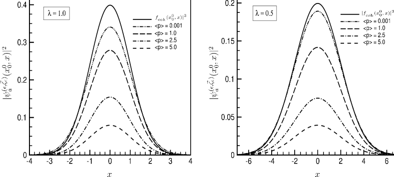
Figure 5: Plots of $|f_{{}_{\rm coh}}(\epsilon;x^{0}_{0},x)|^{2}$ and $|\psi_{a}^{(\epsilon,\vec{\zeta}_{\epsilon})}(x^{0}_{0},x)|^{2}$ for various $\lambda$ and momentum expectation values $\langle{\rm p}\rangle$: $|f_{{}_{\rm coh}}(\epsilon;x^{0}_{0},x)|^{2}$ represents the nonrelativistic probability density. For small values of the momentum expectation value $|\psi_{a}^{(\epsilon,\vec{\zeta}_{\epsilon})}(x^{0}_{0},x)|^{2}$ tends to $|f_{{}_{\rm coh}}(\epsilon;x^{0}_{0},x)|^{2}$. Here we have set $\kappa(1+\epsilon a)=1$.

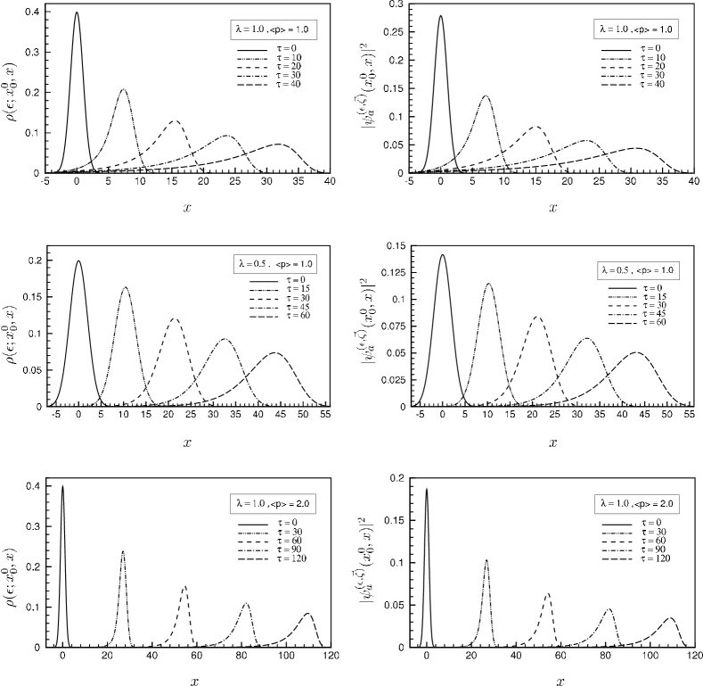
Figure 6: Graphs showing the time-evolution of the probability density $\rho(\epsilon;x^{0},x)$ and $|\psi_{a}^{(\epsilon,\vec{\zeta}_{\epsilon})}(x^{0},x)|^{2}$ for various values of $\lambda$, initial $\langle{\rm p}\rangle$, and $\epsilon=+1$: They spread with time $\tau$ while their maximum value decreases. The packets with smaller width spread faster confirming the behavior displayed in Figs. (2) and (3). The faster moving packets behave more like a classical particle. Unlike for a nonrelativistic coherent wave packet, the maximum of the probability density does not move with either of the velocity of the corresponding classical particle or the velocity expectation value of the packet. It moves with a higher velocity which is nevertheless smaller than $c$. For a quantitative analysis see footnote 7. Here we have set $\kappa(1+\epsilon a)=1$.

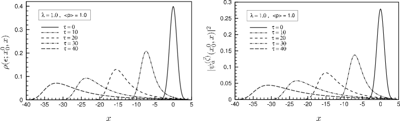
Figure 7: Graphs showing the time-evolution of the probability density $|\rho(\epsilon;x^{0},x)|^{2}$ and $|\psi_{a}^{(\epsilon,\vec{\zeta}_{\epsilon})}(x^{0},x)|^{2}$ for $\epsilon=-1$ and a positive initial momentum $\langle{\rm p}\rangle=1.0$: The probability density and the coherent KG wave function evolve in $-x^{0}$ direction. Here we have set $\kappa(1+\epsilon a)=1$.

Figs. 5 – 7 show the graphs of the $(1+1)$-dimensional analogs of $|\psi_{a}^{(\epsilon,\vec{\zeta}_{\epsilon})}(x)|^{2}$.

Since $\psi_{a}^{(\epsilon,\vec{\zeta}_{\epsilon})}$ is related by a unitary transformation to $|\vec{\zeta}_{\epsilon},\epsilon\rangle$, they share the properties of nonorthogonality, normalizability, and over-completeness. We can use $\psi_{a}^{(\epsilon,\vec{\zeta}_{\epsilon})}$ to yield a coherent state representation of arbitrary KG fields $\psi\in{\cal H}_{a}$:

$$\psi=\sum_{\epsilon=\pm}\int\frac{d^{2}\zeta_{\epsilon}}{\pi}\,g(\vec{\zeta}_{\epsilon},\epsilon)\,\psi_{a}^{(\epsilon,\vec{\zeta}_{\epsilon})},$$

where the wave function associated with $\psi$ in coherent state representation is defined by $g(\vec{\zeta}_{\epsilon},\epsilon):=\,(\psi_{a}^{(\epsilon,\vec{\zeta}_{\epsilon})},\psi)_{a}$.

3 Coherent States of a Free Charged Scalar Field in
$(1+1)$-Dimensions

In this section we examine the coherent KG fields in $(1+1)$-dimensions in more detail. For brevity of notation we will use the following scaled coherent state variable

$$\eta_{\epsilon}=\sqrt{\frac{2\hbar}{k}}\,\zeta_{\epsilon}=\alpha_{\epsilon}+i\beta_{\epsilon},$$ (34)

where $\alpha_{\epsilon}:=\Re(\eta_{\epsilon})$ and $\beta_{\epsilon}:=\Im(\eta_{\epsilon})$ have the dimension of length.

We recall that the coherent state wave function $f_{{}_{\rm coh}}(\epsilon,x)$ may be identified with the following normalized solution of (22), [31, 32].

$$f_{{}_{\rm coh}}(\epsilon,x)=\left[\frac{k}{\pi\hbar}\right]^{1/4}\!\!\!e^{-i\frac{k}{2\hbar}\alpha_{\epsilon}\beta_{\epsilon}}\,e^{i\frac{k\beta_{\epsilon}}{\hbar}x}\,e^{-\frac{k}{2\hbar}(x-\alpha_{\epsilon})^{2}}.$$ (35)

The Fourier transform of $f_{{}_{\rm coh}}(\epsilon,x)$ yields the corresponding coherent state wave function in the momentum representation (25),

$$f_{{}_{\rm coh}}(\epsilon,p)=\left[\frac{1}{\pi\hbar k}\right]^{1/4}\!\!\!e^{i\frac{k}{2\hbar}\alpha_{\epsilon}\beta_{\epsilon}}\,e^{-i\frac{\alpha_{\epsilon}}{\hbar}p}\,e^{-\frac{1}{2\hbar k}(p-k\beta_{\epsilon})^{2}}.$$ (36)

We obtain the coherent KG fields by substituting (36) in the $(1+1)$-dimensional analog of (33). This yields

$$\psi_{a}^{(\epsilon,\vec{\zeta}_{\epsilon})}(x^{0},x)=f_{{}_{\rm coh}}(\epsilon,x)\sqrt{\frac{\mbox{\scriptsize${\cal M}$}\hbar}{\kappa(1+\epsilon a)(2\pi\hbar k)}}\int_{\mathbb{R}}dp\,\frac{e^{-i\epsilon(\frac{x^{0}-x^{0}_{0}}{\hbar})\sqrt{\vec{p}^{2}+m^{2}c^{2}}}e^{-\frac{1}{2\hbar k}\,[p-k\beta_{\epsilon}-ik(x-\alpha_{\epsilon})]^{2}}}{[p^{2}+(mc)^{2}]^{1/4}}.$$ (37)

One can check that the nonrelativistic limit of $\psi_{a}^{(\epsilon,\vec{\zeta}_{\epsilon})}(x^{0}_{0},x)$ is the nonrelativistic coherent wave function $f_{{}_{\rm coh}}(\epsilon,x)$.

3.1 Observables, Uncertainty Relations, and the Classical Limit

In order to examine the physical properties of the coherent states constructed above we compute the expectation values of the basic observables in a coherent state and compare the result with the corresponding classical quantities. We also derive the associated minimum uncertainty relations and study their time-evolution and their nonrelativistic limit.

It is well-known that the physical quantities such as transition amplitudes and expectation values of observables are independent of the choice of representation of the quantum system [30, 26]. For example consider the observables $O^{\prime}:{\cal H}^{\prime}\rightarrow{\cal H}^{\prime}$ and $O_{a}=U_{a}^{-1}O^{\prime}U_{a}:{\cal H}_{a}\rightarrow{\cal H}_{a}$ which are respectively associated with the Foldy representation and the one-component representation. Then,

$$\langle O_{a}\rangle_{\epsilon}:=(\psi_{a}^{(\epsilon,\vec{\zeta}_{\epsilon})},\,O_{a}\,\psi_{a}^{(\epsilon,\vec{\zeta}_{\epsilon})})_{a}=\langle\vec{\zeta}_{\epsilon},\epsilon|O^{\prime}|\vec{\zeta}_{\epsilon},\epsilon\rangle=:\langle\,O^{\prime}\rangle_{\epsilon},$$ (38)

where we have used (16). In computing expectation values we will make use of these relations and the following formulas that follow from (35) and (36).

$$\langle r(X^{\prime})\rangle_{\epsilon} \!\!\!\!=\!\!\!\! \sqrt{\frac{k}{\pi\hbar}}\,\int_{\mathbb{R}}dx\,r(x)\,e^{-\frac{k}{\hbar}(x-\alpha_{\epsilon})^{2}},$$ (39)

$$\langle s(P^{\prime})\rangle_{\epsilon} \!\!\!\!=\!\!\!\! \frac{1}{\sqrt{\pi\hbar k}}\,\int_{\mathbb{R}}dp\,s(p)\,e^{-\frac{1}{\hbar k}(p-k\beta_{\epsilon})^{2}},$$ (40)

$$\langle s({\rm p})\sigma_{3}\rangle_{\epsilon} \!\!\!\!=\!\!\!\! \frac{\epsilon}{\sqrt{\pi\hbar k}}\,\int_{\mathbb{R}}dp\,s(p)\,e^{-\frac{1}{\hbar k}(p-k\beta_{\epsilon})^{2}},$$ (41)

where $r$ and $s$ are arbitrary functions rendering the integrals in (39) – (41) convergent.

To explore the ‘coherence’ behavior of the solution given in Eq. (35) we first examine the minimum uncertainty relationship. In view of (39) and (40), we can easily show that

$$\langle X\rangle_{\epsilon} \!\!\!\!=\!\!\!\! \langle X^{\prime}\rangle_{\epsilon}=\alpha_{\epsilon}\,,~{}~{}~{}~{}~{}~{}~{}~{}~{}~{}~{}~{}~{}~{}\langle X^{2}\rangle_{\epsilon}=\langle X^{\prime 2}\rangle_{\epsilon}=\alpha_{\epsilon}^{2}+\frac{\hbar}{2k}\,,$$ (42)

$$\langle P\rangle_{\epsilon} \!\!\!\!=\!\!\!\! \langle P^{\prime}\rangle_{\epsilon}=k\,\beta_{\epsilon}\,,~{}~{}~{}~{}~{}~{}~{}~{}~{}~{}~{}~{}\langle P^{2}\rangle_{\epsilon}=\langle P^{\prime 2}\rangle_{\epsilon}=k^{2}\,\beta_{\epsilon}^{2}+\frac{\hbar k}{2},$$ (43)

where $\alpha_{\epsilon}$ and $\beta_{\epsilon}$ are introduced in (34). In view of (42) and (43), we have the following dispersions for position and momentum operators, respectively.

$$(\Delta X)_{\epsilon}^{2} \!\!\!\!=\!\!\!\! (\Delta X^{\prime})_{\epsilon}^{2}:=\langle X^{\prime 2}\rangle_{\epsilon}-\langle X^{\prime}\rangle_{\epsilon}^{2}=\frac{\hbar}{2k}\,,$$ (44)

$$(\Delta P)_{\epsilon}^{2} \!\!\!\!=\!\!\!\! (\Delta P^{\prime})_{\epsilon}^{2}:=\langle P^{\prime 2}\rangle_{\epsilon}-\langle P^{\prime}\rangle_{\epsilon}^{2}=\frac{\hbar k}{2}\,.$$ (45)

Hence, as expected, $(\Delta X)_{\epsilon}(\Delta P)_{\epsilon}=(\Delta X^{\prime})_{\epsilon}(\Delta P^{\prime})_{\epsilon}=\hbar/2$, i.e., the minimum uncertainty relation is realized by the initial coherent state (at $x^{0}=x^{0}_{0}$).

Next, we examine the effect of time-evolution on the minimum uncertainty relation. The evolution of the operators $X^{\prime}$ and $P^{\prime}$ in the Heisenberg picture are determined by

$$\frac{dX^{\prime}}{dx^{0}}=\frac{1}{i\hbar}\,[X^{\prime},H^{\prime}]=\frac{{\rm p}}{\sqrt{{\rm p}^{2}+m^{2}c^{2}}}\,\sigma_{3}\,,~{}~{}~{}~{}~{}~{}~{}~{}\frac{dP^{\prime}}{dx^{0}}=\frac{1}{i\hbar}\,[P^{\prime},H^{\prime}]=0\,.$$ (46)

The Heisenberg operators $X^{\prime}(x^{0})$ and $P^{\prime}(x^{0})$ are therefore given by

$$X^{\prime}(x^{0})=X^{\prime}+\frac{x^{0}\,{\rm p}}{\sqrt{{\rm p}^{2}+m^{2}c^{2}}}\,\sigma_{3}\,,~{}~{}~{}~{}~{}~{}~{}~{}~{}~{}~{}~{}~{}P^{\prime}(x^{0})=P^{\prime}.$$ (47)

Using (46), (47) and (41) and doing the necessary calculations, we have

$$\langle X^{\prime}(x^{0})\rangle_{\epsilon} = \langle X^{\prime}\rangle_{\epsilon}+\langle\frac{dX^{\prime}}{dx^{0}}\rangle_{\epsilon}\,x^{0}\,,$$ (48)

$$\langle\dot{X}^{\prime}\rangle_{\epsilon} = \langle\frac{dX^{\prime}}{dx^{0}}\rangle_{\epsilon}=\frac{\epsilon}{\sqrt{\pi\hbar k}}\,\int_{\mathbb{R}}dp\,\frac{{\rm p}}{\sqrt{{\rm p}^{2}+m^{2}c^{2}}}\,e^{-\frac{1}{\hbar k}(p-k\beta_{\epsilon})^{2}},$$ (49)

$$\langle X^{\prime}(x^{0})^{2}\rangle_{\epsilon} = \langle X^{\prime 2}\rangle_{\epsilon}+2\alpha_{\epsilon}\langle\dot{X}^{\prime}\rangle_{\epsilon}\,x^{0}+\langle\dot{X}^{\prime 2}\rangle_{\epsilon}\,x^{0\,2},$$ (50)

$$\langle\dot{X}^{\prime 2}\rangle_{\epsilon} = \langle\left(\frac{dX^{\prime}}{dx^{0}}\right)^{2}\rangle_{\epsilon}=\frac{1}{\sqrt{\pi\hbar k}}\,\int_{\mathbb{R}}dp\,\frac{p^{2}}{p^{2}+m^{2}c^{2}}\,e^{-\frac{1}{\hbar k}(p-k\beta_{\epsilon})^{2}}.$$ (51)

Now, we employ (48) and (50) to compute the dispersion of the position operator $X^{\prime}(x^{0})$ in the coherent state:

$$(\Delta X^{\prime}(x^{0}))_{\epsilon}^{2}=\frac{\hbar}{2k}+(\Delta\dot{X}^{\prime})_{\epsilon}^{2}\,x^{0\,2},$$ (52)

where $(\Delta\dot{X}^{\prime})_{\epsilon}^{2}:=\langle\dot{X}^{\prime 2}\rangle_{\epsilon}-\langle\dot{X}^{\prime}\rangle_{\epsilon}^{2}$. Since $P^{\prime}$ is conserved, the dispersion $(\Delta P^{\prime})_{\epsilon}$ does not change in time, and for all $x^{0}\in\mathbb{R}$

$$(\Delta X(x^{0}))_{\epsilon}(\Delta P(x^{0}))_{\epsilon}=(\Delta X^{\prime}(x^{0}))_{\epsilon}(\Delta P^{\prime}(x^{0}))_{\epsilon}=\frac{\hbar}{2}\sqrt{1+\frac{2k}{\hbar}\,(\Delta\dot{X}^{\prime})_{\epsilon}^{2}\,x^{0\,2}}.$$ (53)

The integrals in (37), (49) and (51) cannot be evaluated analytically, and we could not obtain the explicit form of $\psi_{a}^{(\epsilon,\vec{\zeta}_{\epsilon})}(x^{0}_{0},x)$, $\langle\dot{X}^{\prime}\rangle_{\epsilon}$, $\langle\dot{X}^{\prime 2}\rangle_{\epsilon}$ and $(\Delta\dot{X}^{\prime})_{\epsilon}^{2}$. We have instead calculated them numerically and plotted their graphs as functions of the expectation value of momentum ($k\beta_{\epsilon}$), time, and other relevant parameters. To describe the behavior of these quantities, it is convenient to introduce the dimensionless parameter $\lambda:=\sqrt{2\hbar k}/(mc)$ and express the relevant relations in dimensionless units, i.e., the units where the momentum, position, energy and time are respectively measured in units of $mc$, $\lambda_{c}=\hbar/(mc)$ (the Compton wavelength), $mc^{2}$ and $\lambda_{c}/c=\hbar/(mc^{2})$. Note that in our notation the quantity $\dot{X}=\frac{dX}{cdt}$ is dimensionless, so the velocity is measured in units of $c$.

The dimensionless parameter $\lambda$ is just the ratio of the Compton wavelength and the characteristic oscillator length $\sigma:=\sqrt{\hbar/(2k)}$, i.e., $\lambda:=\lambda_{c}/\sigma$. In view of (44), $\sigma$ determines the width of the wave packet, and $\lambda^{-1}$ is a measure of the localization of the wave packet. It is usually argued that a relativistic particle cannot be localized more accurately than the Compton wavelength, for otherwise pair production occurs for $E>2mc^{2}$, [27]. This situation restricts the range of allowed values of $\lambda$. If we rewrite (44) in dimensionless unit, we find that the condition $\Delta X\geq\lambda_{c}$ implies $\lambda\leqslant 1$. We will see from our plots that the smaller the value of $\lambda$ becomes the more classical the coherent state behaves.

Expressing $\langle\dot{X}^{\prime}\rangle_{\epsilon}$, $\langle\dot{X}^{\prime 2}\rangle_{\epsilon}$, $\langle X^{\prime}(x^{0})\rangle_{\epsilon}$, $(\Delta X^{\prime}(x^{0}))_{\epsilon}^{2}$ and $(\Delta X(x^{0}))_{\epsilon}(\Delta P(x^{0}))_{\epsilon}$ in dimensionless units yields

$$\langle\dot{X}^{\prime}\rangle_{\epsilon} \!\!\!\!=\!\!\!\! \frac{\epsilon}{\lambda}\,\sqrt{\frac{2}{\pi}}\,\int_{\mathbb{R}}dp\,\frac{{\rm p}}{\sqrt{1+{\rm p}^{2}}}\,e^{-\frac{2}{\lambda^{2}}(p-k\beta_{\epsilon})^{2}},$$ (54)

$$\langle\dot{X}^{\prime 2}\rangle_{\epsilon} \!\!\!\!=\!\!\!\! \frac{1}{\lambda}\,\sqrt{\frac{2}{\pi}}\,\int_{\mathbb{R}}dp\,\frac{{\rm p}^{2}}{1+{\rm p}^{2}}\,e^{-\frac{2}{\lambda^{2}}(p-k\beta_{\epsilon})^{2}},$$ (55)

$$\langle X^{\prime}(\tau)\rangle_{\epsilon} \!\!\!\!=\!\!\!\! \langle X^{\prime}\rangle_{\epsilon}+\langle\dot{X}^{\prime}\rangle_{\epsilon}\,\tau\,,$$ (56)

$$(\Delta X^{\prime}(\tau))_{\epsilon} \!\!\!\!=\!\!\!\! (\Delta X(\tau))_{\epsilon}=\frac{1}{\lambda}\sqrt{1+\lambda^{2}(\Delta\dot{X}^{\prime})^{2}_{\epsilon}\,\tau^{2}}\,,$$ (57)

$$(\Delta X(\tau))_{\epsilon}(\Delta P(\tau))_{\epsilon} \!\!\!\!=\!\!\!\! (\Delta X^{\prime}(\tau))_{\epsilon}(\Delta P^{\prime}(\tau))_{\epsilon}=\frac{1}{2}\sqrt{1+\lambda^{2}(\Delta\dot{X}^{\prime})^{2}_{\epsilon}\,\tau^{2}}\,,$$ (58)

where $\tau:=x^{0}/\lambda_{c}=ct/\lambda_{c}$ is a dimensionless time parameter. The nonrelativistic quantum mechanical analogs of (54) – (58) have the form

$$\langle\dot{\rm x}\rangle_{\rm nr} \!\!\!\!=\!\!\!\! k\beta=\langle{\rm p}\rangle,~{}~{}~{}~{}~{}~{}\langle\dot{\rm x}^{2}\rangle_{\rm nr}=\frac{\lambda^{2}}{4}+\langle{\rm p}\rangle^{2},~{}~{}~{}~{}~{}~{}\langle{\rm x}(\tau)\rangle_{\rm nr}=\langle{\rm x}\rangle+\langle{\rm p}\rangle\,\tau\,,$$ (59)

$$\Delta{\rm x}(\tau) \!\!\!\!=\!\!\!\! \frac{1}{\lambda}\sqrt{1+\frac{1}{4}\lambda^{4}\tau^{2}}\,,~{}~{}~{}~{}~{}~{}\Delta{\rm x}(\tau)\Delta{\rm p}(\tau)=\frac{1}{2}\sqrt{1+\frac{1}{4}\lambda^{4}\tau^{2}}\,.$$ (60)

Now, we are in a position to plot these quantities and perform a relativistic-to-nonrelativistic and quantum-to-classical comparisons.

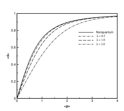
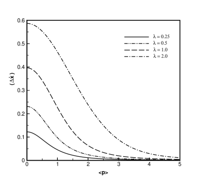
Figure 1: Graphs of the velocity expectation value $\langle\dot{\rm x}\rangle$ (left) and the dispersion $(\Delta\dot{\rm x})$ (right) as functions of the momentum expectation value $\langle{\rm p}\rangle$ for coherent states of a free particle with different values of $\lambda$ and the corresponding classical (nonquantum) curve: Momentum and velocity are given in units of $mc$ and $c$, respectively. For small values of $\lambda$ the quantum curves tend to the classical curve. The dispersion in velocity decreases as the velocity increases.

Fig. 1 shows the dependence of the velocity expectation value $\langle\dot{\rm x}\rangle$ and dispersion in velocity $\Delta\dot{\rm x}$ on momentum expectation value $\langle{\rm p}\rangle$ for different values of $\lambda$. It also includes the graph of the corresponding classical curve, i.e., $\langle\dot{\rm x}\rangle=\frac{\langle{\rm p}\rangle}{\sqrt{1+\langle{\rm p}\rangle^{2}}}$. As one reduces the value of $\lambda$, the quantum curve tends to the classical curve. Moreover, for higher velocities the dispersion in velocity is small, and as we shall argue below, the spreading of the wave packet is slower. Similarly, the dispersion in position (the width of the coherent wave packet), the product of the position and momentum dispersions, and consequently the minimum uncertainty relation are velocity-dependent. This is a feature of the relativistic coherent states that does not survive the nonrelativistic limit; in nonrelativistic QM these quantities are velocity-independent.

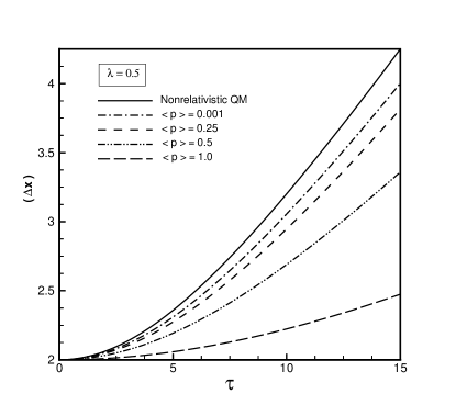
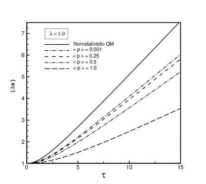
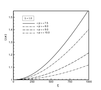
Figure 2: Plots of the dispersion in position $\Delta{\rm x}$ as a function of time for various $\lambda$ and momentum expectation values $\langle{\rm p}\rangle$: The nonrelativistic dispersion which turns out to be larger than the relativistic dispersion is also depicted. The higher $\langle{\rm p}\rangle$ becomes the smaller $\Delta{\rm x}$ is.

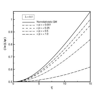
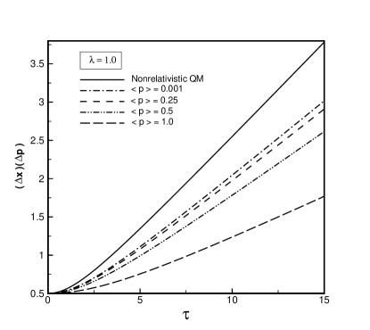
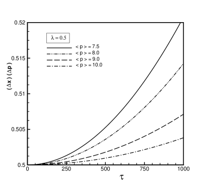
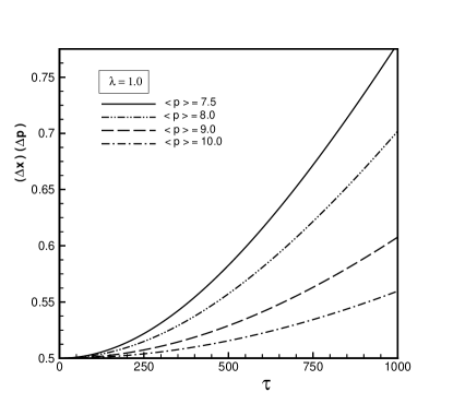
Figure 3: Plots of $(\Delta{\rm x})(\Delta{\rm p})$ in terms of time for various $\lambda$ and momentum expectation values $\langle{\rm p}\rangle$: Nonrelativistic QM yields a larger value for $(\Delta{\rm x})(\Delta{\rm p})$ than the relativistic QM. The higher the momentum becomes the smaller $(\Delta{\rm x})(\Delta{\rm p})$ gets. The packets with smaller width (larger $\lambda$) yield larger values for $(\Delta{\rm x})(\Delta{\rm p})$.

Fig. 2 shows the dispersion in position as a function of time for various values of the momentum expectation value and the parameter $\lambda$. It also shows the corresponding nonrelativistic quantum mechanical dispersion. The relativistic dispersion turns out to be smaller than the nonrelativistic dispersion. Also as one increases the momentum the uncertainty in position decreases. In view of the fact that the momentum operator does not depend on time, this shows that the product of the position and momentum dispersions is smaller for the faster moving packets. See Figs. 3 which also show that the spreading of a faster moving coherent wave packet has a smaller rate than that of the slower moving packets. We will arrive at the same conclusion when we consider the graphs of the evolution of the probability density below.

Next, we explore the behavior of the energy expectation value. Recall that in the Foldy representation the Hamiltonian operator is given by $H^{\prime}=\sqrt{{\rm p}^{2}+m^{2}c^{2}}\,\sigma_{3}$. Hence, we define the energy operator according to

$$E^{\prime}:=c\,{\cal C}^{\prime}H^{\prime}=\sqrt{c^{2}{\rm p}^{2}+m^{2}c^{4}}\,\sigma_{0}\,.$$ (61)

In view of (41), its expectation value is given in dimensionless units by

$$\langle E\rangle_{\epsilon}:=\langle E^{\prime}\rangle_{\epsilon}=\langle\sqrt{c^{2}{\rm p}^{2}+m^{2}c^{4}}\rangle_{\epsilon}=\frac{1}{\lambda}\,\sqrt{\frac{2}{\pi}}\,\int_{\mathbb{R}}dp\,\sqrt{1+{\rm p}^{2}}\,e^{-\frac{2}{\lambda^{2}}(p-k\beta_{\epsilon})^{2}}.$$ (62)

We can also compare it with its nonrelativistic counterpart, namely

$$\langle E\rangle_{\rm nr}=1+\langle\frac{{\rm p}^{2}}{2}\rangle=1+\frac{1}{\lambda}\,\sqrt{\frac{2}{\pi}}\,\int_{\mathbb{R}}dp\,{\rm p}^{2}\,e^{-\frac{2}{\lambda^{2}}(p-k\beta_{\epsilon})^{2}}=1+\frac{\lambda^{2}}{8}+\frac{\langle{\rm p}\rangle^{2}}{2}.$$ (63)

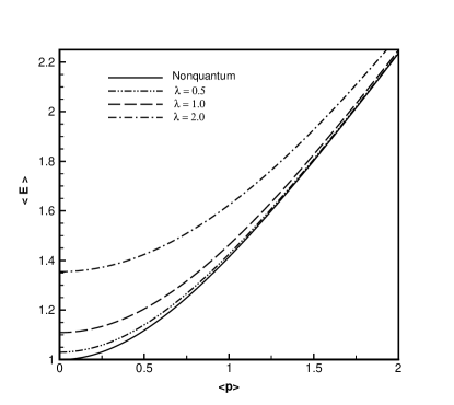
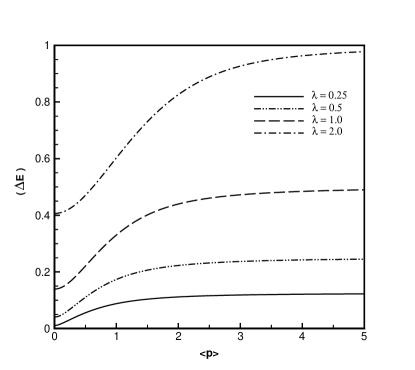
Figure 4: Graphs of the energy expectation value $\langle E\rangle$ (left) and its dispersion $(\Delta E)$ (right) as functions of the momentum expectation value $\langle{\rm p}\rangle$ for the coherent states of a free particle with different $\lambda$: The graphs of the corresponding classical (nonquantum) and nonrelativistic (quantum) curves are also given. For small values of $\lambda$ the coherent state displays completely classical behavior.

In Fig. 4 we plot the expectation value of energy and its dispersion $\Delta E$ in terms of the momentum expectation value for different $\lambda$ and the corresponding classical (nonquantum) and nonrelativistic (quantum mechanical) curves. From these graphs we can see that for small values of $\lambda$ the coherent states display completely classical behavior. Table 1 shows some typical relativistic and nonrelativistic energy expectation values for small momentum and various values of $\lambda$. The relativistic expectation value of energy is smaller than its nonrelativistic counterpart and closer to the classical relativistic energy. For small values of $\lambda$ the relativistic and nonrelativistic energy expectation values coincide and tend to the classical result.

$\langle{\rm p}\rangle$		$0.1$			$0.001$
$\lambda$	$0.25$	$0.5$	$2.0$	$0.25$	$0.5$	$2.0$
$\langle E\rangle/E_{\rm cl.}$	$1.00758$	$1.02944$	$1.35062$	$1.00772$	$1.02997$	$1.35453$
$\langle E\rangle_{\rm nr}/E_{\rm cl.}$	$1.00777$	$1.03109$	$1.49751$	$1.00781$	$1.03125$	$1.50000$

Table 1: Comparison of the relativistic and nonrelativistic energy expectation values for small momenta. The relativistic expectation value is smaller than the nonrelativistic expectation value and closer to the classical relativistic energy. For small values of $\lambda$ the relativistic and nonrelativistic energy expectation values coincide and tend to the classical result.

3.2 Probability Density and Its Time-Evolution

The probability density $\rho(x^{0},x)$ for a coherent state with definite charge parity $\epsilon$, in dimensionless units, has the form

$$\rho(\epsilon;x^{0},x):=|f_{{}_{\rm coh}}(\epsilon;x^{0},x)|^{2}=\frac{1}{\lambda\pi\sqrt{2\pi}}\left[S^{2}+T^{2}\right],$$ (64)

where we have made use of Eqs. (I-63), (30), (31), (35) and introduced

$$S \!\!\!\!:=\!\!\!\! \int_{\mathbb{R}}dp\,e^{-\frac{1}{\lambda^{2}}(p-k\beta_{\epsilon})^{2}}\,\cos{\left[p(x-\alpha_{\epsilon})-\epsilon\tau\sqrt{1+p^{2}}\right]},$$ (65)

$$T \!\!\!\!:=\!\!\!\! \int_{\mathbb{R}}dp\,e^{-\frac{1}{\lambda^{2}}(p-k\beta_{\epsilon})^{2}}\,\sin{\left[p(x-\alpha_{\epsilon})-\epsilon\tau\sqrt{1+p^{2}}\right]}.$$ (66)

Evaluating these integrals or using Eq. (35) yields

$$\rho(\epsilon;x^{0}_{0},x)=|f_{{}_{\rm coh}}(\epsilon;x^{0}_{0},x)|^{2}=\frac{\lambda}{\sqrt{2\pi}}\,e^{-\frac{\lambda^{2}}{2}(x-\alpha_{\epsilon})^{2}}.$$ (67)

Therefore, the probability density at time $x^{0}_{0}$ is just the nonrelativistic Schrödinger probability density and does not depend on the particle’s momentum. But at later times, the probability density depends on the particle’s momentum $\langle{\rm p}\rangle_{\epsilon}=k\beta_{\epsilon}$. Also, from these equations we see that for $\tau\neq 0$ the probability density depends on $\epsilon$, hence its evolution differs for positive and negative charges. The difference is that the packets with negative charge parity move backward in time. This means that the physical momentum is to be identified with $\epsilon\,{\rm p}$, [35]. Figs. 5 – 7 show plots of $\rho(\epsilon;x^{0},x)$.

Eq. (37) gives an expression for the coherent KG field, $\psi_{a}^{(\epsilon,\vec{\zeta}_{\epsilon})}$, in $(1+1)$-dimensions. In order to compare this expression with that of its nonrelativistic analog, namely $f_{{}_{\rm coh}}(\epsilon;x^{0},x)$, we plot them in terms of the momentum expectation value for various values of the parameter $\lambda$. First, we rewrite (37) in dimensionless units and compute

$$|\psi_{a}^{(\epsilon,\vec{\zeta}_{\epsilon})}(x^{0},x)|^{2}=\frac{1}{\lambda\pi\kappa(1+\epsilon a)\sqrt{2\pi}}\left[U^{2}+V^{2}\right],$$ (68)

where

$$U \!\!\!\!:=\!\!\!\! \int_{\mathbb{R}}dp\,\frac{e^{-\frac{1}{\lambda^{2}}(p-k\beta_{\epsilon})^{2}}}{[1+p^{2}]^{\frac{1}{4}}}\,\cos{\left[p(x-\alpha_{\epsilon})-\epsilon\tau\sqrt{1+p^{2}}\right]},$$

$$V \!\!\!\!:=\!\!\!\! \int_{\mathbb{R}}dp\,\frac{e^{-\frac{1}{\lambda^{2}}(p+k\beta_{\epsilon})^{2}}}{[1+p^{2}]^{\frac{1}{4}}}\,\sin{\left[p(x-\alpha_{\epsilon})-\epsilon\tau\sqrt{1+p^{2}}\right]}.$$

In the nonrelativistic limit, $U$ and $V$ respectively tend to $S$ and $T$. This means that the nonrelativistic limit of $|\psi_{a}^{(\epsilon,\vec{\zeta}_{\epsilon})}(x^{0},x)|^{2}$ coincides with the nonrelativistic probability density $|f_{{}_{\rm coh}}(\epsilon;x^{0},x)|^{2}$ for all $x^{0}\in\mathbb{R}$.

Fig. 5 gives the plots of $|f_{{}_{\rm coh}}(\epsilon;x^{0}_{0},x)|^{2}$ and $|\psi_{a}^{(\epsilon,\vec{\zeta}_{\epsilon})}(x^{0}_{0},x)|^{2}$ for various values of the momentum expectation value, $\langle p\rangle_{\epsilon}=k\beta_{\epsilon}$, and $\lambda$. As seen from this figure, $|\psi_{a}^{(\epsilon,\vec{\zeta}_{\epsilon})}(x^{0}_{0},x)|^{2}$ depends on the particle’s initial momentum expectation value. For small values of the latter $|\psi_{a}^{(\epsilon,\vec{\zeta}_{\epsilon})}(x^{0}_{0},x)|^{2}$ tends to $|f_{{}_{\rm coh}}(\epsilon;x^{0}_{0},x)|^{2}$.

Fig. 6 shows that both the probability density $\rho(\epsilon;x^{0},x)$ and modulus-square $|\psi_{a}^{(\epsilon,\vec{\zeta}_{\epsilon})}(x^{0},x)|^{2}$ of a coherent KG wave packet spread with time while their maximum value decreases. The nature of this spreading depends on the momentum expectation value and the initial width of the wave packet. The more localized the initial coherent packet is (the closer $\lambda$ gets to one) the faster it spreads. This is in complete accordance with Figs. 2 and 3. Also, the fast moving packets behave more like a classical particle; they travel a larger distance without noticeable spreading.

The spreading of the relativistic coherent wave packet is similar to the one encountered in nonrelativistic QM [34]. However, unlike for a nonrelativistic coherent wave packet, the maximum of the probability density $\rho(\epsilon;x^{0},x)$ and the modulus-square $|\psi_{a}^{(\epsilon,\vec{\zeta}_{\epsilon})}(x^{0},x)|^{2}$ of a relativistic coherent wave packet do not move with its velocity expectation value or the velocity of the corresponding classical particle. They move with a higher velocity which is nevertheless smaller than the velocity of light. This is easily seen from the graphs given in Fig. 6.

Fig. 7 shows the time-evolution of the probability density and $|\psi_{a}^{(\epsilon,\vec{\zeta}_{\epsilon})}(x^{0}_{0},x)|^{2}$ for $\epsilon=-1$ and a positive initial momentum expectation value. As demonstrated by this graph, the probability density and the KG wave function evolve in $-x^{0}$ direction (in contrast to Fig. 6).

4 Coherent States of a Free Neutral Field

Neutral scalar particles are described by real KG fields which we briefly studied in [12]. As we showed there, a characteristic feature of a real KG field is that its position wave function $f(\epsilon,\vec{x})$ satisfies $f(\epsilon,\vec{x})=f(-\epsilon,\vec{x})^{*}$. This condition together with (35) restrict the parameters $\beta_{\epsilon}$ and $\alpha_{\epsilon}$ of the coherent states according to

$$\beta_{-\epsilon}=-\beta_{\epsilon},~{}~{}~{}~{}~{}~{}~{}~{}~{}~{}\alpha_{-\epsilon}=\alpha_{\epsilon}.$$ (69)

In the one-component representation, the coherent states for neutral field is defined by

$$\psi_{a}^{(\vec{\zeta})}:=\frac{1}{\sqrt{2}}\left[\psi_{a}^{(+,\vec{\zeta})}+\psi_{a}^{(-,\vec{\zeta}^{*})}\right],$$ (70)

where the coherent wave functions $f_{{}_{\rm coh}}(+,\vec{x})$ and $f_{{}_{\rm coh}}(-,\vec{x})$ are given by (35) and (69).

As seen from Fig. 7 the coherent wave packet with negative charge parity moves backward in time. Therefore, the physical momentum for states with charge parity $\epsilon$ is $\epsilon\vec{\rm p}$, [35]. Hence, the physical momentum operator for a general KG field may be identified with ${\cal C}\vec{\rm p}$. Using this expression in computing the expectation values, probability densities, etc., we have found that all the results and graphs of the preceding section are valid for a free neutral particle.

5 Coupling to a Uniform Magnetic Field

Consider a scalar charged particle with the electric charge $e$ in a constant homogeneous magnetic field directed along the (positive) $x^{3}$-axis, $\vec{B}=(0,0,B)$ with $B>0$. In the symmetric gauge the electromagnetic vector potential has the form

$$\vec{A}(\vec{x})=-\frac{1}{2}(\vec{x}\times\vec{B})~{}~{}\Rightarrow~{}~{}~{}~{}A_{0}=A_{3}=0,\hskip 14.22636ptA_{1}=-\frac{1}{2}Bx^{2},\hskip 14.22636ptA_{2}=\frac{1}{2}Bx^{1}$$ (71)

In order to fix the notation and compare the quantum mechanical and classical results, we first review the classical treatment of the problem.

5.1 Classical Treatment

The classical motion may be obtained using the classical Hamiltonian [36]

$$H_{\rm cl.}=E:=\sqrt{c^{2}\vec{\Pi}^{2}+m^{2}c^{4}},$$ (72)

where $E$ and $\vec{\Pi}$ stand for the particle’s energy and kinetic momentum, respectively. The latter is given, in the gauge (71), by

$$\vec{\Pi}=\vec{p}-e\vec{A}=\gamma m\vec{v},\hskip 21.33955pt\Pi_{1}=p_{1}+\frac{eB}{2}x^{2},\hskip 21.33955pt\Pi_{2}=p_{2}-\frac{eB}{2}x^{1},\hskip 21.33955pt\Pi_{3}=p_{3},$$ (73)

where $\vec{p}$ is the canonical momentum conjugate to the position $\vec{x}$ of the particle, $\vec{v}=(\dot{x}^{1},\dot{x}^{2},\dot{x}^{3})$ is the velocity, and $\gamma$ is the Lorentz factor. The Hamiltonian is a constant of motion, so the magnitude of the velocity does not change and $\gamma$ is a constant.

The Hamilton’s equations of motion read

$$\dot{\vec{x}} \!\!\!\!:=\!\!\!\! \frac{d\vec{x}}{dx^{0}}=\frac{\vec{\Pi}}{\sqrt{\vec{\Pi}^{2}+(mc)^{2}}}\,,$$ (74)

$$\dot{p}_{1} \!\!\!\!:=\!\!\!\! \frac{dp_{1}}{dx^{0}}=\frac{(\frac{eB}{2})\Pi_{2}}{\sqrt{\vec{\Pi}^{2}+(mc)^{2}}}\,,~{}~{}~{}~{}~{}~{}\dot{p}_{2}:=\frac{dp_{2}}{dx^{0}}=\frac{-(\frac{eB}{2})\Pi_{1}}{\sqrt{\vec{\Pi}^{2}+(mc)^{2}}}\,,~{}~{}~{}~{}~{}~{}\dot{p}_{3}:=\frac{dp_{3}}{dx^{0}}=0.$$ (75)

They are equivalent to [36]

$$\frac{d\vec{v}}{dx^{0}}=\vec{v}\times\vec{\omega}_{B},$$ (76)

where $\vec{\omega}_{B}$ is the gyration or precession frequency and has the form

$$\vec{\omega}_{B}:=\frac{e\vec{B}}{\gamma mc}=\frac{ec\vec{B}}{E}.$$ (77)

The motion described by (76) is a circular motion perpendicular to $\vec{B}$ and a uniform translational motion parallel to $\vec{B}$. The solution of (76) has the form [36]

$$\vec{v}(x^{0})=\dot{x}^{3}\hat{e}_{3}+R\omega_{B}(\hat{e}_{1}-i\hat{e}_{2})e^{-i\omega_{B}x^{0}},$$ (78)

where $R$ is the gyration radius, $\hat{e}_{i}$ is the unit vector along the $x^{i}$-axis, and the physical velocity of the particle is given by the real part of this equation. For a positive charge $e$, it represents a counterclockwise rotation when viewed in the direction of $\vec{B}$, [36]. Integrating (78) yields the position of the particle:

$$\vec{X}(x^{0})=\vec{X}_{\rm g.c.}+\dot{x}^{3}x^{0}\hat{e}_{3}+iR(\hat{e}_{1}-i\hat{e}_{2})e^{-i\omega_{B}x^{0}}.$$ (79)

The classical path is a helix with center $\vec{X}_{\rm g.c.}$, radius $R$, and pitch angle $\vartheta\!=\!\tan^{-1}({\rm p}_{3}/eBR)$.

In view of (74) and (75), the coordinates of the gyration center,

$$x^{1}_{\rm g.c.}:=\frac{x^{1}}{2}+\frac{p_{2}}{eB},~{}~{}~{}~{}~{}~{}~{}~{}~{}~{}~{}x^{2}_{\rm g.c.}:=\frac{x^{2}}{2}-\frac{p_{1}}{eB},$$ (80)

are constants of motion [37]. We can use them to express the gyration radius $R$ and the component $L_{3}$ of the angular momentum along the $x^{3}$-direction. This yields

$$R \!\!\!\!=\!\!\!\! \sqrt{(x^{1}-x^{1}_{\rm g.c.})^{2}+(x^{2}-x^{2}_{\rm g.c.})^{2}}=\frac{\Pi_{\perp}}{eB}\,$$ (81)

$$L_{3} \!\!\!\!=\!\!\!\! x^{1}p_{2}-x^{2}p_{1}=\frac{eB}{2}\left[(x^{1}_{\rm g.c.})^{2}+(x^{2}_{\rm g.c.})^{2}-R^{2}\right]=\frac{eB}{2}\left(R_{\rm g.c.}^{2}-R^{2}\right),$$ (82)

where $\Pi_{\perp}:=\sqrt{\Pi_{1}^{2}+\Pi_{2}^{2}}$. These relations are consistent with the fact that $\Pi_{3}$ and the total energy are also conserved quantities [36, 37].

5.2 Quantum Mechanical Treatment

In relativistic quantum mechanics, the charged scalar particle interacting with a constant homogeneous magnetic field may be described by the KG equation (1) where $D$ is given by

$$D=\hbar^{-2}[\vec{\Pi}^{2}+(mc)^{2}]=\hbar^{-2}[(\vec{\rm p}-e\vec{A})^{2}+(mc)^{2}],$$ (83)

and $\vec{A}$ is the vector potential (71).

In the Foldy representation, the Hamiltonian has the form

$$H^{\prime}=\sqrt{\vec{\Pi}^{2}+m^{2}c^{2}}\;\sigma_{3}=\sqrt{(\vec{\rm p}-e\vec{A})^{2}+m^{2}c^{2}}\;\sigma_{3}.$$ (84)

In the following we shall drop the symbol “$\otimes\,\sigma_{0}$” in (10) for simplicity, so that the position and momentum operators in the Foldy representation are identified with ordinary position and momentum operators acting in $L^{2}(\mathbb{R}^{3})$, i.e., $\vec{X}^{\prime}\equiv\vec{\rm x}$ and $\vec{P}^{\prime}\equiv\vec{\rm p}$. Using this convention, we may express the Heisenberg equations of motion in Foldy representation as

$$\dot{\vec{\rm x}}=\frac{d{\mbox{$\vec{\rm x}$}}}{dx^{0}}=\frac{1}{i\hbar}\left[{\mbox{$\vec{\rm x}$}},H^{\prime}\right]\,,~{}~{}~{}~{}~{}~{}~{}~{}~{}{\mbox{$\dot{\vec{\rm p}}$}}=\frac{d{\mbox{$\vec{\rm p}$}}}{dx^{0}}=\frac{1}{i\hbar}\left[{\mbox{$\vec{\rm p}$}},H^{\prime}\right]\,.$$ (85)

In contrast to the classical case, the commutators appearing in these equation do not admit a closed-form expression in terms of $\vec{\rm x}$ and $\vec{\rm p}$. This makes an explicit solution of (85) intractable. We have performed a first-order perturbative investigation of (85) and shown that similarly to the classical case the trajectory is a helix with constant gyration center and radius. We will not include the details of this investigation here. Rather we will present a nonperturbative numerical treatment of the problem that turns out to be more efficient for larger values of $\Lambda$ (respectively $B$).

In the Foldy-representation, the three-dimensional coherent state vectors are the tensor product of one-dimensional coherent state vectors $|\zeta^{i}_{\epsilon},\epsilon\rangle$ (with $i=1,2,3$) along the $x^{i}$-directions, i.e.,

$$|\vec{\zeta}_{\epsilon},\epsilon\rangle:=|\zeta^{1}_{\epsilon},\epsilon\rangle\otimes|\zeta^{2}_{\epsilon},\epsilon\rangle\otimes|\zeta^{3}_{\epsilon},\epsilon\rangle.$$ (86)

Because of the symmetry in $x^{1}$-$x^{2}$ plane, we take the width of the wave packet in $x^{1}$ and $x^{2}$ directions to be equal. The coherent state wave functions in the $x$- and $p$-representations are respectively given by

$$f_{{}_{\rm coh}}(\epsilon,\vec{x}) \!\!\!\!=\!\!\!\! f_{{}_{\rm coh}}(\epsilon,x^{1})f_{{}_{\rm coh}}(\epsilon,x^{2})f_{{}_{\rm coh}}(\epsilon,x^{3})$$ (87)

$$\!\!\!\!=\!\!\!\! \left[\frac{k_{\perp}^{2}k_{3}}{\pi^{3}\hbar^{3}}\right]^{1/4}e^{-i\frac{\vec{q}_{\epsilon}}{2\hbar}\cdot\vec{\alpha}_{\epsilon}}\,e^{i\frac{\vec{q}_{\epsilon}}{\hbar}\cdot\vec{x}}\,e^{-\frac{k_{\perp}}{2\hbar}(x^{1}-\alpha_{1\epsilon})^{2}}e^{-\frac{k_{\perp}}{2\hbar}(x^{2}-\alpha_{2\epsilon})^{2}}e^{-\frac{k_{3}}{2\hbar}(x^{3}-\alpha_{3\epsilon})^{2}},$$

$$f_{{}_{\rm coh}}(\epsilon,\vec{p}) \!\!\!\!=\!\!\!\! f_{{}_{\rm coh}}(\epsilon,p_{1})f_{{}_{\rm coh}}(\epsilon,p_{2})f_{{}_{\rm coh}}(\epsilon,p_{3})$$ (88)

$$\!\!\!\!=\!\!\!\! \left[\frac{1}{k_{\perp}^{2}k_{3}\pi^{3}\hbar^{3}}\right]^{1/4}e^{i\frac{\vec{q}_{\epsilon}}{2\hbar}\cdot\vec{\alpha}_{\epsilon}}\,e^{-i\frac{\vec{\alpha}_{\epsilon}}{\hbar}\cdot\vec{p}}\,e^{-\frac{1}{2\hbar k_{\perp}}(p_{1}-q_{1\epsilon})^{2}}e^{-\frac{1}{2\hbar k_{\perp}}(p_{2}-q_{2\epsilon})^{2}}e^{-\frac{1}{2\hbar k_{3}}(p_{3}-q_{3\epsilon})^{2}},$$

where $\vec{q}_{\epsilon}:=\sum_{i=1}^{3}k_{i}\beta_{i\epsilon}\hat{e}_{i}=\sum_{i=1}^{3}\langle{\rm p}_{i}\rangle_{\epsilon}\hat{e}_{i},~{}k_{\perp}\!:=\!k_{1}\!=\!k_{2}$, and we have made use of (35). The wave packet’s widths in $x^{1}$-$x^{2}$ and $x^{3}$ directions are respectively given by $\sigma_{\perp}=\sqrt{\hbar/(2k_{\perp})}$ and $\sigma_{3}=\sqrt{\hbar/(2k_{3})}$. Clearly (86) represents the minimum-uncertainty states.

Next, we consider a positive charged particle in such a coherent state and drop $\epsilon=+1$ for brevity. In order to compute the expectation value $\langle\vec{\zeta}|\vec{\rm x}(x^{0})|\vec{\zeta}\rangle$ (resp. $\langle\vec{\zeta}|\vec{\rm p}(x^{0})|\vec{\zeta}\rangle$) of the position (resp. momentum) operator at any given time $x^{0}$, we will use the following implicit solution of (85).

$${\rm x}^{i}(x^{0})=e^{i\frac{x^{0}}{\hbar}H^{\prime}}{\rm x}^{i}e^{-i\frac{x^{0}}{\hbar}H^{\prime}},~{}~{}~{}~{}~{}~{}~{}~{}~{}~{}{\rm p}_{i}(x^{0})=e^{i\frac{x^{0}}{\hbar}H^{\prime}}{\rm p}_{i}e^{-i\frac{x^{0}}{\hbar}H^{\prime}}.$$ (89)

We will also need to obtain the action of $H^{\prime}$ on the coherent state vector $|\vec{\zeta}\rangle$. Because of the square root appearing in (84) a direct calculation of $H^{\prime}|\vec{\zeta}\rangle$ encounters severe problems. We will avoid them by expressing the relevant quantities in an eigenbasis of

$$h^{\prime}:=H^{\prime 2}=(mc)^{2}+({\rm p}_{1}+\frac{eB}{2}{\rm x}^{2})^{2}+({\rm p}_{2}-\frac{eB}{2}{\rm x}^{1})^{2}+{\rm p}_{3}^{2}\,.$$ (90)

For example, for the expectation value of an operator $O(x^{0})$ in the coherent state vector $|\vec{\zeta}\rangle$, we have

$$\!\!\!\!\langle\vec{\zeta}|O(x^{0})|\vec{\zeta}\rangle \!\!\!\!=\!\!\!\! \langle\vec{\zeta}|e^{i\frac{x^{0}}{\hbar}\sqrt{h^{\prime}}}Oe^{-i\frac{x^{0}}{\hbar}\sqrt{h^{\prime}}}|\vec{\zeta}\rangle$$ (91)

$$\!\!\!\!=\!\!\!\! \sum_{n,\ell,n^{\prime},\ell^{\prime}}\int\!dk_{3}\!\!\int\!dk^{\prime}_{3}\,\langle\vec{\zeta}|e^{i\frac{x^{0}}{\hbar}\sqrt{h^{\prime}}}|n,\ell,k_{3}\rangle\langle n,\ell,k_{3}|O|n^{\prime},\ell^{\prime},k^{\prime}_{3}\rangle\langle n^{\prime},\ell^{\prime},k^{\prime}_{3}|e^{-i\frac{x^{0}}{\hbar}\sqrt{h^{\prime}}}|\vec{\zeta}\rangle,~{}~{}~{}~{}~{}~{}$$

where $|n,\ell,k_{3}\rangle$ are the eigenvectors of the operators $h^{\prime}$ and $L_{3}:={\rm x}^{1}{\rm p}_{2}-{\rm x}^{2}{\rm p}_{1}$. The corresponding normalized eigenfunctions may be obtained by solving the eigenvalue equations:

$$h^{\prime}\psi_{(n,\ell,k_{3})}(\vec{x})=E_{(n,\ell,k_{3})}\psi_{(n,\ell,k_{3})}(\vec{x}),~{}~{}~{}~{}~{}~{}~{}L_{3}\psi_{(n,\ell,k_{3})}(\vec{x})=\ell\hbar\,\psi_{(n,\ell,k_{3})}(\vec{x}).$$

They are given by

$$\psi_{(n,\ell,k_{3})}(\vec{x}):=\langle\vec{x}|n,\ell,k_{3}\rangle=\frac{(\frac{eB}{2\hbar})^{\frac{|\ell|+1}{2}}}{\sqrt{2\pi^{2}\hbar}}\left(\frac{n!}{(n+|\ell|)!}\right)^{1/2}\,e^{i\ell\varphi}\,e^{i\frac{k_{3}}{\hbar}x^{3}}\,\rho^{|\ell|}\,e^{-\frac{eB}{4\hbar}\rho^{2}}\,L_{n}^{\!|\ell|}(\frac{eB}{2\hbar}\rho^{2}),$$ (92)

where $L_{n}^{\!|\ell|}(x)$ is the associated Laguerre polynomial, $\rho$ and $\varphi$ are polar coordinates in $x^{1}$-$x^{2}$ plane, $n=0,1,2,3,\cdots$, $\ell=0,\pm 1,\pm 2,\cdots$, and $k_{3}\in\mathbb{R}$. The eigenvalues have the form

$$E_{(n,\ell,k_{3})}=(mc)^{2}+k_{3}^{2}+\hbar eB(2n+1-\ell+|\ell|).$$ (93)

The six parameters $\alpha_{1\epsilon},\alpha_{2\epsilon},\alpha_{3\epsilon},\beta_{1\epsilon},\beta_{2\epsilon}$ and $\beta_{3\epsilon}$, that specify the initial expectation value of the position and momentum operators, determine the form of the coherent state (87) completely. Similarly to a corresponding classical particle, the behavior of the coherent state (87) does not depend on its initial position and the direction of its initial momentum in the $x^{1}$-$x^{2}$ plane. Therefore, without loss of generality, we may consider an initial coherent wave packet that is centered at the origin and has a momentum that lies in the $x^{1}$-$x^{3}$ plane, i.e.,

$$\alpha_{i\epsilon}=\beta_{2}=0,~{}~{}~{}~{}~{}\mbox{so that}~{}~{}~{}~{}~{}\langle{\rm x}^{i}\rangle=\langle{\rm p}_{2}\rangle=0,$$ (94)

for all $i=1,2,3$ and $\epsilon=\pm$ .

Substituting (94) in (87), using (91) – (93), and performing a rather lengthy calculation, we find in the previously introduced dimensionless units

$$\langle{\rm x}^{1}(\tau)\rangle\! \!\!\!\!=\!\!\!\! \!{\cal F}\left\{\,\sum_{n=0}^{\infty}\sum_{\ell=0}^{\infty}\frac{n!}{(n+\ell)!}\,\,s^{2n+\ell}u^{\ell}L_{n}^{\!\ell}(u)L_{n}^{\!\ell+1}(u)\!\int_{-\infty}^{+\infty}\!\!\!\!\!\!dk_{3}\,e^{-\frac{2}{\lambda_{3}^{2}}(k_{3}-\langle{\rm p}_{3}\rangle)^{2}}\!\!\!\sin{[\Theta_{n\ell}(k_{3})]}\right.$$ (95)

$$\vspace{2cm}\left.-\sum_{n=0}^{\infty}\sum_{\ell=0}^{\infty}\frac{(n+1)!}{(n+\ell+1)!}\,\,s^{2n+\ell+1}u^{\ell}L_{n+1}^{\!\ell}(u)L_{n}^{\!\ell+1}(u)\!\int_{-\infty}^{+\infty}\!\!\!\!\!\!dk_{3}\,e^{-\frac{2}{\lambda_{3}^{2}}(k_{3}-\langle{\rm p}_{3}\rangle)^{2}}\!\!\!\sin{[\Theta_{n0}(k_{3})]}\right\},~{}~{}~{}~{}~{}~{}~{}~{}~{}$$

$$\langle{\rm x}^{2}(\tau)\rangle\! \!\!\!\!=\!\!\!\! \!-\,\frac{\langle{\rm p}_{1}\rangle}{\Lambda}+{\cal F}\left\{\,\sum_{n=0}^{\infty}\sum_{\ell=0}^{\infty}\frac{n!}{(n+\ell)!}\,\,s^{2n+\ell}u^{\ell}L_{n}^{\!\ell}(u)L_{n}^{\!\ell+1}(u)\!\int_{-\infty}^{+\infty}\!\!\!\!\!\!dk_{3}\,e^{-\frac{2}{\lambda_{3}^{2}}(k_{3}-\langle{\rm p}_{3}\rangle)^{2}}\!\!\!\cos{[\Theta_{n\ell}(k_{3})]}\right.$$ (96)

$$\vspace{2cm}\left.-\sum_{n=0}^{\infty}\sum_{\ell=0}^{\infty}\frac{(n+1)!}{(n+\ell+1)!}\,\,s^{2n+\ell+1}u^{\ell}L_{n+1}^{\!\ell}(u)L_{n}^{\!\ell+1}(u)\int_{-\infty}^{+\infty}\!\!\!\!\!\!dk_{3}\,e^{-\frac{2}{\lambda_{3}^{2}}(k_{3}-\langle{\rm p}_{3}\rangle)^{2}}\!\!\!\cos{[\Theta_{n0}(k_{3})]}\right\},$$

$$\langle{\rm x}^{3}(\tau)\rangle\! \!\!\!\!=\!\!\!\! \!\langle{\rm x}^{3}\rangle+\tau\langle\dot{\rm x}^{3}\rangle=\langle{\rm x}^{3}\rangle+\tau\langle\frac{{\rm p}_{3}}{H^{\prime}}\rangle,$$ (97)

$$\langle\dot{\rm x}^{3}\rangle:={\cal E}\!\!\!\!\! \!\!\!\!\!\left\{\,\sum_{n=0}^{\infty}\sum_{\ell=-\infty}^{\infty}\frac{n!}{(n+|\ell|)!}\,\,s^{2n+|\ell|}u^{|\ell|}\!\left(L_{n}^{\!|\ell|}(u)\right)^{2}\!\!\!\int_{-\infty}^{+\infty}\!\!\!\!\!\frac{k_{3}\,e^{-\frac{2}{\lambda_{3}^{2}}(k_{3}-\langle{\rm p}_{3}\rangle)^{2}}\,dk_{3}}{\sqrt{\Lambda(2n+1-\ell+|\ell|)+1+k_{3}^{2}}}\right\},~{}~{}~{}~{}~{}~{}~{}~{}~{}~{}$$ (98)

$$\langle{\rm p}_{1}(\tau)\rangle\! \!\!\!\!=\!\!\!\! \!\langle{\rm p}_{1}\rangle+\frac{\Lambda}{2}\,\langle{\rm x}^{2}(\tau)\rangle,~{}~{}~{}~{}~{}~{}~{}~{}~{}~{}\langle{\rm p}_{2}(\tau)\rangle=-\,\frac{\Lambda}{2}\,\langle{\rm x}^{1}(\tau)\rangle,~{}~{}~{}~{}~{}~{}~{}~{}~{}~{}\langle{\rm p}_{3}(\tau)\rangle=\langle{\rm p}_{3}\rangle,$$ (99)

where

$$\lambda_{\perp}:=\frac{\sqrt{2\hbar k_{\perp}}}{mc},~{}~{}~{}~{}~{}~{}\lambda_{3}:=\frac{\sqrt{2\hbar k_{3}}}{mc},~{}~{}~{}~{}~{}~{}\Lambda:=\frac{e\hbar B}{(mc)^{2}},~{}~{}~{}~{}~{}~{}s:=\frac{\Lambda-\lambda_{\perp}^{2}}{\Lambda+\lambda_{\perp}^{2}},~{}~{}~{}~{}~{}~{}u:=\frac{2\Lambda\langle{\rm p}_{1}\rangle^{2}}{\Lambda^{2}-\lambda_{\perp}^{4}},~{}~{}~{}~{}~{}$$

$${\cal F}:=\sqrt{\frac{2}{\pi}}\,\frac{8\lambda_{\perp}^{2}\Lambda\langle{\rm p}_{1}\rangle}{\lambda_{3}(\Lambda+\lambda_{\perp}^{2})^{3}}\,e^{-\frac{2\langle{\rm p}_{1}\rangle^{2}}{(\Lambda+\lambda_{\perp}^{2})}},~{}~{}~{}~{}~{}~{}~{}~{}~{}{\cal E}:=\sqrt{\frac{2}{\pi}}\,\frac{4\lambda_{\perp}^{2}\Lambda}{\lambda_{3}(\Lambda+\lambda_{\perp}^{2})^{2}}\,e^{-\frac{2\langle{\rm p}_{1}\rangle^{2}}{(\Lambda+\lambda_{\perp}^{2})}},$$

$$\Theta_{n\ell}(q):=\tau\left(\sqrt{\Lambda(2n+2\ell+3)+1+q^{2}}-\sqrt{\Lambda(2n+2\ell+1)+1+q^{2}}\right),$$

$\langle{\rm p}_{i}\rangle$ with $i=1,2,3$ are the initial (kinetic) momentum expectation value in $x^{i}$-direction, and $\tau:=x^{0}/\lambda_{c}=(mc^{2})t/\hbar$ is the dimensionless time parameter. It is instructive to note that, for example, for $\pi^{+}$ meson, $\Lambda\approx 2.8\times 10^{-15}$($B$/Teslas).

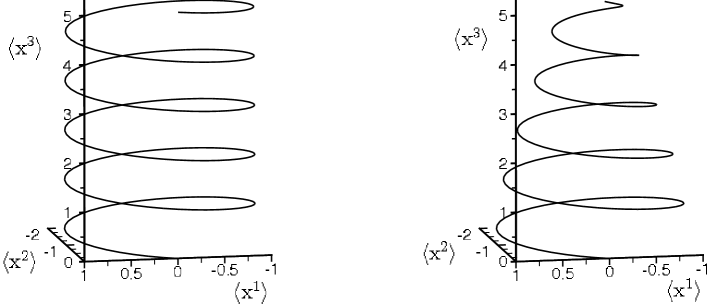
Figure 8: Typical trajectories traced by the expectation value of the position operator for a coherent state in a magnetic field with magnetic field parameter $\Lambda=0.001$, $\langle\Pi\rangle=2,\langle{\rm p}_{3}\rangle=1.6$, $\lambda_{3}=10^{-3},\lambda_{\perp}\simeq\sqrt{\Lambda}$ (left) and $\lambda_{3}=\lambda_{\perp}=0.25$ (right). $\langle{\rm x}^{1}\rangle$ and $\langle{\rm x}^{2}\rangle$ are given in unit of classical radius ($R_{\rm cl.}=\langle{\rm p}_{1}\rangle/\Lambda$), and $\langle{\rm x}^{3}\rangle$ is given in unit of ${\dot{x}}_{3}\tau_{\rm cl.}$, where ${\dot{x}}_{3}$ is the classical velocity in the parallel direction and $\tau_{\rm cl.}:=2\pi/\omega_{B}$ is the classical period of precession.

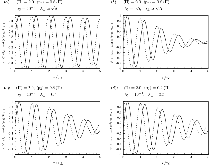
Figure 9: Plots of $\langle{\rm x}^{1}(\tau)\rangle$ (solid curve) and $\langle{\rm x}^{2}(\tau)\rangle+1$ (dashed curve) for various widths $\lambda_{\perp}$ and $\lambda_{3}$ with $\Lambda=0.01$, and $\langle\Pi\rangle=2.0$. $\langle{\rm x}^{1}(\tau)\rangle$ and $\langle{\rm x}^{2}(\tau)\rangle$ are scaled with the classical radius $R_{\rm cl.}$ and oscillate, with a decreasing amplitude, respectively like damped sine and cosine functions of the scaled time $\tau/\tau_{\rm cl.}$. $\tau_{\rm cl.}$ is classical period of precession. $\lambda_{\perp}\simeq\sqrt{\Lambda}$ means $|\lambda_{\perp}-\sqrt{\Lambda}|\leq 10^{-4}$. For $\lambda_{\perp}\rightarrow\sqrt{\Lambda}$ and small value of $\lambda_{3}$ the curves approach to the corresponding classical curves. The effect of $\lambda_{3}$ dominates that of $\lambda_{\perp}$. Also changing the initial transverse momentum does not affect the behavior of $\langle{\rm x}^{1}(\tau)\rangle$ and $\langle{\rm x}^{2}(\tau)\rangle$, though their magnitude clearly depends on the initial transverse momentum.

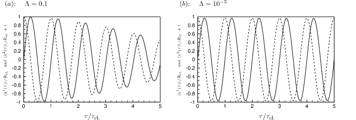
Figure 10: Plots of $\langle{\rm x}^{1}(\tau)\rangle$ (solid curve) and $\langle{\rm x}^{2}(\tau)\rangle+1$ (dashed curve) for two values of the magnetic field parameter $\Lambda=0.1,0.001$ with the same initial momentum $\langle\Pi\rangle=3,\langle{\rm p}_{3}\rangle=2.4$, and widths $\lambda_{3}=10^{-3},\lambda_{\perp}\simeq\sqrt{\Lambda}$. For $\lambda_{\perp}\rightarrow\sqrt{\Lambda}$ and small value of $\lambda_{3}$ the curves traced by the expectation value of the position operator approach the classical curves.

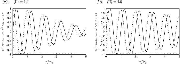
Figure 11: Plots of $\langle{\rm x}^{1}(\tau)\rangle$ (solid curve) and $\langle{\rm x}^{2}(\tau)\rangle+1$ (dashed curve) for $\Lambda=0.01$, $\langle\Pi\rangle=1$ and $4$, $\lambda_{3}=\lambda_{\perp}=0.25$ and $\langle{\rm p}_{3}\rangle=0.8\langle\Pi\rangle$. $\langle{\rm x}^{1}(\tau)\rangle$ and $\langle{\rm x}^{2}(\tau)\rangle$ are scaled with the classical radius and time is scaled with the classical period of precession. The higher the initial momentum becomes the closer the curves get to the corresponding classical curves.

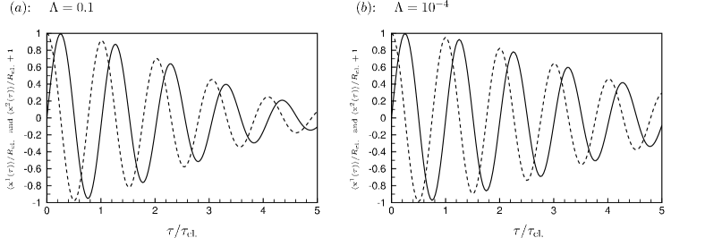
Figure 12: Plots of $\langle{\rm x}^{1}(\tau)\rangle$ (solid curve) and $\langle{\rm x}^{2}(\tau)\rangle+1$ (dashed curve) for $\Lambda=0.1$ and $10^{-4}$, $\langle\Pi\rangle=2,\langle{\rm p}_{3}\rangle=1.6$, and $\lambda_{3}=\lambda_{\perp}=0.25$. $\langle{\rm x}^{1}(\tau)\rangle$ and $\langle{\rm x}^{2}(\tau)\rangle$ are scaled with the classical radius and time is scaled with the classical period of precession. As the magnetic field decreases the curves approach the corresponding classical curves.

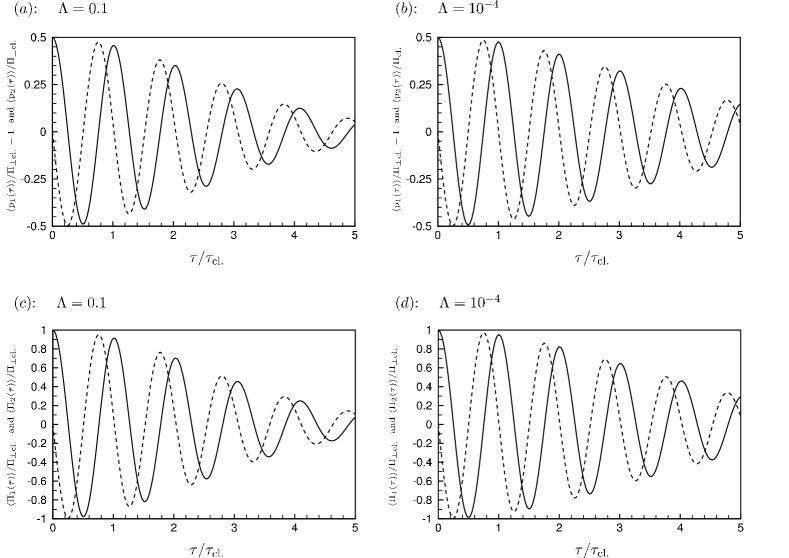
Figure 13: ($a$) and ($b$) are plots of $\langle{\rm p}_{1}(\tau)\rangle-1$ (solid curve), $\langle{\rm p}_{2}(\tau)\rangle$ (dashed curve), and ($c$) and ($d$) are plots of the transverse kinetic momentums $\langle\Pi_{1}(\tau)\rangle$ (solid curve) and $\langle\Pi_{2}(\tau)\rangle$ (dashed curve), for $\Lambda=0.1$ and $10^{-4}$, $\langle\Pi\rangle=2,\langle{\rm p}_{3}\rangle=1.6$, and $\lambda_{3}=\lambda_{\perp}=0.25$. The expectation value of the momentum operators are scaled with the corresponding classical transverse kinetic momentum $\Pi_{\perp}=\langle{\rm p}_{1}\rangle$ and the time is scaled with the classical period of precession. The behavior of $\langle{\rm p}_{1}(\tau)\rangle-1$ and $\langle\Pi_{1}(\tau)\rangle$ (resp. $\langle{\rm p}_{2}(\tau)\rangle$, and $\langle\Pi_{2}(\tau)\rangle$) reminisce the damped cosine (resp. sine) function. According to Eq. (99) the behavior of $\langle{\rm p}_{i}\rangle$ (and consequently $\langle\Pi_{i}\rangle$) is similar to that of $\langle{\rm x}_{i}\rangle$. Therefore, the higher the initial momentum (and the smaller the magnetic field) is the closer the curves traced by the expectation value of momentum operators are to the corresponding classical curves. Also for $\lambda_{\perp}\rightarrow\sqrt{\Lambda}$ and small value of $\lambda_{3}$ the curves approach to the classical ones.

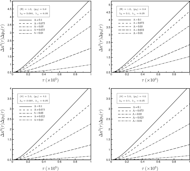
Figure 14: Plots of $(\Delta{\rm x}^{3})(\Delta{\rm p}_{3})$ as a function of time for different initial momentum expectation values, magnetic field parameter $\Lambda$, and the widths $\lambda_{3}$ and $\lambda_{\perp}$. $(\Delta{\rm x}^{3}(\tau))(\Delta{\rm p}_{3}(\tau))$ is an increasing function of the magnetic field. The presence of the magnetic field enhances the spreading of the wave packet. Also faster moving wave packets have a slower spreading rate.

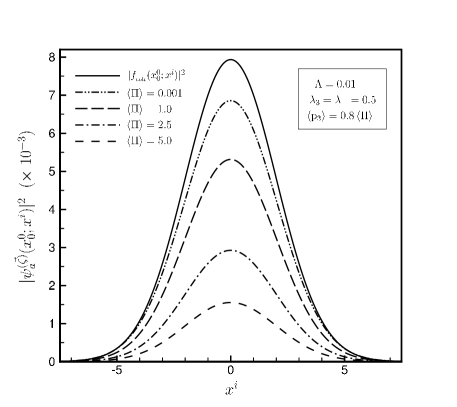
Figure 15: Plots of $|\psi_{a}^{(\vec{\zeta})}(x^{0}_{0};x^{i})|^{2}$ as a function of $x^{i}$ for $\Lambda=0.01$, where $|\psi_{a}^{(\vec{\zeta})}(x^{0}_{0};x^{i})|^{2}$ means $|\psi_{a}^{(\vec{\zeta})}(x^{0}_{0};\vec{x})|^{2}$ with $x^{j}=0$ if $j\neq i$. We has set $\kappa(1+\epsilon a)=1$. Since we consider the same widths along all three dimensions, (graphs of) $|\psi_{a}^{(\vec{\zeta})}(x^{0}_{0};x^{i})|^{2}$ are identical for all $i=1,2,3$. $|f_{{}_{\rm coh}}(x^{0}_{0};x^{i})|^{2}$, which is shown by the solid line, gives the nonrelativistic probability density. For smaller values of the momentum expectation value, i.e., in the nonrelativistic limit, $|\psi_{a}^{(\vec{\zeta})}(x^{0}_{0};x^{i})|^{2}$ tends to $|f_{{}_{\rm coh}}(x^{0}_{0};x^{i})|^{2}$.

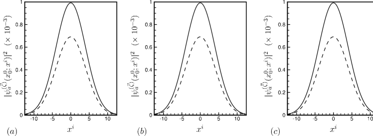
Figure 16: Plots of $|\psi_{a}^{(\vec{\zeta})}(x^{0}_{0};x^{i})|^{2}$ (dashed curve) with $\langle\Pi\rangle=1$ and $\lambda_{\perp}=\lambda_{3}=0.25$, for three values of the magnetic field parameter: $\Lambda=0.1$ ($a$), $\Lambda=10^{-3}$ ($b$) and $\Lambda=10^{-6}$ ($c$). The solid curve shows the nonrelativistic counterpart $|f_{{}_{\rm coh}}(x^{0}_{0};x^{i})|^{2}$. $|\psi_{a}^{(\vec{\zeta})}(x^{0}_{0};x^{i})|^{2}$ does not depend on the magnetic field parameter.

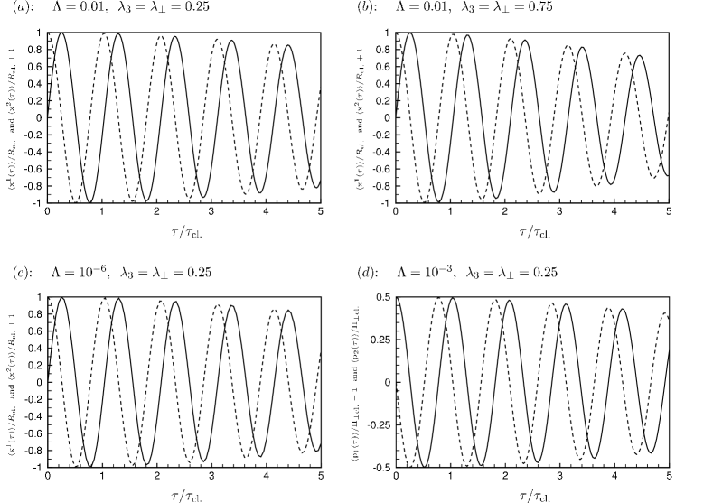
Figure 17: ($a$) – ($c$) are plots of $\langle{\rm x}^{1}(\tau)\rangle$ (solid curve) and $\langle{\rm x}^{2}(\tau)\rangle+1$ (dashed curve); ($d$) is the plots of $\langle{\rm p}_{1}(\tau)\rangle-1$ (solid curve) and $\langle{\rm p}_{2}(\tau)\rangle$ (dashed curve), for $\langle\Pi\rangle=10^{-3}$, different values of the magnetic field parameter $\Lambda$, and widths $\lambda_{3},\lambda_{\perp}$. The expectation value of position and momentum operators are scaled respectively with the classical radius and classical transverse kinetic momentum. Time is scaled with the classical period of precession. In the nonrelativistic limit ($c\rightarrow\infty$), the curves do not depend on either of the widths $\lambda_{\perp}$ and $\lambda_{3}$ or the magnetic field parameter $\Lambda$. They tend to the corresponding nonrelativistic curves obtained from Eqs. (107) and (108) which agree with the predictions of the classical theory.

Employing the “Gauss-Hermite routine of integration” [42], we have written and used a computer code in C++ to numerically perform the integrals and sums appearing in the above and following expressions for various expectation values. We present a summary of the results in Figs. 8 – 17 which we briefly elude to below.

Fig. 8 shows two typical trajectories traced by the expectation value of the position operator for the magnetic field parameter $\Lambda=0.001$, momentum expectation value $\langle\Pi\rangle=2,\langle{\rm p}_{3}\rangle=1.6$, and two cases of the initial widths of coherent state: $\lambda_{3}=10^{-3},\lambda_{\perp}\simeq\sqrt{\Lambda}$ and $\lambda_{3}=\lambda_{\perp}=0.25$. As indicated in this figure, for the first values of $\lambda_{3}$ and $\lambda_{\perp}$ the helix is very close to the classical result.

Figs. 9 – 12 show $\langle{\rm x}^{1}(\tau)\rangle$ and $\langle{\rm x}^{2}(\tau)\rangle+1$ as a function of time for five classical periods of precession. $\langle{\rm x}^{1}(\tau)\rangle$ and $\langle{\rm x}^{2}(\tau)\rangle+1$ oscillate respectively like damped sine and cosine functions. For $\lambda_{\perp}\rightarrow\sqrt{\Lambda}$ and smaller values of $\lambda_{3}$ the curves are closer to the corresponding classical curves. The effects of the width $\lambda_{3}$ is greater than the effect of $\lambda_{\perp}$. Also, changing the initial transverse momentum does not affect the behavior of $\langle{\rm x}^{1}(\tau)\rangle$ and $\langle{\rm x}^{2}(\tau)\rangle$, though their magnitude clearly depends on the initial transverse momentum. The higher the initial momentum and the smaller the magnetic field become the closer the curves of $\langle{\rm x}^{1}(\tau)\rangle$ and $\langle{\rm x}^{2}(\tau)\rangle+1$ get to the corresponding classical curves.

Fig. 13 shows $\langle{\rm p}_{1}(\tau)\rangle-1$, $\langle{\rm p}_{2}(\tau)\rangle$ and expectation value of transverse kinetic momenta $\langle\Pi_{1}(\tau)\rangle$ and $\langle\Pi_{2}(\tau)\rangle$ as functions of time for five classical periods of precession. $\langle{\rm p}_{1}(\tau)\rangle-1$ and $\langle\Pi_{1}(\tau)\rangle$ (respectively $\langle\Pi_{2}(\tau)\rangle$ and $\langle{\rm p}_{2}(\tau)\rangle$) oscillate like a damped cosine (resp. sine) function. As $\lambda_{\perp}\rightarrow\sqrt{\Lambda}$ and $\lambda_{3}\to 0$, the curves tend to their corresponding classical curves. Since the behavior of the momentum expectation value is similar to the position expectation value, we can conclude that as we increase the initial momentum and decrease the magnetic field the graphs of the components of the momentum expectation value tend to those of the classical momenta.

As indicated in these figures, the trajectories traced by the expectation value of the position and momentum operators do not coincide with the classical trajectories. The position expectation values trace a helix with a constant gyration center and a decreasing radius. Moreover the period of precession is smaller than the classical period. Note that because $\sqrt{(\langle{\rm x}^{1}\rangle-\langle{\rm x}^{1}_{\rm g.c.}\rangle)^{2}+(\langle{\rm x}^{2}\rangle-\langle{\rm x}^{2}_{\rm g.c.}\rangle)^{2}}$ is not the gyration radius, a decrease in this quantity as depicted in the graphs of Figs. 9 – 12 does not mean that the expectation value of the radius operator decreases. Indeed, if we identify the operators of the gyration center with

$${\rm x}^{1}_{\rm g.c.}:=\frac{{\rm x}^{1}}{2}+\frac{{\rm p}_{2}}{eB},~{}~{}~{}~{}~{}~{}~{}~{}~{}~{}~{}{\rm x}^{2}_{\rm g.c.}:=\frac{{\rm x}^{2}}{2}-\frac{{\rm p}_{1}}{eB},$$ (100)

which we have obtained by quantization of their classical counterparts, and use (95) – (99), we can easily see that the expectation value of these operators in the coherent state vector $|\vec{\zeta}\rangle$ are constant. This means that the gyration center is a constant point. Similarly we obtain the energy, radius, and angular momentum operators by quantization the corresponding classical quantities (72), (81) and (82). The expectation value of these operators in the coherent state vector $|\vec{\zeta}\rangle$ are also time-independent. They are given by

$$\langle E\rangle\! \!\!\!\!=\!\!\!\! \!{\cal E}\left\{\,\sum_{n=0}^{\infty}\sum_{\ell=-\infty}^{\infty}\frac{n!}{(n+|\ell|)!}\,\,s^{2n+|\ell|}u^{|\ell|}\!\left(L_{n}^{\!|\ell|}(u)\right)^{2}\right.$$ (101)

$$\vspace{2cm}\left.~{}~{}~{}~{}~{}~{}~{}~{}~{}~{}~{}~{}\times\int_{-\infty}^{+\infty}\!\!\!\!\!\!dk_{3}\,e^{-\frac{2}{\lambda_{3}^{2}}(k_{3}-\langle{\rm p}_{3}\rangle)^{2}}\!\!\sqrt{\Lambda(2n+1-\ell+|\ell|)+1+k_{3}^{2}}\,\right\},$$

$$\langle L_{3}\rangle\! \!\!\!\!=\!\!\!\! \!\frac{4\Lambda\lambda_{\perp}^{2}\,e^{-\frac{2\langle{\rm p}_{1}\rangle^{2}}{(\Lambda+\lambda_{\perp}^{2})}}}{(\Lambda+\lambda_{\perp}^{2})^{2}}\left\{\,\sum_{n=0}^{\infty}\sum_{\ell=-\infty}^{\infty}\!\!\ell\,\,\frac{n!}{(n+|\ell|)!}\,\,s^{2n+|\ell|}u^{|\ell|}\!\left(L_{n}^{\!|\ell|}(u)\right)^{2}\right\}=0,$$ (102)

$$\langle R\rangle\! \!\!\!\!=\!\!\!\! \!\frac{4\lambda_{\perp}^{2}\sqrt{\Lambda}\,e^{-\frac{2\langle{\rm p}_{1}\rangle^{2}}{(\Lambda+\lambda_{\perp}^{2})}}}{(\Lambda+\lambda_{\perp}^{2})^{2}}\left\{\,\sum_{n=0}^{\infty}\sum_{\ell=-\infty}^{\infty}\frac{n!}{(n+|\ell|)!}\,\,s^{2n+|\ell|}u^{|\ell|}\!\left(L_{n}^{\!|\ell|}(u)\right)^{2}\!\sqrt{2n+1-\ell+|\ell|}\right\},$$ (103)

$$\langle R^{2}\rangle\! \!\!\!\!=\!\!\!\! \!\frac{4\lambda_{\perp}^{2}\,e^{-\frac{2\langle{\rm p}_{1}\rangle^{2}}{(\Lambda+\lambda_{\perp}^{2})}}}{(\Lambda+\lambda_{\perp}^{2})^{2}}\left\{\,\sum_{n=0}^{\infty}\sum_{\ell=-\infty}^{\infty}\frac{n!}{(n+|\ell|)!}\,\,s^{2n+|\ell|}u^{|\ell|}\!\left(L_{n}^{\!|\ell|}(u)\right)^{2}\left(2n+1-\ell+|\ell|\right)\right\}$$ (104)

$$\!\!\!\!=\!\!\!\! \!\frac{\langle{\rm p}_{1}^{2}\rangle}{\Lambda^{2}}+\frac{(\Lambda^{2}+\lambda_{\perp}^{4})}{2\Lambda^{2}\lambda_{\perp}^{2}}=\langle R_{\rm g.c.}^{2}\rangle\,,$$

where we have performed the summations appearing in (104) by means of some useful identities listed in [40, 41], and in the last equality we have made use of (82) and (102). Note that $\langle R\rangle$, $\langle R^{2}\rangle$ and $\langle L_{3}\rangle$ do not depend on the width $\lambda_{3}$.

Tables 3 and 3 show some typical values of the expectation values of energy, $x^{3}$-component of the velocity, radius, square of radius, and dispersion in radius. The deviation from the classical values which is generally small diminishes for larger values of the initial momentum and the smaller values of the magnetic field.

​​$\langle\Pi\rangle,~{}\langle{\rm p}_{1}\rangle,~{}\lambda_{\perp}$ and $\lambda_{3}$​​		$\langle E\rangle/E_{\rm cl.}$	$\langle\dot{\rm x}^{3}\rangle/\dot{x}^{3}_{\rm cl.}$	$\langle R\rangle/R_{\rm cl.}$	$\langle R^{2}\rangle/R_{\rm cl.}^{2}$	$\Delta R/R_{\rm cl.}$
	$\lambda_{3}=10^{-3},~{}\lambda_{\perp}\simeq\sqrt{\Lambda}$	$1.00086$	$0.99943$	$1.00174$	$1.00694$	$0.05887$
$\langle\Pi\rangle=2$	$\lambda_{3}=0.5,~{}\lambda_{\perp}\simeq\sqrt{\Lambda}$	$1.00394$	$0.99022$	$1.00174$	$1.00694$	$0.05887$
$\langle{\rm p}_{1}\rangle=1.2$	$\lambda_{3}=10^{-3},~{}\lambda_{\perp}=0.5$	$1.01067$	$0.99286$	$1.02199$	$1.08694$	$0.20611$
	$\lambda_{3}=\lambda_{\perp}=0.5$	$1.01375$	$0.98383$	$1.02199$	$1.08694$	$0.20611$
	$\lambda_{3}=10^{-3},~{}\lambda_{\perp}\simeq\sqrt{\Lambda}$	$1.00074$	$0.99976$	$1.00097$	$1.00391$	$0.04417$
$\langle\Pi\rangle=2$	$\lambda_{3}=0.5,~{}\lambda_{\perp}\simeq\sqrt{\Lambda}$	$1.00521$	$0.98663$	$1.00097$	$1.00391$	$0.04417$
$\langle{\rm p}_{1}\rangle=1.6$	$\lambda_{3}=10^{-3},~{}\lambda_{\perp}=0.5$	$1.00932$	$0.99691$	$1.01230$	$1.04891$	$0.15539$
	$\lambda_{3}=\lambda_{\perp}=0.5$	$1.01375$	$0.98383$	$1.01230$	$1.04891$	$0.15539$
	$\lambda_{3}=\lambda_{\perp}=0.25$	$1.00063$	$0.99936$	$1.00089$	$1.00356$	$0.04218$
$\langle\Pi\rangle=5$	$\lambda_{3}=\lambda_{\perp}=0.5$	$1.00245$	$0.99745$	$1.00348$	$1.01391$	$0.08325$
$\langle{\rm p}_{1}\rangle=3$	$\lambda_{3}=0.25,~{}\lambda_{\perp}=0.5$	$1.00211$	$0.99849$	$1.00348$	$1.01391$	$0.08325$
	$\lambda_{3}=0.5,~{}\lambda_{\perp}=0.25$	$1.00097$	$0.99831$	$1.00089$	$1.00356$	$0.04218$

Table 2: Expectation values of energy, $x^{3}$-component of the velocity, radius, square of radius, and dispersion in radius are given for magnetic field parameter $\Lambda=0.01$ and various initial momenta and widths of the coherent state. The coherent states with smaller width and larger momentum display more pronounced classical behavior.

$\lambda_{\perp}$ and $\lambda_{3}$	$\Lambda$	$\langle E\rangle/E_{\rm cl.}$	$\langle\dot{\rm x}^{3}\rangle/\dot{x}^{3}_{\rm cl.}$	$\langle R\rangle/R_{\rm cl.}$	$\langle R^{2}\rangle/R_{\rm cl.}^{2}$	$\Delta R/R_{\rm cl.}$
$\lambda_{\perp}=0.25$	$\Lambda=0.1$	$1.01029$	$0.99133$	$1.01952$	$1.07725$	$0.19453$
$\lambda_{3}=0.25$	$\Lambda=10^{-4}$	$1.00344$	$0.99594$	$1.00544$	$1.02171$	$0.10385$
$\lambda_{\perp}=0.5$	$\Lambda=0.1$	$1.01547$	$0.98264$	$1.02553$	$1.10069$	$0.22128$
$\lambda_{3}=0.5$	$\Lambda=10^{-4}$	$1.01372$	$0.98385$	$1.02195$	$1.08681$	$0.20595$

Table 3: Expectation values of energy, $x^{3}$-component of the velocity, radius, square of radius, and dispersion in radius are given for magnetic field parameters $\Lambda=0.1,~{}10^{-4}$, initial momenta $\langle\Pi\rangle=2,~{}\langle{\rm p}_{3}\rangle=1.2$, and various widths $\lambda_{\perp}$ and $\lambda_{3}$. For smaller values of the magnetic field the results are closer to the corresponding classical quantities.

In the limit $B\rightarrow 0$ (equivalently $\Lambda\rightarrow 0$), Eqs. (95) – (98) and (101) reduce to the corresponding equations for a free KG field. For the case that the expectation value of the initial transverse momentum vanishes, i.e., $\langle{\rm p}_{i}\rangle=0$ for $i=1,2$, we find

$$\langle{\rm x}^{3}(\tau)\rangle \!\!\!\!=\!\!\!\! \frac{\tau}{\lambda_{3}}\sqrt{\frac{2}{\pi}}\int_{-\infty}^{+\infty}dk_{3}\,\frac{k_{3}\,e^{-\frac{2}{\lambda_{3}^{2}}(k_{3}-\langle{\rm p}_{3}\rangle)^{2}}}{\sqrt{1+k_{3}^{2}}},~{}~{}~{}~{}~{}~{}~{}\langle{\rm x}^{1}(\tau)\rangle=\langle{\rm x}^{2}(\tau)\rangle=0,$$

$$\langle E\rangle \!\!\!\!=\!\!\!\! \frac{1}{\lambda_{3}}\sqrt{\frac{2}{\pi}}\int_{-\infty}^{+\infty}dk_{3}\,\sqrt{1+k_{3}^{2}}\,e^{-\frac{2}{\lambda_{3}^{2}}(k_{3}-\langle{\rm p}_{3}\rangle)^{2}}.$$

Hence we have a free motion along $x^{3}$-direction.

Next, we determine the uncertainty relationship for ${\rm x}^{3}$ and ${\rm p}_{3}$ at an arbitrary time $\tau\in\mathbb{R}$. This yields

$$(\Delta{\rm x}^{3}(\tau))(\Delta{\rm p}_{3}(\tau))=\frac{1}{2}\sqrt{1+\lambda_{3}^{2}(\Delta\dot{\rm x}^{3})^{2}\,\tau^{2}},$$ (105)

where $(\Delta\dot{\rm x}^{3})^{2}:=\langle(\dot{\rm x}^{3})^{2}\rangle-\langle\dot{\rm x}^{3}\rangle^{2}$, $\langle\dot{\rm x}^{3}\rangle$ is given by (98), and

$$\langle(\dot{\rm x}^{3})^{2}\rangle \!\!\!\!=\!\!\!\! {\cal E}\left\{\,\sum_{n=0}^{\infty}\sum_{\ell=-\infty}^{\infty}\frac{n!}{(n+|\ell|)!}\,\,s^{2n+|\ell|}u^{|\ell|}\!\left(L_{n}^{\!|\ell|}(u)\right)^{2}\!\!\!\int_{-\infty}^{+\infty}\!\!\!\frac{k_{3}^{2}\,e^{-\frac{2}{\lambda_{3}^{2}}(k_{3}-\langle{\rm p}_{3}\rangle)^{2}}\,dk_{3}}{\Lambda(2n+1-\ell+|\ell|)+1+k_{3}^{2}}\right\}.$$

It is not difficult to check that in the limit $B\rightarrow 0$ (equivalently $\Lambda\rightarrow 0$) Eq. (105) reproduces the uncertainty relationship (58) for the free field.

Fig. 14 shows a plot of the right-hand side of (105) for different values of the initial momentum and the magnetic field. For the range of values of $\Lambda$ that are used in the graphs, $(\Delta{\rm x}^{3}(\tau))(\Delta{\rm p}_{3}(\tau))$ is an increasing function of the magnetic field. This also implies, in view of (105), that the presence of the magnetic field enhances the spreading of the wave packet. Moreover, similarly to the case of a free KG field, faster moving wave packets have a lower spreading rate.

Finally, using Eqs. (32), (83), (87), (92), (93), and inserting (94) in (87), we derive the functional form of a coherent KG field:

$$\psi_{a}^{(\vec{\zeta})}(x):=\psi_{a}^{(+,\vec{\zeta}_{+})}(x)\! \!\!\!\!=\!\!\!\! \!\frac{\sqrt{\Lambda{\cal E}}\,e^{-v/2}}{2\pi\sqrt{\kappa(1+a)}}\left\{\,\sum_{n=0}^{\infty}\sum_{\ell=-\infty}^{\infty}\!\!\!\left(\frac{n!}{(n+|\ell|)!}\right)\!e^{i\ell\varphi}(-s)^{n+|\ell|/2}(uv)^{|\ell|/2}L_{n}^{\!|\ell|}(v)L_{n}^{\!|\ell|}(u)\right.$$ (106)

$$\vspace{2cm}\left.\times\int_{-\infty}^{+\infty}\!\!\!\!\!\!\!dk_{3}\,e^{-\frac{1}{\lambda_{3}^{2}}(k_{3}-\langle{\rm p}_{3}\rangle)^{2}}e^{ik_{3}x^{3}}\frac{e^{-i(\tau-\tau_{0})\sqrt{\Lambda(2n+1-\ell+|\ell|)+1+k_{3}^{2}}}}{\left[\Lambda(2n+1-\ell+|\ell|)+1+k_{3}^{2}\right]^{1/4}}\right\},$$

where $v\!:=\!\Lambda\rho^{2}/2$. In the nonrelativistic limit ($c\rightarrow\infty$), $\psi_{a}^{(\vec{\zeta})}(x)$ tends to the nonrelativistic coherent wave function (87). This is consistent with Fig. 15 which gives the plots of $|f_{{}_{\rm coh}}(x^{0}_{0},\vec{x})|^{2}$ and $|\psi_{a}^{(\vec{\zeta})}(x^{0}_{0},\vec{x})|^{2}$ for various values of the momentum expectation value $\langle p\rangle_{\epsilon}=k\beta_{\epsilon}$ and the dimensionless widths $\lambda_{\perp},\lambda_{3}$. As seen from this figure, $|\psi_{a}^{(\vec{\zeta})}(x^{0}_{0},\vec{x})|^{2}$ depends on the expectation value of the initial momentum. In particular for smaller values of the initial momentum it tends to the nonrelativistic probability density $|f_{{}_{\rm coh}}(x^{0}_{0},\vec{x})|^{2}$.

Fig. 16 shows the plots of $|\psi_{a}^{(\vec{\zeta})}(x^{0}_{0},\vec{x})|^{2}$ for three different values of the magnetic field parameter $\Lambda$. A surprising behavior depicted in these plots, which is not evident from (106), is that $|\psi_{a}^{(\vec{\zeta})}(x^{0}_{0},\vec{x})|^{2}$ does not depend on the magnetic field. This observation suggests identifying the coherent states $|\vec{\zeta}\rangle$ of Eq. (86) as the appropriate nonrelativistic coherent states of a charged particle in a homogeneous magnetic field. To the best of our knowledge this identification has not been previously considered in the literatures [39, 13, 31].

Adopting (86) as the defining relation for nonrelativistic coherent states, we have computed the expectation values of position, momentum, energy, $x^{3}$-component of the velocity, radius, and angular momentum operators using the same method as for the relativistic coherent states. The result is

$$\langle{\rm x}^{1}(\tau)\rangle_{\rm nr} \!\!\!\!=\!\!\!\! \frac{\langle{\rm p}_{1}\rangle}{\Lambda}\,\sin{\Lambda\tau},~{}~{}~{}~{}~{}~{}\langle{\rm x}^{2}(\tau)\rangle_{\rm nr}=\frac{\langle{\rm p}_{1}\rangle}{\Lambda}\,\left(\cos{\Lambda\tau}-1\right),~{}~{}~{}~{}~{}~{}\langle{\rm x}^{3}(\tau)\rangle_{\rm nr}=\langle{\rm x}^{3}\rangle+\langle{\rm p}_{3}\rangle\,\tau,~{}~{}~{}~{}~{}~{}~{}~{}~{}~{}~{}$$ (107)

$$\langle{\rm p}_{1}(\tau)\rangle_{\rm nr} \!\!\!\!=\!\!\!\! \frac{\langle{\rm p}_{1}\rangle}{2}\,\left(\cos{\Lambda\tau}+1\right),~{}~{}~{}~{}~{}~{}~{}~{}\langle{\rm p}_{2}(\tau)\rangle_{\rm nr}=-\,\frac{\langle{\rm p}_{1}\rangle}{2}\,\sin{\Lambda\tau},~{}~{}~{}~{}~{}~{}~{}~{}\langle{\rm p}_{3}(\tau)\rangle_{\rm nr}=\langle{\rm p}_{3}\rangle.$$ (108)

$$\langle E\rangle_{\rm nr} \!\!\!\!=\!\!\!\! 1+\frac{\lambda_{3}^{2}}{8}+\frac{\langle{\rm p}_{3}\rangle^{2}}{2}+\frac{\Lambda^{2}\langle R^{2}\rangle_{\rm nr}}{2}=1+\frac{\lambda_{3}^{2}}{8}+\frac{\langle{\rm p}_{3}\rangle^{2}}{2}+\frac{\langle\Pi_{\perp}^{2}\rangle_{\rm nr}}{2},~{}~{}~{}~{}~{}~{}~{}\langle\dot{\rm x}^{3}(\tau)\rangle_{\rm nr}=\langle{\rm p}_{3}\rangle,$$ (109)

and $\langle R\rangle_{\rm nr}$, $\langle R^{2}\rangle_{\rm nr}$ and $\langle L_{3}\rangle_{\rm nr}$ have the same form as relativistic case. For $B=0$ (or $\Lambda=0$) Eq. (109) tends to the well-known result for the free particle (compare with (63)). These nonrelativistic expectation values do not depend on the widths $\lambda_{\perp}$ and $\lambda_{3}$ and coincide with the corresponding classical quantities. Using our numerical method, we have compared the relativistic and nonrelativistic results and checked that the former reproduces the latter, namely (107) – (109), in the nonrelativistic limit. Fig. 17 provides a graphical demonstration of this comparison.

Table 4 shows the energy and velocity expectation values obtained using the relativistic expression for a small value of the initial momentum. It also includes the nonrelativistic results obtained using (109). Relativistic and nonrelativistic calculations yield the same values for the expectation value of the radius $R$, square of radius $R^{2}$, and angular momentum $L_{3}$.

$\lambda_{\perp}$ and $\lambda_{3}$	$\Lambda$	$\langle E\rangle/E_{\rm cl.}$	$\langle E\rangle_{\rm nr}/E_{\rm cl.}$	$\langle\dot{\rm x}^{3}\rangle/\dot{x}^{3}_{\rm cl.}$
$\lambda_{\perp}=0.25$	$\Lambda=0.1$	$1.06127$	$1.06344$	$0.93013$
$\lambda_{3}=0.25$	$\Lambda=10^{-4}$	$1.02300$	$1.02344$	$0.96381$
$\lambda_{\perp}=0.5$	$\Lambda=0.1$	$1.09724$	$1.10375$	$0.87193$
$\lambda_{3}=0.5$	$\Lambda=10^{-4}$	$1.08764$	$1.09375$	$0.87959$

Table 4: Energy and velocity expectation values are given for the initial momentum expectation value $\langle\Pi\rangle=0.001$, magnetic field parameters $\Lambda=0.1,~{}10^{-4}$, and various widths $\lambda_{\perp}$ and $\lambda_{3}$. For all values of these parameters $\langle\dot{\rm x}^{3}\rangle_{\rm nr}/\dot{x}^{3}_{\rm cl.}=1$. Hence the data confirms that our relativistic calculations have the correct nonrelativistic limit.

6 Conclusion

In [12] we give a formulation of the quantum mechanics of first quantized scalar fields which is based on the construction of a genuine Hilbert space. This is determined by a one-parameter family of inner products $(\cdot,\cdot)_{a}$ where $a\in(-1,1)$. The Hilbert spaces ${\cal H}_{a}$ associated with different allowed values of $a$ are unitary-equivalent to $L^{2}(\mathbb{R}^{3})\oplus L^{2}(\mathbb{R}^{3})$. This allows for a straightforward construction of an appropriate pair of relativistic position and momentum operators and the corresponding relativistic coherent states.

In this paper we offer an explicit construction and a detailed investigation of the coherent states for both charged and neutral KG fields that are either free or interact with a constant homogeneous magnetic field. Our strategy is to construct coherent states in the two-component Foldy representation and pull them back using the appropriate unitary transformation to obtain coherent KG fields. In contrast to the earlier approaches to this problem, ours is free from the problems associated with the charge-superselection rule.

The general behavior of our coherent states are similar to that of a classical particle in both free and interacting cases. Moreover, in the nonrelativistic limit our results coincide with those of nonrelativistic quantum mechanics.

References

- [1] E. Schrödinger, Naturwissenschaften 14, 664 (1926); See also the interesting historical paper: F. Steiner, Physica B 151, 323 (1988).
- [2] R. J. Glauber, Phys. Rev. Lett. 10, 277 (1963); Phys. Rev. 130, 2529 (1963); Phys. Rev. 131, 2766 (1963).
- [3] E. C. G. Sudarshan, Phys. Rev. Lett. 10, 277 (1963).
- [4] J. R. Klauder, J. Math. Phys. 4, 1055 (1963); ibid 4, 1058 (1963).
- [5] J. R. Klauder, and B. S. Skagerstam, Coherent States, Applications in Physics and Mathematical physics (World Scientific Press, Singapour,1985).
- [6] A. M. Prelomov, Generalized Coherent States and their Applications (Springer, Berlin Heidelberg, 1986).
- [7] W. M. Zhang, et. al. Rev. Mod. Phys. 62, 867 (1990).
- [8] D. H. Feng, J. R. Klauder, and M. R. Strayer, Coherent States: Past, Present and Future (World Scientific, Singapour,1994).
-
[9]
B. Huttner, N. Imoto, N. Gisin, and
T. Mor, Phys. Rev. A 51, 1863 (1995);
T. C. Ralph, W. J. Munro, and G. J. Milburn, Proceedings of SPIE 4917, 1 (2002), quant-ph/0110115;
T. C. Ralph, A. Gilchrist, G. J. Milburn, W. J. Munro, and S. Glancy, Phys. Rev. A 68, 042319 (2003). - [10] A. M. Prelomov, Commun. Math. Phys. 26, 222 (1972).
- [11] R. Gilmore, Ann. Phys. (N.Y.) 74, 391 (1972).
- [12] A. Mostafazadeh, and F. Zamani, Quantum Mechanics of KG Fields I: Hilbert Space, Localized States, and Chiral Symmetry, quant-ph/0602151, to appear in Ann. Phys. (N.Y.).
- [13] I. A. Malkin and V. I. Man’ko, Sov. Phys. JETP 28, 527 (1969).
-
[14]
V. G. Bagrov, I. L. Buchbinder, and D. M. Gitman,
J. Phys. A: Math. Gen. 9, 1955 (1976); Izv. Vuzov. Fizica. 8, 134 (1975); Proceeding of the Group Theoretical
Methods in Physics,
Vol. 1, 232, 1979;
See Also: V. G. Bagrov, and D. M. Gitman, Exact Solution of Relativistic Wave Equations (Kluwer Academic Publishers, Bordrecht, 1990);
and V. G. Bagrov, M. C. Baldiotti, D. M. Gitman, and I. V. Shirokov, J. Math. Phys. 43, 2284 (2002). - [15] B. I. Lev, A. A. Semenov, C. V. Usenko, and J. R. Klauder, Phys. Rev. A 66, 02215 (2002).
- [16] M. Haghighat and A. Dadkhah, Phys. Lett. A 316, 271 (2003).
- [17] J. C. Botke, D. J. Scalapino, and R. L. Sugar, Phys. Rev. D 9, 813 (1974).
- [18] D. Bhaumik, K. Bhaumik, and B. Dutta-Roy, J. Phys. A: Math. Gen. 9, 1507 (1976).
- [19] B. S. Skagerstam, Phys. Rev. D 19, 2471 (1979); ibid 22, 534 (1980).
- [20] V. Aldaya and J. Guerrero, J. Math. Phys. 36, 3191 (1995).
- [21] J. Tang, Phys. Lett. A 229, 33 (1996).
- [22] T. R. Field and L. P. Hughston, J. Math. Phys. 40, 2568 (1999).
- [23] T. D. Newton and E. P. Wigner, Rev. Mod. Phys. 21, 400 (1949).
-
[24]
M. H. L. Pryce, Procc. Roy. Soc. London A 195, 62 (1948);
A. S. Wightman, Rev. Mod. phys. 34, 845 (1962);
T. F. Jordan and N. Mukunda, Phys. Rev. 132, 0842 (1963);
T. O. Philips, Phys. Rev. 136, B893 (1964);
H. Bacry, J. Math. Phys. 1, 109 (1964);
R. A. Berg, J. Math. Phys. 6, 109 (1965);
A. Sankaranarayanan and R. H. Good, Jr., Phys. Rev. 140, B509 (1965);
J. E. Johnson, Phys. Rev. 181, 1755 (1969);
R. F. O’Connell and E. P. Wigner, Phys. Lett. 67 A, 319 (1978);
T. F. Jordan, J. Math. Phys. 21, 2028 (1980). - [25] H. Feshbach and F. Villars, Rev. Mod. Phys. 30, 24 (1958).
- [26] A. Mostafazadeh, preprint: quant-ph/0307059, to appear in Int. J. Mod. Phys. A.
- [27] W. Greiner, Relativistic Quantum Mechanics (Springer, Berlin, 1994).
- [28] G. C. Wick A. S. Wightman and E. P. Wigner, Phys. Rev. 88, 101 (1952).
- [29] R. L. de Matos Filho, and W. Vogel, Phys. Rev. A 54, 4560 (1996).
- [30] A. Mostafazadeh, Ann. Phys. (N.Y.) 309, 1 (2004).
- [31] C. Cohen-Tannoudji, B. Diu, and F. Laloë, Quantum Mechanics, Vol. 1, (John Wiley and Sons, 1978).
- [32] E. Merzbacher, Quantum Mechanics, Second Edition, (John Wiley and Sons, 1970).
- [33] A. J. Bracken, and G. F. Melloy, J. Phys. A: Math. Gen. 32, 6127 (1999).
- [34] B. Thaller, Visual Quantum Mechanics (Springer-Verlag, 2000)
-
[35]
D. M. Gitman and I. V. Tyutin, Class. Quantum
Grav. 7, 2131 (1990);
S. P. Gavrilov and D. M. Gitman, Class. Quantum Grav. 17, L133 (2000) and Int. J. Mod. Phys. A 15, 4499 (2000). - [36] J. D. Jacskon, Classical Electrodynamics (John Wiley and Sons, 1975).
- [37] M. H. Johnson and B. A. Lippmamn, Phys. Rev. 76, No. 6, 828 (1949).
- [38] H. J. Briegel, et.al., Naturforsch. A: Phys. Sci. 46, 934 (1991).
- [39] K. Kowalski, and J. Rembieliński, J. Phys. A: Math. Gen. 38, 8247 (2005).
- [40] I. S. Gradshteyn, and I. M. Ryzhik, Table of Integrals, Series, and Products, 6th ed., (Academic Press, USA, 2000).
- [41] N. N. Lebedev, Special Functions and Their Applications, (Dover Publications, 1972).
- [42] W. H. Press, S. A. Teucolsky, W. T. Vetterling, and B. P. Flannery, Numerical Recipes, 2nd ed., (Cambridg University Press, U.K., 1992).