Universal and phase covariant superbroadcasting for mixed qubit states

Abstract

We describe a general framework to study covariant symmetric broadcasting maps for mixed qubit states. We explicitly derive the optimal $N\to M$ superbroadcasting maps, achieving optimal purification of the single-site output copy, in both the universal and the phase covariant cases. We also study the bipartite entanglement properties of the superbroadcast states.

I Introduction

“Information” is by its nature broadcastable. What happens when information is quantum and we need to distribute it among many users? Indeed, this may be useful in all situations where quantum information is required in sharable form, e. g. in distributed quantum computation discom , for quantum shared secrecy shacrip , and, generally, in quantum game-theoretical contexts gam . However, contrarily to the case of classical information, which can be distributed at will, broadcasting quantum information can be done only in a limited fashion. Indeed, for pure states ideal broadcasting is equivalent to the so-called “quantum cloning”, which is impossible due to the well-known “no-cloning” theorem Wootters82 ; Dieks82 ; Yuen (see also noteclon ; darianoyuen ; herbert ; peres ). The situation is more involved when the input states are mixed, since broadcasting can be achieved with an output joint state which is indistinguishable from the tensor product of local mixed states from the point of view of individual receivers. Therefore, the no cloning theorem cannot logically exclude the possibility of ideal broadcasting for sufficiently mixed states.

In Ref. Barnum96 it was proved that perfect broadcasting is impossible from a single input copy to two output copies for an input set of non mutually commuting density operators. This result was then considered (see Refs. Barnum96 and clifton ) as an evidence of the general impossibility of broadcasting mixed states drawn from a non-commuting set in a more general scenario, where $N\geqslant 1$ equally prepared input copies are broadcast to $M>N$ users. However, for sufficiently many input copies $N$ and sufficiently mixed input states the no-broadcasting theorem does not generally hold our , and for input mixed states drawn from a noncommuting set it is possible to generate $M>N$ output local mixed states which are identical to the input ones, by a joint correlated state. Actually, as proved in Ref. our , it is even possible to partially purify the local state in the broadcasting process, for sufficiently mixed input states. Such a process of simultaneous purification and broadcasting was named superbroadcasting. For qubits, the fully covariant superbroadcasting channel that maximizes the output purity (i. e. the length of the output Bloch vectors of local states) when applied to input pure states coincides with the optimal cloning map Werner98 .

The possibility of superbroadcasting does not increase the available information about the original input state, due to unavoidable detrimental correlations among the local broadcast copies, which do not allow to exploit their statistics (a similar phenomenon was already noticed in Ref. Keyl01 ). Essentially, superbroadcasting transfers noise from local states to correlations. From the point of view of single users, however, the protocol is a purification in all respects, and this opens new interesting perspectives in the ability of distributing quantum information in a noisy environment, and deserves to be analyzed in depth. For qubits, it has been shown that for universal superbroadcasting is possible with at least $N=4$ input copies our . Is this the absolute minimum number for superbroadcasting, or does it hold only for this particular set of input states? In this paper we will show that, indeed, for equatorial mixed states of qubits the minimum number is $N=3$. However, for smaller non-commuting sets of qubit states the possibility of superbroadcasting with only $N=2$ input copies is still an open problem (for larger dimension $d>2$ it is possible to superbroadcast also for $N=2$, see e.g. Ref. cvsb ).

We want to point put that clearly there are limitations to superbroadcasting. The input state must be indeed sufficiently mixed, since pure states cannot be broadcast by the no cloning theorem. However, states with a pretty high purity can sill be superbroadcast, e. g. for universally covariant superbroadcasting our from $N=4$ to $M=5$ it is possible to superbroadcast states with a Bloch vector length up to 0.787 (0.935 for the phase covariant case). One can achieve superbroadcasting with even higher input purity for increasing $N$, approaching unit input Bloch vector length in the limit of infinitely many input copies. There are also some limitations in the absolute number of output copies for which one can achieve superbroadcasting. E. g. in the universal case, for $N=4$ input copies one can superbroadcast up to $M=7$ output copies, for $N=5$ up to $M=22$, and for $N>5$ up to infinitely many. The output purity is clearly decreasing versus $M$. In this paper we will further analyze all limitations to superbroadcasting also for the case of equatorial input qubits.

Regarding the possibility of achieving superbroadcasting experimentally, the first route to explore is to use the same techniques as for purification Cirac99 , since the superbroadcasting map for $M>N$ generalizes the purification map using the same protocol altro . This transformation involves a measurement of the total angular momentum of the qubits, then an optimal Werner cloning Werner98 in the universal case (or an optimal phase covariant cloning purequbitqutrit in the phase covariant case). Another possibility is to use the methods of Ref. Buscemi03 in order to classify all possible unitary realizations, and then seek for experimentally achievable ones using current technology.

In this paper we present phase covariant superbroadcasting, and also give a complete derivation of the universal superbroadcasting map, presented in Ref. our . The two maps are derived in a unified theoretical framework. The paper is organized as follows. In Section II we introduce some preliminary notions regarding symmetric covariant maps. In Sects. III and IV we give a complete derivation of the optimal broadcasting maps in the universal case and in the phase covariant case respectively. In Sect. V we study the entanglement properties of the states of two copies at the output of the universal and the phase covariant broadcasting maps. Finally, in Sect. VI we summarize and comment the main results of this paper. At the end of the paper we report the details of the calculations needed to derive the results presented in three appendices.

II Symmetric qubits broadcasting

In this Section we introduce in a unified theoretical framework some preliminary concepts that will be employed to describe covariant symmetric qubit broadcasting maps. These concepts will be then specified to the universal and the phase covariant cases in the subsequent sections. A main tool we will extensively use in deriving the optimal maps is the formalism of the Choi-Jamiołkowski isomorphism choi-jam between completely positive (CP) maps $\mathcal{E}$ from states on the Hilbert space $\mathscr{H}$ to states on the Hilbert space $\mathscr{K}$, and positive bipartite operators $R$ on $\mathscr{K}\otimes\mathscr{H}$. Such an isomorphism can be specified as follows

$$R\doteq\mathcal{E\otimes I}(|\Omega\rangle\langle\Omega|)\longleftrightarrow\mathcal{E}(\rho)\doteq\operatorname{Tr}_{\mathscr{H}}[\openone\otimes\rho^{T}\ R],$$ (1)

where $\Omega$ is the non normalized maximally entangled state $\sum_{m}|\psi_{m}\rangle\otimes|\psi_{m}\rangle$ in $\mathscr{H}\otimes\mathscr{H}$, $\mathcal{I}$ gives the identity transformation and $X^{T}$ denotes the transposition of the operator $X$ on the same basis $|\psi_{m}\rangle$ used in the definition of $\Omega$.

In terms of $R$, the trace-preservation condition for the map $\mathcal{E}$ reads

$$\operatorname{Tr}_{\mathscr{K}}[R]=\openone_{\mathscr{H}}\,.$$ (2)

Suppose that the map $\mathcal{E}$ is covariant under the action of a group $\bf G$. In this case the covariance property is reflected to the form of the operator $R$ by the following correspondence

$$\mathcal{E}(U_{g}\rho U_{g}^{\dagger})\equiv V_{g}\mathcal{E}(\rho)V_{g}^{\dagger}\Longleftrightarrow[V_{g}\otimes U_{g}^{*},R]=0.$$ (3)

In the above expression $U_{g}$ and $V_{g}$ are the unitary representations of ${\bf G}\ni g$ on the input and output spaces respectively, while $X^{*}$ denotes complex conjugation on the fixed basis $|\psi_{m}\rangle$. In this framework it is also possible to study group-invariance properties of the map $\mathcal{E}$ in terms of the operator $R$. In this case we have the following equivalences

$$\mathcal{E}(U_{g}\rho U_{g}^{\dagger})\equiv\mathcal{E}(\rho)\Longleftrightarrow[\openone\otimes U_{g}^{*},R]=0,$$ (4)

and

$$\mathcal{E}(\rho)\equiv V_{g}\mathcal{E}(\rho)V_{g}^{\dagger}\Longleftrightarrow[V_{g}\otimes\openone,R]=0.$$ (5)

The above expressions refer to invariance properties on the input and output spaces respectively.

In the following we will consider maps $\mathcal{B}$ from states of $N$ qubits to states of $M$ qubits, namely CP maps from states on $\mathscr{H}=(\mathbb{C}^{2})^{\otimes N}$ to states on $\mathscr{K}=(\mathbb{C}^{2})^{\otimes M}$. We will consider in particular symmetric broadcasting maps, namely transformations where all receivers get the same reduced state. The figures of merit which are commonly used are invariant under permutations of the output copies, and this allows to assume that the output state of a broadcasting map is permutation invariant without loss of generality. Moreover, since the input consists in $N$ copies of the same state, there is no loss of generality in requiring that the map is also invariant under permutations of the input copies. These two properties, according to Eqs. (4, 5), can be recast as follows

$$[\Pi_{\sigma}^{M}\otimes\Pi_{\tau}^{N},R]=0,\qquad\forall\sigma,\tau,$$ (6)

where $\Pi_{\sigma}^{M}$ and $\Pi_{\tau}^{N}$ are representations of the output and input copies permutations, respectively. Notice that permutations representations are all real, hence $\Pi_{\sigma}^{*}=\Pi_{\sigma}$.

A useful tool to deal with unitary group representations $U_{g}$ of a group $\bf G$ on a Hilbert space $\mathscr{H}$ is the Wedderburn decomposition of $\mathscr{H}$

$$\mathscr{H}\simeq\bigoplus_{\mu}\mathscr{H}_{\mu}\otimes\mathbb{C}^{d_{\mu}}\,,$$ (7)

where the index $\mu$ labels the equivalence classes of irreducible representations which appear in the decomposition of $U_{g}$. The spaces $\mathscr{H}_{\mu}$ support the irreducible representations and $\mathbb{C}^{d_{\mu}}$ are the multiplicity spaces, with dimension $d_{\mu}$ equal to the degeneracy of the $\mu$-th irreducible representation. Correspondingly the representation $U_{g}$ decomposes as

$$U_{g}=\bigoplus_{\mu}U_{g}^{\mu}\otimes\openone_{d_{\mu}},$$ (8)

where $\openone_{d_{\mu}}$ is shorthand for $\openone_{{\mathbb{C}}^{d_{\mu}}}$. By Schur’s Lemma, every operator $X$ commuting with the representation $U_{g}$ in turn decomposes as

$$X=\bigoplus_{\mu}\openone_{\mathscr{H}_{\mu}}\otimes X_{d_{\mu}}.$$ (9)

In the case of permutation invariance, the so-called Schur-Weyl duality fulton holds, namely the spaces $\mathbb{C}^{d_{\mu}}$ for permutations of $M$ qubits coincide with the spaces $\mathscr{H}_{\mu}$ for the representation $U_{g}^{\otimes M}$ of $\mathbb{SU}(2)$, where $U_{g}$ is the defining representation. In other words, a permutation invariant operator $Y$ can act non trivially only on the spaces $\mathscr{H}_{\mu}$, namely it can be decomposed as

$$Y=\bigoplus_{\mu}Y_{\mu}\otimes\openone_{d_{\mu}}.$$ (10)

The Clebsch-Gordan series for the defining representation of $\mathbb{SU}(2)$ is well-known in the literature (see for example fulton ; edmonds ), and its Wedderburn decomposition is given by

$$\mathscr{H}\simeq\bigoplus_{j=j_{0}}^{M/2}\mathscr{H}_{j}\otimes\mathbb{C}^{d_{j}}\,,$$ (11)

where $\mathscr{H}_{j}=\mathbb{C}^{2j+1}$, $j_{0}$ equals 0 for $M$ even, 1/2 for $M$ odd, and

$$d_{j}=\frac{2j+1}{M/2+j+1}\binom{M}{M/2-j}.$$ (12)

In the case of the broadcasting maps the Hilbert space $\mathscr{K}\otimes\mathscr{H}$ on which the operator $R$ acts, supports the two permutation representations corresponding to the output and input qubits permutations. Therefore it can be decomposed as

$$\mathscr{K}\otimes\mathscr{H}\simeq\left(\bigoplus_{j=j_{0}}^{M/2}\mathscr{H}_{j}\otimes\mathbb{C}^{d_{j}}\right)\otimes\left(\bigoplus_{l=l_{0}}^{N/2}\mathscr{H}_{l}\otimes\mathbb{C}^{d_{l}}\right)\,.$$ (13)

By rearranging the factors in the above expression, we can recast the decomposition in a more suitable way, namely

$$\mathscr{K}\otimes\mathscr{H}\simeq\bigoplus_{j=j_{0}}^{M/2}\bigoplus_{l=l_{0}}^{N/2}\left(\mathscr{H}_{j}\otimes\mathscr{H}_{l}\right)\otimes\left(\mathbb{C}^{d_{j}}\otimes\mathbb{C}^{d_{l}}\right)\,.$$ (14)

The operator $R$, in order to satisfy the permutation invariance property (6), according to Eq. (10), can be written in the following form

$$R=\bigoplus_{j=j_{0}}^{M/2}\bigoplus_{l=l_{0}}^{N/2}R_{jl}\otimes\left(\openone_{d_{j}}\otimes\openone_{d_{l}}\right)\,,$$ (15)

where the operators $R_{jl}$ act on $\mathscr{H}_{j}\otimes\mathscr{H}_{l}$. Moreover, in order to fulfill the requirements of trace preservation and complete positivity, the operators $R_{jl}$ must satisfy the constraints

$$R_{jl}\geqslant 0\,,\quad\operatorname{Tr}_{j}[R_{jl}]=\frac{\openone_{2l+1}}{d_{j}},$$ (16)

where $\operatorname{Tr}_{j}$ denotes the partial trace performed over the space $\mathscr{H}_{j}$ in the $j$-th term of the decomposition in Eq. (14), and $\openone_{2l+1}$ is shorthand for $\openone_{\mathscr{H}_{l}}$. We have now all the tools to study symmetric qubits broadcasting devices. In this work we are interested in the case of covariant broadcasting maps, which in general have to fulfill also the following covariance condition under the representations $V_{g}^{\otimes N}$ and $V_{g}^{\otimes M}$ of a group $\bf G$ (see Eq. (3))

$$\left[V_{g}^{\otimes M}\otimes{V_{g}^{*}}^{\otimes N},R\right]=0.$$ (17)

The above condition gives a further constraint on the form of the operators $R_{jl}$ in Eq. (15). Actually, the group $V_{g}$ is in general just a subgroup of the defining representation $U_{g}$ of $\mathbb{SU}(2)$, and therefore the representation $V_{g}^{\otimes M}\otimes{V_{g}^{*}}^{\otimes N}$ acts non trivially only on the subspaces $\mathscr{H}_{j}\otimes\mathscr{H}_{l}$, which are the ones supporting the operators $R_{jl}$. In the next sections we will consider two interesting cases, namely $V_{g}\equiv U_{g}$ and $V_{g}\equiv V_{\phi}=e^{i\frac{\phi}{2}\sigma_{z}}$, corresponding to universal and phase covariant broadcasting respectively, and we will see how the form of the operators $R_{jl}$ depends on the particular choice of the considered covariance group.

In addition to the Wedderburn decomposition and the related Schur-Weyl duality reviewed above, another useful tool we will extensively use in the following is a convenient decomposition of an $N$-partite state of the form $\rho^{\otimes N}$, representing $N$ qubits all prepared in the same generic state $\rho$. In Appendix A we report the complete derivation of the following identity, which was originally presented in Cirac99 ,

$$\rho^{\otimes N}=(r_{+}r_{-})^{N/2}\bigoplus_{j=j_{0}}^{N/2}\sum_{m=-j}^{j}\left(\frac{r_{+}}{r_{-}}\right)^{m}|jm\rangle\langle jm|\otimes\openone_{d_{j}}.$$ (18)

For the sake of simplicity, in the above expression we considered density operators of the form $\rho=(\openone+r\sigma_{z})/2$, $r_{\pm}=(1\pm r)/2$, namely qubit states whose Bloch vector (of length $r$) is aligned along the $z$ axis, and consequently the states $|jm\rangle$ are eigenstates of the operator $J_{z}$ in the $j$ representation, namely $J_{z}^{(j)}=\sum_{m=-j}^{j}m|jm\rangle\langle jm|$. Notice actually that the total angular momentum component $J_{z}$ of $N$ qubits is clearly permutation invariant and therefore it can be written as

$$J_{z}=\bigoplus_{j=j_{0}}^{N/2}J_{z}^{(j)}\otimes\openone_{d_{j}}.$$ (19)

We want to point out that the decomposition (18) holds for any direction of the Bloch vector, provided that the eigenstates of $J_{z}$ in Eq. (18) are replaced by the eigenvectors of the angular momentum component along the direction of the Bloch vector in the single qubit state $\rho$.

We will prove in Appendix C that the single-site output copy $\rho^{\prime}$ of a covariant broadcasting map commutes with the input density operator $\rho$. In order to quantify the performance of the broadcasting map $\mathcal{B}$ and to judge the quality of the single-site output density operator $\rho^{\prime}=\operatorname{Tr}_{M-1}[\mathcal{B}(\rho^{\otimes N})]$ we will then evaluate the length $r^{\prime}$ of its Bloch vector, namely

$$\operatorname{Tr}[\sigma_{z}\rho^{\prime}]=r^{\prime}\,.$$ (20)

Notice, moreover, that the length of a Bloch vector $r$ is simply related to the purity $\operatorname{Tr}[\rho^{2}]$ of the density operator $\rho$ as $\operatorname{Tr}[\rho^{2}]=(1+r^{2})/2$. Therefore, maximizing the output Bloch vector length $r^{\prime}$ is equivalent to maximizing the output single-site purity. Notice also that so far we cannot exclude that the input and output Bloch vectors $r$ and $r^{\prime}$ are antiparallel, and this just implies that $r^{\prime}$ can range from $-1$ to $1$.

We will now show how to evaluate $r^{\prime}$ according to Eq. (20), which is the main quantity that we will consider in the next sections in the particular cases of universal and phase covariant broadcasting. The trace in Eq. (20) can be computed by considering that the global output state $\Sigma=\mathcal{B}(\rho^{\otimes N})$ of the $M$ copies is by construction invariant under permutations, hence

$$r^{\prime}=\operatorname{Tr}[\sigma_{z}\rho^{\prime}]=\operatorname{Tr}\left[\left(\sigma_{z}\otimes\openone^{\otimes M-1}\right)\Sigma\right]=\frac{1}{M!}\operatorname{Tr}\left[\sum_{\sigma}\Pi_{\sigma}\left(\sigma_{z}\otimes\openone^{\otimes M-1}\right)\Pi_{\sigma}\Sigma\right]\,.$$ (21)

The last term on the r.h.s. of Eq. (21) contains a sum over the $M!$ possible permutations of the $M$ output qubits. Notice that

$$\frac{1}{M!}\sum_{\sigma}\Pi_{\sigma}(\sigma_{z}\otimes\openone^{\otimes(M-1)})\Pi_{\sigma}=\frac{1}{M}\sum_{i=1}^{M}\sigma_{z}^{(i)}=\frac{2}{M}J_{z}\,,$$ (22)

where the operator $\sigma_{z}^{(i)}$ acts as $\sigma_{z}$ on the $i$-th qubit and identically on the remaining qubits. Now, by exploiting the permutation invariance of $\Sigma$, we can write

$$\Sigma=\bigoplus_{j=j_{0}}^{M/2}\Sigma_{j}\otimes\openone_{d_{j}}\,,$$ (23)

and clearly

$$r^{\prime}=\frac{2}{M}\sum_{j=j_{0}}^{M/2}d_{j}\operatorname{Tr}[J_{z}^{(j)}\Sigma_{j}]\,.$$ (24)

The explicit expression of $r^{\prime}$ in the universal case will be derived in Sect. III. In the phase covariant case, we will see that it is more convenient to take $\rho$ diagonal on the $\sigma_{x}$ eigenstates. The above formula in this case is just substituted by

$$r^{\prime}=\frac{2}{M}\sum_{j=j_{0}}^{M/2}d_{j}\operatorname{Tr}[J_{x}^{(j)}\Sigma_{j}]\,$$ (25)

and will be explicitly calculated in Sect. IV.

We want to stress that maximization of the figure of merit $r^{\prime}$ allows to optimize the fidelity criterion as well. In fact, for $r^{\prime}<r$ the two criteria coincide, whereas for $r^{\prime}\geqslant r$ one can always achieve unit fidelity by suitably mixing the output state with optimal $r^{\prime}$ and the maximally mixed one. On the other hand, direct maximization of fidelity is not analytically feasible, since fidelity is a concave function over the convex set of covariant maps, whence it is not maximized by extremal maps.

Finally, we want to mention that in the next sections we explicitly maximize the scaling factor for $N$ inputs and $M$ outputs $p^{N,M}(r)\equiv r^{\prime}/r$, which can be referred to as shrinking factor or stretching factor, depending whether it is smaller or greater than 1, respectively. It is obvious that this maximization is equivalent to maximizing $r^{\prime}$. Superbroadcasting corresponds to the cases where $p(r)>1$.

III universal case

In this Section we will give the explicit derivation of the optimal universal broadcasting maps. Starting from the general broadcasting map described in the previous section we have to impose in this case the additional constraint

$$[U_{g}^{\otimes M}\otimes{U_{g}^{*}}^{\otimes N},R]=0\,,$$ (26)

where $U_{g}$ is the defining representation of the group $\mathbb{SU}(2)$. For the defining representation $U_{g}$ the following property holds

$$U_{g}^{*}=\sigma_{y}U_{g}\sigma_{y}\,.$$ (27)

By exploiting such a property, the commutation relation (26) can be written more conveniently as follows

$$[U_{g}^{\otimes(M+N)},S]=0\,,$$ (28)

where $S=(\openone^{\otimes M}\otimes\sigma_{y}^{\otimes N})R(\openone^{\otimes M}\otimes\sigma_{y}^{\otimes N})=\left(\openone^{\otimes M}\otimes e^{i\pi J_{y}}\right)R\left(\openone^{\otimes M}\otimes e^{-i\pi J_{y}}\right)$. The complete positivity and trace-preservation constraints in terms of the operator $S$ are then equivalent to

$$S\geqslant 0\,,\quad\operatorname{Tr}_{\mathscr{K}}[S]=\openone_{\mathscr{H}}\,.$$ (29)

Upon defining $S_{jl}=\left(\openone_{2j+1}\otimes e^{i\pi J^{(l)}_{y}}\right)R_{jl}\left(\openone_{2j+1}\otimes e^{-i\pi J^{(l)}_{y}}\right)$, the constraints for complete positivity and trace preservation are now given by the following conditions on the operators $S_{jl}$

$$S_{jl}\geqslant 0\,,\quad\operatorname{Tr}_{j}[S_{jl}]=\frac{\openone_{2l+1}}{d_{j}}.$$ (30)

By exploiting the fact that the Clebsch-Gordan series for $\mathscr{H}_{j}\otimes\mathscr{H}_{l}$ is just $\bigoplus_{J=|j-l|}^{j+l}\mathscr{H}_{J}$, we can write

$$\mathscr{K}\otimes\mathscr{H}=\bigoplus_{j=j_{0}}^{M/2}\bigoplus_{l=l_{0}}^{N/2}\bigoplus_{J=|j-l|}^{j+l}\mathscr{H}^{j,l}_{J}\otimes\mathbb{C}^{d_{j}}\otimes\mathbb{C}^{d_{l}}\,.$$ (31)

Notice that this is not the Wedderburn decomposition, since not all the subspaces $\mathscr{H}^{j,l}_{J}\simeq\mathbb{C}^{2J+1}$ support inequivalent representations. However, the Wedderburn decomposition can be recovered by a suitable rearrangement that takes into account the repetitions of the same representation $J$. Using the decomposition (31) we can formulate the constraint (28) in terms of the operators $S_{jl}$ as follows

$$S_{jl}=\bigoplus_{J=|j-l|}^{j+l}s_{j,l}^{J}P_{j,l}^{J}\,,$$ (32)

where, by complete positivity, the coefficients $s_{j,l}^{J}$ are real and positive, and $P_{j,l}^{J}$ is the projection of the space $\mathscr{H}_{j}\otimes\mathscr{H}_{l}$ onto the $J$ representation, satisfying

$$\operatorname{Tr}_{j}\left[P^{J}_{j,l}\right]=\frac{2J+1}{2l+1}\openone_{2l+1},\qquad\operatorname{Tr}_{l}\left[P^{J}_{j,l}\right]=\frac{2J+1}{2j+1}\openone_{2j+1}.$$ (33)

The set of projectors $P_{j,l}^{J}$ is clearly orthogonal. The trace-preservation constraint (2) can now be written as

$$\bigoplus_{l=l_{0}}^{N/2}\sum_{j=j_{0}}^{M/2}\sum_{J=|j-l|}^{j+l}s_{j,l}^{J}\frac{2J+1}{2l+1}d_{j}\left(\openone_{2l+1}\otimes\openone_{d_{l}}\right)=\openone_{\mathscr{H}},$$ (34)

which is equivalent to the conditions

$$\sum_{j=j_{0}}^{M/2}\sum_{J=|j-l|}^{j+l}s_{j,l}^{J}\frac{2J+1}{2l+1}d_{j}=1\,,\quad\forall l\,.$$ (35)

Along with the complete positivity constraint $s_{j,l}^{J}\geqslant 0$, Eq. (35) defines a convex polyhedron whose extremal points are classified by functions $j=j_{l}$ and $J=J_{l}$

$$s_{j,l}^{J}=\frac{2l+1}{2J_{l}+1}\frac{1}{d_{j_{l}}}\delta_{j,j_{l}}\delta_{J,J_{l}}.$$ (36)

The classification of symmetric universally covariant maps is then completely determined in terms of the vectors $j_{l}$ and $J_{l}$, whose elements can range from $j_{0}$ to $M/2$ and from $|j_{l}-l|$ to $j_{l}+l$, respectively. Extremal maps then correspond to the following form for the operators $S$

$$S=\bigoplus_{l=l_{0}}^{N/2}\frac{2l+1}{2J_{l}+1}\frac{1}{d_{j_{l}}}P^{J_{l}}_{j_{l},l}\otimes\openone_{d_{j_{l}}}\otimes\openone_{d_{l}}.$$ (37)

The optimization of the figure of merit $r^{\prime}$ or, equivalently, of the scaling factor $p(r)$ can be obtained by explicit calculation from Eq. (24). The output state $\Sigma$ of the broadcasting map applied to an input state $\rho^{\otimes N}$ can be represented as

$$\Sigma=\operatorname{Tr}_{\mathscr{H}}[\openone^{\otimes M}\otimes(\sigma_{y}\rho^{T}\sigma_{y})^{\otimes N}\ S]=\operatorname{Tr}_{\mathscr{H}}[\openone^{\otimes M}\otimes{\tilde{\rho}}^{\otimes N}\ S]\,,$$ (38)

where $\tilde{\rho}$ denotes the orthogonal complement of $\rho$, which just corresponds to the change $r\to-r$ (or, equivalently, $r_{\pm}\to r_{\mp}$). Using the decomposition in Eq. (18) for ${\tilde{\rho}}^{\otimes N}$ and the form (37) for the operator $S$, we can express Eq. (38) as follows

$$\Sigma=(r_{+}r_{-})^{N/2}\sum_{l=l_{0}}^{N/2}\frac{2l+1}{2J_{l}+1}\frac{d_{l}}{d_{j_{l}}}\sum_{n=-l}^{l}\left(\frac{r_{-}}{r_{+}}\right)^{n}\operatorname{Tr}_{l}\left[\left(\openone_{2j_{l}+1}\otimes|ln\rangle\langle ln|\right)\ P^{J_{l}}_{j_{l},l}\right]\otimes\openone_{d_{j_{l}}}.$$ (39)

We can now use Eq. (24) to evaluate the scaling factor, namely

$$p^{N,M}(r)=\frac{2}{Mr}(r_{+}r_{-})^{N/2}\sum_{l=l_{0}}^{N/2}\frac{2l+1}{2J_{l}+1}d_{l}\sum_{n=-l}^{l}\left(\frac{r_{-}}{r_{+}}\right)^{n}\operatorname{Tr}\left[J_{z}^{(j_{l})}\otimes|ln\rangle\langle ln|\ P^{J_{l}}_{j_{l},l}\right].$$ (40)

In Appendix B we report the explicit calculation of $p^{N,M}(r)$ and we show that it can be written in the following form

$$p^{N,M}(r)=\frac{2}{Mr}(r_{+}r_{-})^{N/2}\sum_{l=l_{0}}^{N/2}\beta(J_{l},j_{l},l)d_{l}\sum_{n=-l}^{l}n\left(\frac{r_{-}}{r_{+}}\right)^{n}\,,$$ (41)

where

$$\beta(J,j,l)=\frac{J(J+1)-j(j+1)-l(l+1)}{2l(l+1)}\,.$$ (42)

Since $r_{-}\leqslant r_{+}$, the sum $\sum_{n=-l}^{l}n(r_{-}/r_{+})^{n}$ in Eq. (41) is always negative. Therefore, the function $p^{N,M}(r)$ is maximized by the choice of $J_{l}$ and $j_{l}$ minimizing $\beta$, which clearly implies $J_{l}=|j_{l}-l|$. The form of the coefficient $\beta(J_{l},j_{l},l)$ for $j_{l}<l$ is given by

$$\beta(l-j_{l},j_{l},l)=-\frac{j_{l}}{l}\,,$$ (43)

whereas for $j_{l}\geqslant l$ we have

$$\beta(j_{l}-l,j_{l},l)=-\frac{j_{l}+1}{l+1}\,.$$ (44)

In both cases $\beta$ is minimized by choosing the maximum value of $j_{l}$, and therefore the maximum scaling factor is achieved by $j_{l}=M/2$. For $M>N$ the optimal value of the figure of merit is then univocally determined by the value of the function $\beta$

$$\beta(M/2-l,M/2,l)=-\frac{M+2}{2(l+1)}\,,$$ (45)

while the optimal scaling factor is given by

$$p^{N,M}(r)=-\frac{M+2}{Mr}(r_{+}r_{-})^{N/2}\sum_{l=l_{0}}^{N/2}\frac{d_{l}}{l+1}\sum_{n=-l}^{l}n\left(\frac{r_{-}}{r_{+}}\right)^{n}.$$ (46)

The corresponding output state takes the form

$$\begin{split}\Sigma=&(r_{+}r_{-})^{N/2}\sum_{l=l_{0}}^{N/2}\frac{2l+1}{M-2l+1}d_{l}\times\\ &\sum_{n=-l}^{l}\sum_{m=-M/2}^{M/2}\left\langle\frac{M}{2}m,ln\right|\left.\frac{M}{2}-l,m+n\right\rangle^{2}\left(\frac{r_{-}}{r_{+}}\right)^{n}\left|\frac{M}{2},m\right\rangle\left\langle\frac{M}{2},m\right|,\end{split}$$ (47)

where $\langle\frac{M}{2}m,ln|\frac{M}{2}-l,m+n\rangle$ denote the Clebsch-Gordan coefficients.

As mentioned in the previous section, in Appendix C we prove that the single-site reduced output state $\operatorname{Tr}_{M-1}[\Sigma]$ commutes with $\sigma_{z}$, hence $p^{N,M}(r)$ is definitely a scaling factor. Two interesting cases we will consider in the following are the ones with $M=N+1$ and $M=\infty$, for which the scaling factor takes the explicit forms

$$\begin{split}&p^{N,N+1}(r)=-\frac{N+3}{(N+1)r}(r_{+}r_{-})^{N/2}\sum_{l=l_{0}}^{N/2}\frac{d_{l}}{l+1}\sum_{n=-l}^{l}n\left(\frac{r_{-}}{r_{+}}\right)^{n}\,,\\ &p^{N,\infty}(r)=-\frac{1}{r}(r_{+}r_{-})^{N/2}\sum_{l=l_{0}}^{N/2}\frac{d_{l}}{l+1}\sum_{n=-l}^{l}n\left(\frac{r_{-}}{r_{+}}\right)^{n}\,.\end{split}$$ (48)

The function $p^{N,N+1}(r)$ is plotted in Fig. 1 for $N$ ranging from 10 to 100 in steps of 10. We can see that for a suitable range of values of $r$ the scaling factor is larger than one. This corresponds to a broadcasting process with an increased single-site purity at the output with respect to the input. This phenomenon occurs for $N\geqslant 4$. In this case $p(r)$ is actually a stretching factor, and we call such a phenomenon superbroadcasting. The maximum value of $r$ such that it is possible to achieve superbroadcasting will be referred to as $r_{*}(N,M)$ and it is a solution of the equation

$$p^{N,M}(r_{*})=1.$$ (49)

Figure 1: Optimal scaling factor $p^{N,N+1}(r)=r^{\prime}/r$ versus $r$ for the universal broadcasting, for $M=N+1$ and $N$ ranging from 10 to 100 in steps of 10. Notice that there is a wide range of values of $r$ such that $p^{N,N+1}(r)>1$, corresponding to superbroadcasting.

It is clear that the optimal scaling factor for fixed $N$ is a non increasing function of $M$. Actually, by contradiction, suppose that the map with $M+K$ output copies has a higher purity than the optimal map with $M$ copies. Then one could trace over $K$ copies from the former map, and he would obtain a map with $M$ output copies with purity higher than the optimal, which is obviously absurd. This implies that in general $r_{*}(N,M)<r_{*}(N,M+K)$, and for large values of $K$ superbroadcasting may not be possible anymore. The maximum $M$ such that superbroadcasting can be achieved for $N$ input copies will be referred to as $M_{*}(N)$. It turns out that, apart from the values $N=4,5$ for which we have $M_{*}(4)=7$ and $M_{*}(5)=21$, for $N\geqslant 6$ one has $M_{*}(N)=\infty$, namely superbroadcasting is possible for any number of output copies. In Fig. 2 we report the values of $1-r_{*}(N,N+1)$ and $1-r_{*}(N,M_{*}(N))$ for $4\leqslant N\leqslant 100$. By a numerical analysis we have evaluated the power laws for the two curves, which turn out to be in good agreement with $2/N^{2}$ and $1/N$, respectively.

We want to point out that for input pure states ($r=1$) only the term with $l=N/2$ in the expression (37) is significant. The optimal map then corresponds to the optimal universal cloning for pure states derived in Werner98 .

Figure 2: The logarithmic plot reports the behaviour in the universal case of $1-r_{*}(N,N+1)$ and $1-r_{*}(N,M_{*}(N))$ for $4\leqslant N\leqslant 100$. The upper line, corresponding to $M=M_{*}(N)$, has a power law $1/N$. The lower line, corresponding to $M=N+1$, has a power law $2/N^{2}$.

IV phase covariant case

In this section we study the case of symmetric phase covariant broadcasting, where we restrict our attention to input states lying on an equator of the Bloch sphere, say the $xy$-plane. The equatorial qubit density operator in this case has the explicit form $\rho=(\openone+r\cos\phi\sigma_{x}+r\sin\phi\sigma_{y})/2$. The starting point, as in the case of universal broadcasting, is the requirement of permutation invariance (6) for input and output copies, that leads to the form (15) of the operator $R$. Moreover, in this case we demand covariance under the action of the group of rotations along the $z$-axis $V_{\phi}=e^{i\phi\sigma_{z}/2}$. We proceed analogously to the case of universal broadcasting. By imposing the covariance condition for the map we require invariance of the $R$ operator, namely $[V_{\phi}^{\otimes M}\otimes V_{\phi}^{*\otimes N},R]=0$. By exploiting the Wedderburn decomposition (8) for the operator $V_{\phi}^{\otimes M}$, namely

$$V_{\phi}^{\otimes M}=\bigoplus_{j=j_{0}}^{M/2}e^{i\phi J_{z}^{(j)}}\otimes\openone_{d_{j}},$$ (50)

the phase covariance requirement corresponds to the following additional condition for the operators $R_{jl}$

$$[R_{jl},e^{i\phi J_{z}^{(j)}}\otimes e^{-i\phi J_{z}^{(l)}}]=0,\qquad\forall j,l,$$ (51)

where $J_{z}^{(j)}$ is defined according to Eq. (19). A convenient form for the operators $R_{jl}$ satisfying Eq. (51) is the following

$$R_{jl}=\sum_{n=-l}^{l}\sum_{n^{\prime}=-l}^{l}\sum_{k=l-j}^{j-l}r_{n,n^{\prime},k}^{jl}|j,n+k\rangle\langle j,n^{\prime}+k|\otimes|l,n\rangle\langle l,n^{\prime}|$$ (52)

when $j\geqslant l$, and

$$R_{jl}=\sum_{m=-j}^{j}\sum_{m^{\prime}=-j}^{j}\sum_{k=j-l}^{l-j}r_{m,m^{\prime},k}^{jl}|j,m\rangle\langle j,m^{\prime}|\otimes|l,m+k\rangle\langle l,m^{\prime}+k|$$ (53)

when $j<l$. Notice that there are two more running indices with respect to the universal case (32). The index $n^{\prime}$ in Eq. (52) simply allows for off-diagonal contributions in the operator $R_{jl}$, while we will see that the index $k$, which labels equivalence classes, is related to the direction of the reduced output state Bloch vector. In particular we will show that, in order to get an equatorial output, the operators $R_{jl}$ have to be symmetric in $k$, in the sense that $r_{n,n^{\prime},k}^{jl}=r_{n,n^{\prime},-k}^{jl}$. Notice also that $k$ takes integer values when $M-N$ is even and half integer values when $M-N$ is odd.

The trace-preservation condition (16) now reads

$$\sum_{j=j_{0}}^{M/2}\sum_{k=-|l-j|}^{+|l-j|}r_{n,n,k}^{jl}d_{j}=1,\qquad\forall l,n,$$ (54)

and, analogously to the universal case, the fact that the operators $R_{jl}$ are diagonal with respect to the indices $j$’s and $k$’s implies that the extremal points are classified by functions

$$j=j_{l},\qquad k=k_{l},$$ (55)

and satisfy

$$r^{j_{l},l}_{n,n,k_{l}}=\frac{1}{d_{j_{l}}},\qquad\forall l,n.$$ (56)

We will now compute the output density operator and the scaling factor for $N\to M$ phase covariant broadcasting maps. Without loss of generality, let us now consider an input state $\rho$ oriented along the $x$-axis, namely $\rho=(\openone+r\sigma_{x})/2$. The density operator $\rho^{\otimes N}$ can then be decomposed, analogously to Eq. (18), as

$$\rho^{\otimes N}=(r_{+}r_{-})^{N/2}\bigoplus_{l=l_{0}}^{N/2}\sum_{n=-l}^{l}\left(\frac{r_{+}}{r_{-}}\right)^{n}|l^{x},n\rangle\langle l^{x},n|\otimes\openone_{d_{l}},$$ (57)

where $|l^{x},n\rangle$ is the eigenvector of $J_{x}^{(l)}$ corresponding to the eigenvalue $n$. In the following, eigenvectors without explicit specification of the superscript axis, such as $|jm\rangle$, are intended to be along the $z$-axis, namely $|j^{z},m\rangle$. According to Eq. (1), the density operator $\Sigma$ on $\mathscr{K}\equiv(\mathbb{C}^{2})^{\otimes M}$, describing the output state of the $M$ copies, can be written as

$$\begin{split}\Sigma&=\operatorname{Tr}_{\mathscr{H}}\left[\left(\openone^{\otimes M}\otimes(\rho^{T})^{\otimes N}\right)R\right]=\operatorname{Tr}_{\mathscr{H}}\left[\left(\openone^{\otimes M}\otimes\rho^{\otimes N}\right)R\right]\\ &=(r_{+}r_{-})^{N/2}\bigoplus_{j=j_{0}}^{M/2}\sum_{l,k}d_{l}\sum_{n,n^{\prime}}\sum_{n^{\prime\prime}}r^{j,l}_{n,n^{\prime},k}\left(\frac{r_{+}}{r_{-}}\right)^{n^{\prime\prime}}(W_{l}^{\dagger})_{n^{\prime\prime},n}(W_{l})_{n^{\prime},n^{\prime\prime}}|j,n+k\rangle\langle j,n^{\prime}+k|\otimes\openone_{d_{j}},\end{split}$$ (58)

where $(W_{k})_{ab}\equiv\langle k,a|k^{x},b\rangle$ are the entries of the Wigner rotation matrix in the $k$ representation which rotates the $z$-components into the $x$-components—in the usual notation (the one that is found, for example, in edmonds ) such entries are denoted as $d^{(k)}_{ab}\left(\beta\equiv\frac{\pi}{2}\right)$. As discussed previously in Sect. II, the projection $r^{\prime}$ along the $x$ axis (25) of the Bloch vector of the single-site output state is a convex (linear) function on the convex set of phase covariant broadcasting maps, and therefore it achieves its maximum on extremal broadcasting maps. Let the functions $j=j_{l}$ and $k=k_{l}$ denote an extremal map. Hence, starting from Eq. (25) and specializing Eq. (94), derived in Appendix B, to the extremal case $j=j_{l}$ and $k=k_{l}$, we can express the scaling factor in the following form

$$p^{N,M}(r)=\frac{4}{Mr}(r_{+}r_{-})^{N/2}\sum_{l=l_{0}}^{N/2}d_{j_{l}}d_{l}\sum_{n=-l}^{l}r^{j_{l},l}_{n,n+1,k_{l}}\left[\exp\left(J_{x}^{(l)}\log\frac{1+r}{1-r}\right)\right]_{n,n+1}\left[J_{x}^{(j_{l})}\right]_{n+k_{l},n+k_{l}+1},$$ (59)

where $[X^{(j)}]_{n,m}$ denotes the matrix element of the operator $X^{(j)}$ evaluated with respect to the eigenstates of $J_{z}^{(j)}$, i. e. $|jm\rangle$. The final form in Eq. (59) is now suitable to be optimized. First of all, since the matrix elements $\left[J_{x}^{(j)}\right]_{n,m}$ are non-negative, the maximum purity is reached by maximizing the off-diagonal elements of $R_{jl}$, namely for rank-one $R_{jl}$ with all the matrix elements equal to $1/d_{j_{l}}$ (see Eq. (56)). We now want to identify the values of $j_{l}$ and $k_{l}$ corresponding to the optimal scaling factor of the map. The matrix elements of $J_{x}^{(j_{l})}$ take the explicit form

$$\left[J_{x}^{(j_{l})}\right]_{n+k_{l},n+k_{l}+1}=\frac{1}{2}\sqrt{j_{l}(j_{l}+1)-(n+k_{l})(n+k_{l}+1)}\;.$$ (60)

Since the above matrix elements are maximized in the central block of the matrix, the optimal map is achieved by choosing $k_{l}$ as close as possible to zero, for all the values of $l$. When $M-N$ is even, the optimal choice corresponds to $k_{l}=0$ for all $l$. When $M-N$ is odd there are two equivalent possible choices for $k_{l}$, namely $k_{l}=\pm 1/2$, for each value of $l$. Moreover, we set $j_{l}=M/2$ for all $l$, namely as large as possible. For $M-N$ even, the global output $\Sigma$ and the scaling factor are given by

$$\begin{split}&\Sigma=(r_{+}r_{-})^{N/2}\sum_{l=l_{0}}^{N/2}d_{l}\sum_{n,n^{\prime}=-l}^{l}\left[\exp\left(J_{x}^{(l)}\log\frac{1+r}{1-r}\right)\right]_{n,n^{\prime}}\left|\frac{M}{2},n\right\rangle\left\langle\frac{M}{2},n^{\prime}\right|,\\ &p^{N,M}_{e}(r)=\frac{4}{Mr}(r_{+}r_{-})^{N/2}\sum_{l=l_{0}}^{N/2}d_{l}\sum_{n=-l}^{l-1}\left[\exp\left(J_{x}^{(l)}\log\frac{1+r}{1-r}\right)\right]_{n,n+1}\left[J_{x}^{(M/2)}\right]_{n,n+1}.\end{split}$$ (61)

For $M-N$ odd we have many more solutions, corresponding to all the possible combinations of $k_{l}=\pm 1/2$ for all values of $l$. As will be clear in the following discussion, we will examine the two cases of $k_{l}=1/2$ and $k_{l}=-1/2$ for all $l$. In the former case we can write

$$\begin{split}&\Sigma=(r_{+}r_{-})^{N/2}\sum_{l=l_{0}}^{N/2}d_{l}\sum_{n,n^{\prime}=-l}^{l}\left[\exp\left(J_{x}^{(l)}\log\frac{1+r}{1-r}\right)\right]_{n,n^{\prime}}\left|\frac{M}{2},n+\frac{1}{2}\right\rangle\left\langle\frac{M}{2},n^{\prime}+\frac{1}{2}\right|,\\ &p^{N,M}_{o}(r)=\frac{4}{Mr}(r_{+}r_{-})^{N/2}\sum_{l=l_{0}}^{N/2}d_{l}\sum_{n=-l}^{l-1}\left[\exp\left(J_{x}^{(l)}\log\frac{1+r}{1-r}\right)\right]_{n,n+1}\left[J_{x}^{(M/2)}\right]_{n+1/2,n+3/2},\end{split}$$ (62)

while for $k_{l}=-1/2$ we have

$$\begin{split}&\Sigma=(r_{+}r_{-})^{N/2}\sum_{l=l_{0}}^{N/2}d_{l}\sum_{n,n^{\prime}=-l}^{l}\left[\exp\left(J_{x}^{(l)}\log\frac{1+r}{1-r}\right)\right]_{n,n^{\prime}}\left|\frac{M}{2},n-\frac{1}{2}\right\rangle\left\langle\frac{M}{2},n^{\prime}-\frac{1}{2}\right|,\\ &p^{N,M}_{o}(r)=\frac{4}{Mr}(r_{+}r_{-})^{N/2}\sum_{l=l_{0}}^{N/2}d_{l}\sum_{n=-l}^{l-1}\left[\exp\left(J_{x}^{(l)}\log\frac{1+r}{1-r}\right)\right]_{n,n+1}\left[J_{x}^{(M/2)}\right]_{n-1/2,n+1/2}.\end{split}$$ (63)

Notice that, since $\left[J_{x}^{(j)}\right]_{m,m+1}=\left[J_{x}^{(j)}\right]_{-(m+1),-m}$ and the same property holds for the matrix elements of any power of $J_{x}$, the scaling factors corresponding to the extremal maps with $k_{l}=1/2$ and $k_{l}=-1/2$ are exactly the same. This means that the Bloch vector components in the $xy$-plane are scaled in the same way by the two maps.

We want to point out that an extremal map with $k_{l}\neq 0$ generates output density operators with a non vanishing component of the Bloch vector along the $z$ direction. Actually, for the input state (57) the output single-site density operator is given by

$$\rho^{\prime}=\frac{1}{2}(\openone+r^{\prime}\sigma_{x}+\alpha_{k}\sigma_{z})\;,$$ (64)

where

$$\alpha_{k}=\sum_{l}(2l+1)\frac{d_{l}}{2^{N}}\frac{k_{l}}{M}\;.$$ (65)

Optimal broadcasting maps, where the Bloch vector is just scaled along its input direction, can then be obtained for odd values of $M-N$ by equally mixing the two maps considered above, corresponding to $k_{l}=1/2$ and $k_{l}=-1/2$. As mentioned earlier, since the two maps give the same scaling factor, their mixture does not compromise optimality. Notice that the optimal broadcasting maps we have derived in this way are independent of the input state. In the limit of pure input states, the above maps coincide with the optimal phase covariant cloning for pure equatorial states presented in Ref. purequbitqutrit .

We will now discuss more quantitatively the results derived above. The optimal scaling factors, reported in Eqs. (61) and (62), contain only known terms and can be studied numerically.

Figure 3: Optimal scaling factor $p^{N,N+1}(r)=r^{\prime}/r$ versus $r$ for the phase covariant broadcasting, for $M=N+1$ and $N$ ranging from 4 to $100$ in steps of 8.

It turns out that phase covariant superbroadcasting is possible even for $N=3$, with $M_{*}(3)=12$. Moreover, it is possible to superbroadcast an infinite number of output copies starting from $N=4$ ($M_{*}(N)=\infty$ for $N\geq 4$). As for the universal case, we can easily compute the function $p(r)$ for $M=N+1$ and $M=\infty$, which is monotone decreasing in $M$. In Fig. 3 we report the plots of $p^{N,N+1}(r)$ for values of $N$ such that $4\leq N\leq 100$ in steps of 8, and for $M=N+1$. In Fig. 4 we report the plots of the values of $1-r_{*}(N,N+1)$ and $1-r_{*}(N,M_{*}(N))$, as defined in the universal case.

Figure 4: The logarithmic plot reports the behaviour of $1-r_{*}(N,N+1)$ and $1-r_{*}(N,M_{*}(N))$ in the phase covariant broadcasting, for $3\leqslant N\leqslant 100$. The upper line, corresponding to $M=M_{*}(N)$, has a power law $1/2N$. The lower line, corresponding to $M=N+1$, has a power law $2/3N^{2}$.

The upper line refers to the case $N\to\infty$ and shows a behaviour like $1/2N$. The lower line is for $N\to N+1$ and scales like $2/(3N^{2})$.

As before, in the limit of pure input states ($r=1$), the optimal phase covariant superbroadcasting map coincides with the optimal phase covariant cloner for qubits of Ref. purequbitqutrit .

V bipartite entanglement in the global output state

In this section we analyze the entanglement properties of the output state of the optimal $N\to M$ broadcasting maps. Notice that, since broadcasting maps are always optimized with $j_{l}=M/2$, the output state is supported on $\mathscr{H}_{M/2}$ (which has multiplicity $d_{M/2}=1$), namely the completely symmetric subspace of $(\mathbb{C}^{2})^{\otimes M}$. Therefore, also the reduced state of two qubits $\rho^{(2)}=\operatorname{Tr}_{M-2}[\Sigma]$ is symmetric. We will analyze in particular bipartite entanglement in the output state, which is conveniently described in terms of the concurrence wootters

$$C(\rho^{(2)})=\max\{0,\lambda_{1}-\lambda_{2}-\lambda_{3}-\lambda_{4}\}\,,$$ (66)

where $\lambda_{i}$ are the decreasingly-ordered eigenvalues of the operator $\Psi=\sqrt{\sqrt{\rho^{(2)}}\tilde{\rho}^{(2)}\sqrt{\rho^{(2)}}}$, and $\tilde{\rho}^{(2)}=\sigma_{y}^{\otimes 2}\rho^{(2)}{}^{*}\sigma_{y}^{\otimes 2}$.

We will first consider the universal case, where the output state $\Sigma$ is diagonal on the $J_{z}$ basis. As shown in Appendix C, the state $\rho^{(2)}$ commutes with $J_{z}^{(1)}$, and therefore it can be written as a linear combination of independent powers of $J^{(1)}_{z}$, namely

$$\rho^{(2)}=\alpha\openone+\beta J_{z}^{(1)}+\gamma\left(J_{z}^{(1)}\right)^{2}\;.$$ (67)

In the above expression the positivity and unit trace constraints are given by

$$\alpha+\gamma\geqslant|\beta|,\quad\alpha\geqslant 0,\quad 3\alpha+2\gamma=1.$$ (68)

The eigenvalue $\lambda_{4}$ of $\Psi$ is always 0, corresponding to the null component of $\rho^{(2)}$ on the singlet. By the unit trace condition we can express $\gamma$ as a function of $\alpha$ and $\beta$ as $\gamma=(1-3\alpha)/2$, and the positivity condition in terms of the two independent parameters $(\beta,\alpha)$ is just

$$\alpha\leqslant 1-2|\beta|.$$ (69)

The above inequality defines a triangle with basis $[-1/2,1/2]$ and height $[0,1]$, as shown in Fig. 5 (left). A state in $\mathscr{H}_{1}$ is then completely determined by the couple $(\beta,\alpha)$. Notice that the only pure states of the form (67) are $|1,1\rangle$, $|1,0\rangle$ and $|1,-1\rangle$, which correspond to the vertices $(1/2,0)$, $(0,1)$ and $(-1/2,0)$ respectively of the triangle in Fig. 5.

We will now express the concurrence in terms of $(\beta,\alpha)$. Since $\rho^{(2)}$ is real it follows that $\tilde{\rho}^{(2)}=\sigma_{y}^{\otimes 2}\rho^{(2)}\sigma_{y}^{\otimes 2}$, and therefore we can write

$$\tilde{\rho}^{(2)}=e^{i\pi J_{y}^{(1)}}\rho^{(2)}e^{-i\pi J_{y}^{(1)}}.$$ (70)

It is easy to verify from Eq. (67) that $\tilde{\rho}^{(2)}$ corresponds to the couple $(\alpha,-\beta)$. Moreover, since $\rho^{(2)}$ and $\tilde{\rho}^{(2)}$ commute, the operator $\Psi$ can be simply written as $\sqrt{\rho^{(2)}\tilde{\rho}^{(2)}}$. By exploiting some algebra, and taking into account the identities $\left(J_{z}^{(1)}\right)^{3}=J_{z}^{(1)}$ and $\left(J_{z}^{(1)}\right)^{4}=\left(J_{z}^{(1)}\right)^{2}$, we get the following expression

$$\rho^{(2)}\tilde{\rho}^{(2)}=\alpha^{2}\openone+(2\alpha\gamma+\gamma^{2}-\beta^{2})\left(J_{z}^{(1)}\right)^{2}\;.$$ (71)

¿From the above expression, by using the unit trace constraint, we can compute the eigenvalues of $\Psi$

$$\left\{\frac{\sqrt{1-2\alpha+\alpha^{2}-4\beta^{2}}}{2},\alpha,0\right\}.$$ (72)

Notice that the first eigenvalue is doubly degenerate. The concurrence can then be written as follows

$$C(\rho)=\left\{\begin{split}&0\,,&0\leqslant\alpha\leqslant\frac{1-4\beta^{2}}{2},\\ &\alpha-\sqrt{1-2\alpha+\alpha^{2}-4\beta^{2}}\,,&\alpha>\frac{1-4\beta^{2}}{2}.\\ \end{split}\right.$$ (73)

The above equation defines a parabola inside the triangle (69) of states. Such a parabola separates the region of separable states from that of entangled states, shown in light and dark gray in Fig. 5 respectively. In order to analyze the amount of bipartite entanglement in the broadcast states, we have then to evaluate the couple $(\beta,\alpha)$ for the reduced state of two output copies and then determine in which region of the triangle it lies. Using Eq. (104) derived in Appendix C, we can numerically evaluate $(\beta,\alpha)$ for the universal double-site reduced output density operator $\rho^{(2)}=\operatorname{Tr}_{M-2}[\Sigma]$. In Fig. 5 we report the parametric plot for the case of 4 input and 5 output copies. As we can see, the black line moves towards positive $\beta$ as the Bloch vector length $r$ of the input state goes from 0 to 1. It is possible to see in the magnified plot on the right that, as $r$ gets close to 1, i. e. the input state gets pure, the output exhibits bipartite entanglement, since it crosses the parabola. In the limit of pure input states, these results agree with the ones derived in Ref. entanglement-pure .

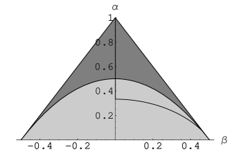
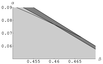
Figure 5: The figure represents the set of bipartite symmetric states which are diagonal on the $J_{z}^{(1)}$ basis. All such states are parametrized by the couple $(\beta,\alpha)$, as given in Eqs. (67) and (68). The light gray region contains separable states. The dark gray region contains the entangled states. The black line is the parametric plot of the double-site reduced output of the $4\to 5$ universal broadcasting, for input Bloch vector length $r$ ranging from 0 to 1. In the magnified window on the right, it is possible to notice that, for nearly pure input, the black line crosses the parabola, namely, the output exhibits bipartite entanglement.

In the phase covariant case it is not possible to carry on the same analysis, since, as we notice in Appendix C, the global output state does not commute with $J_{x}$. However, using the partial traces in Eqs. (104), (105), and (106), it is still possible to evaluate the concurrence numerically.

Figure 6: Entanglement $E$ for the double-site reduced output state, in the cases of universal (l.h.s) and phase covariant (r.h.s) broadcasting from $N=2,4,6,8,10$ to $M=N+1$ copies, as a function of the input Bloch vector length $r$.

In Fig. 6 we report the plots of the entanglement $E$ defined in Ref. wootters as follows

$$E=-\frac{1+\sqrt{1-C^{2}}}{2}\log\frac{1+\sqrt{1-C^{2}}}{2}-\frac{1-\sqrt{1-C^{2}}}{2}\log\frac{1-\sqrt{1-C^{2}}}{2}.$$ (74)

for $N=2,4,6,8,10$ and $M=N+1$ as a function of the input Bloch vector length $r$, both in the universal and phase covariant case. Notice that, contrarily to what happens in the universal case, in the phase covariant case bipartite entanglement vanishes in the limit of pure input states. The absolute value of $C$ goes to zero for increasing number $N$ of input copies.

VI Conclusions and further developments

In this paper we studied symmetric broadcasting maps, where $N$ input qubits initially prepared in the same mixed state are transformed into an output state of $M$ qubits, all described by the same density operator. We considered covariant maps and we investigated in particular the universally covariant case and the phase covariant case. We have shown that for sufficiently mixed initial states and for $N\geqslant 3$ it is also possible to partially purify the single qubit output density operator in the broadcasting operation. Such a new process was named superbroadcasting.

The new superbroadcasting channels open numerous interesting theoretical problems. The first problem is to extend the map to any dimension $d>2$ and to different covariance groups. Indeed, for special cases it is easy to see that increasing the dimensionality and/or reducing the set of states to be broadcast makes superbroadcasting possible with smaller $N$, and even with $N=2$ input states. As a matter of fact, this is the case of universally covariant superbroadcasting from $N=4$ to $M=6$, which can also be regarded as superbroadcasting for $d=4$ for special states of the form $\rho\otimes\rho$, and for the covariance group $\mathbb{SU}(2)\times\mathbb{SU}(2)$. The case of dimension $d=4$ is most interesting, since it can be exploited to improve entanglement for bipartite states of qubits. Also the infinite dimensional case (the so-called “continuous variables”) turns out to be interesting, and easily feasible experimentally cvsb . It should be emphasized that for dimension $d\geq 3$ there are many ways of increasing purity, and certainly the most interesting case is the purification along the mixing direction of a noisy channel (notice that most channels do not correlate, whence the produced state is the tensor product of identical mixed states).

Another major problem is the analysis of the detrimental correlations between two outputs, e. g. to establish whether they are quantum or classical. These correlations are exotic, in the sense that instead of increasing the local mixing as usual, they reduce it. Such mechanism is new, and deserves a more thorough analysis. An interesting issue, for example, is that they cannot be erased leaving the local state unchanged (the de-correlating map—which sends a state to the tensor product of its partial traces—is non linear), and this raises the problem of the optimal de-correlating channel, which optimizes the fidelity between the input and the output local state. Such optimal channel can be derived using the same technique for optimal covariant maps used in the present paper.

Finally, distributing quantum information—and in particular superbroadcasting—raises the new problem of the trade-off between broadcasting and cryptographic security. Indeed, on one side, the presence of many identical uses seems to open more possibilities of eavesdropping, however the detrimental correlations may drastically reduce such possibility, and the opportunity of detecting the eavesdropping on the joint output state may be exploited to increase the security.

Appendix A Decomposition of $\rho^{\otimes N}$

The global density operator $\rho^{\otimes N}$ is clearly invariant under permutations of the $N$ qubits, and, according to the Schur-Weyl duality, it can be represented by the Wedderburn decomposition (10)

$$\rho^{\otimes N}=\bigoplus_{j=j_{0}}^{N/2}\rho_{j}\otimes\openone_{d_{j}},$$ (75)

where $\rho_{j}$ is a state on $\mathscr{H}_{j}$. In order to evaluate $\rho_{j}$ it is sufficient to evaluate the matrix elements $\langle jm|\otimes\langle\alpha|\rho^{\otimes N}|jm^{\prime}\rangle\otimes|\alpha\rangle$, where $|jm\rangle$ are eigenstates of $J_{z}$ in the $j$ representation, and $|\alpha\rangle$ is an arbitrary state in $\mathbb{C}^{d_{j}}$. For the sake of simplicity we can suppose that the state $\rho$ has the Bloch form $\frac{1}{2}(\openone+r\sigma_{z})$. The problem is now to choose $|\alpha\rangle$ in a suitable way. It turns out that a clever choice is given by

$$|jm\rangle\otimes|\alpha\rangle=|jm\rangle_{2j}\otimes|\Psi^{-}\rangle^{\otimes\frac{N-2j}{2}},$$ (76)

where the subscript $2j$ means that $|jm\rangle_{2j}$ is a vector in the symmetric subspace of the first $2j$ qubits, while $|\Psi^{-}\rangle$ is a singlet, supporting an invariant representation on a couple of qubit spaces. Notice that in Eq. (76) the tensor product on the l.h.s. refers to the “abstract” subspace $\mathscr{H}_{j}\otimes\mathbb{C}^{d_{j}}$ in the Wedderburn decomposition, whereas the one on the r.h.s. refers to the decomposition $(\mathbb{C}^{2})^{\otimes 2j}\otimes(\mathbb{C}^{2})^{\otimes(N-2j)}$ grouping separately the first $2j$ qubits and the remaining $N-2j$. Moreover, since the chosen density operator $\rho^{\otimes N}$ commutes with the total $J_{z}$, given by the following expression

$$J_{z}=\bigoplus_{j=j_{0}}^{N/2}J_{z}^{(j)}\otimes\openone_{d_{j}}=\bigoplus_{j=j_{0}}^{N/2}\sum_{m=-j}^{j}m|jm\rangle\langle jm|\otimes\openone_{d_{j}},$$ (77)

then $\rho_{j}$ commutes with $J_{z}^{(j)}$, which implies that $\rho_{j}$ is diagonal on the eigenstates $|jm\rangle$ of $J_{z}^{(j)}$. Therefore we can write

$$(\rho_{j})_{mm}=\;{}_{2j}\langle jm|\rho^{\otimes 2j}|jm\rangle_{2j}\ \left(\langle\Psi^{-}\left|\rho^{\otimes 2}\right|\Psi^{-}\rangle\right)^{\frac{N-2j}{2}}\,.$$ (78)

Since $|jm\rangle_{2j}$ is symmetric, it is a linear combination of factorized vectors with $(j+m)$ qubits in the $|1/2,1/2\rangle$ state and $(j-m)$ in the state $|1/2,-1/2\rangle$. As a consequence we can also write

$$\rho^{\otimes 2j}|jm\rangle_{2j}=r_{+}^{j+m}r_{-}^{j-m}|jm\rangle_{2j}\,,$$ (79)

where $r_{\pm}=\frac{1\pm r}{2}$. By analogous arguments it follows that

$$\rho^{\otimes 2}|\Psi^{-}\rangle=r_{+}r_{-}|\Psi^{-}\rangle\,.$$ (80)

The matrix element $(\rho_{j})_{mm}$ has the following expression

$$(\rho_{j})_{mm}=r_{+}^{j+m}r_{-}^{j-m}(r_{+}r_{-})^{N/2-j}=(r_{+}r_{-})^{N/2}\left(\frac{r_{+}}{r_{-}}\right)^{m},$$ (81)

and the decomposition of $\rho^{\otimes N}$ is finally given by Cirac99

$$\rho^{\otimes N}=(r_{+}r_{-})^{N/2}\bigoplus_{j=j_{0}}^{N/2}\sum_{m=-j}^{j}\left(\frac{r_{+}}{r_{-}}\right)^{m}|jm\rangle\langle jm|\otimes\openone_{d_{j}}\,.$$ (82)

Notice that this expression exhibits a singularity for $r=1$ due to the rearrangement of terms (81). However, a finite limit for $r\to 1$ exists, as it can be seen from the equivalent expression

$$\rho^{\otimes N}=\bigoplus_{j=j_{0}}^{N/2}(r_{+}r_{-})^{N/2-j}\sum_{m=-j}^{j}r_{+}^{j+m}r_{-}^{j-m}|jm\rangle\langle jm|\otimes\openone_{d_{j}}\,,$$ (83)

which exhibits no singularities.

Appendix B Formulae for the scaling factors

In this Appendix we will derive the explicit form of the scaling factor for the universal and phase covariant cases.

B.1 Universal case

In order to calculate $p^{N,M}(r)$ we start rewriting Eq. (40) as

$$\operatorname{Tr}\left[\left(J_{z}^{(j)}\otimes|ln\rangle\langle ln|\right)P^{J}_{j,l}\right]=\operatorname{Tr}\left[|ln\rangle\langle ln|\operatorname{Tr}_{j}\left[\left(J_{z}^{(j)}\otimes\openone_{2l+1}\right)\ P^{J}_{j,l}\right]\right].$$ (84)

Let us define

$$X_{i}^{(l)}\equiv\operatorname{Tr}_{j}\left[\left(J_{i}^{(j)}\otimes\openone_{2l+1}\right)\ P^{J}_{j,l}\right],$$ (85)

where $i=-1,0,1$, and $X_{0}\doteq X_{z}$. Since

$$\left(U_{g}^{(j)}\otimes U^{(l)}_{g}\right)P^{J}_{j,l}\left(U_{g}^{(j)}\otimes U^{(l)}_{g}\right)^{\dagger}=P^{J}_{j,l},$$ (86)

the set $X_{i}^{(l)}$ transforms according to

$$\begin{split}U^{(l)}_{g}X_{i}^{(l)}{U_{g}^{(l)}}^{\dagger}&=\operatorname{Tr}_{j}\left[\left(U_{g}^{(j)}J_{i}^{(j)}{U_{g}^{(j)}}^{\dagger}\otimes\openone_{2l+1}\right)\ P^{J}_{j,l}\right]\\ &=\operatorname{Tr}_{j}\left[\left(\sum_{k=-1}^{1}(U^{(1)}_{g})_{ik}J_{k}^{(j)}\otimes\openone_{2l+1}\right)\ P^{J}_{j,l}\right]\\ &=\sum_{k=-1}^{1}(U^{(1)}_{g})_{ik}X_{k}^{(l)},\\ \end{split}$$ (87)

and we conclude that $\left\{X_{i}^{(l)}\right\}$ is an irreducible tensor set. It can then be proved by the Wigner-Eckart theorem that $X_{i}^{(l)}=\alpha J_{i}^{(l)}$, and in particular $X_{z}^{(l)}=\alpha J_{z}^{(l)}$. From the last relation and from the identity

$$\frac{1}{2}\left(J_{+}^{(l)}J_{-}^{(l)}+J_{-}^{(l)}J_{+}^{(l)}\right)+\left(J_{z}^{(l)}\right)^{2}=\sum_{i=-1}^{1}a_{i}J_{i}^{(l)}J^{(l)}_{-i}=\left(J^{(l)}\right)^{2}\equiv l(l+1)\openone_{2l+1},$$ (88)

where $a_{-1}=a_{1}=1/2$ and $a_{0}=a_{z}=1$, and $J^{(k)}_{0}\doteq J^{(k)}_{z}$, we have

$$\begin{split}\alpha l(l+1)(2l+1)&=\alpha\sum_{i=-1}^{1}a_{i}\operatorname{Tr}\left[J_{i}^{(l)}J_{-i}^{(l)}\right]\\ &=\sum_{i=-1}^{1}a_{i}\operatorname{Tr}\left[\left(J_{i}^{(j)}\otimes J_{-i}^{(l)}\right)P^{J}_{j,l}\right],\end{split}$$ (89)

By using the well known identity

$$\begin{split}\sum_{i=-1}^{1}a_{i}\left(J_{i}^{(j)}\otimes J^{(l)}_{-i}\right)\ P^{J}_{j,l}&=\frac{1}{2}\left({J^{(J)}}^{2}-{J^{(j)}}^{2}\otimes\openone_{2l+1}-\openone_{2j+1}\otimes{J^{(l)}}^{2}\right)P^{J}_{j,l}\\ &=P^{J}_{j,l}\frac{J(J+1)-j(j+1)-l(l+1)}{2}\,,\end{split}$$ (90)

we can write the explicit form of the coefficient $\alpha$

$$\alpha=\frac{2J+1}{2l+1}\frac{J(J+1)-j(j+1)-l(l+1)}{2l(l+1)}\equiv\frac{2J+1}{2l+1}\beta(J,j,l).$$ (91)

By using the above expression we finally have

$$\operatorname{Tr}\left[\left(J_{z}^{(j)}\otimes|ln\rangle\langle ln|\right)\ P^{J}_{j,l}\right]=n\frac{2J+1}{2l+1}\beta(J,j,l).$$ (92)

B.2 Phase covariant case

Substituting the global output state $\Sigma$ given by Eq. (58) into Eq. (25), it is possible to compute the scaling factor $p^{N,M}(r)$ as

$$\begin{split}p^{N,M}(r)\equiv\frac{r^{\prime}}{r}=&\frac{1}{r}\frac{2}{M}(r_{+}r_{-})^{N/2}\sum_{j,l,k}d_{j}d_{l}\sum_{n,n^{\prime}=-l}^{l}r^{j,l}_{n,n^{\prime},k}\left[J_{x}^{(j)}\right]_{n^{\prime}+k,n+k}\times\\ &\sum_{n^{\prime\prime}=-l}^{l}(W_{l})_{n^{\prime},n^{\prime\prime}}\left(\frac{r_{+}}{r_{-}}\right)^{n^{\prime\prime}}(W_{l}^{\dagger})_{n^{\prime\prime},n},\end{split}$$ (93)

where $(W_{k})_{ab}\equiv\langle k,a|k^{x},b\rangle$ are entries of the Wigner rotation matrix in the $k$ representation which rotates the $z$-components to the $x$-components (in the usual notation, the one that is found, for example, in edmonds , such entries are denoted as $d^{(k)}_{ab}\left(\beta\equiv\frac{\pi}{2}\right)$). In Eq. (93) the sum over $n^{\prime\prime}$ gives the $(n,n^{\prime})$-th matrix element of $\exp(J_{x}^{(l)}\log r_{+}/r_{-})$. Therefore we can write

$$\begin{split}p^{N,M}(r)&=\frac{2}{Mr}(r_{+}r_{-})^{N/2}\sum_{j,l,k}d_{j}d_{l}\sum_{n,n^{\prime}=-l}^{l}r^{j,l}_{n,n^{\prime},k}\left[\exp\left(J_{x}^{(l)}\log\frac{1+r}{1-r}\right)\right]_{n^{\prime},n}\left[J_{x}^{(j)}\right]_{n^{\prime}+k,n+k}\\ &=\frac{4}{Mr}(r_{+}r_{-})^{N/2}\sum_{j,l,k}d_{j}d_{l}\sum_{n=-l}^{l}r^{j,l}_{n,n+1,k}\left[\exp\left(J_{x}^{(l)}\log\frac{1+r}{1-r}\right)\right]_{n,n+1}\left[J_{x}^{(j)}\right]_{n+k,n+k+1},\end{split}$$ (94)

where in the last equality we used the fact that $J_{x}^{(j)}=\sum_{m}m|j^{x},m\rangle\langle j^{x},m|$ has non-null matrix elements only on the second-diagonals, and we multiplied the second line by a factor 2 considering in the sum only one of the two second-diagonals. Notice that all matrix elements in the previous equations are calculated with respect to the $z$-oriented basis $|j^{z},m\rangle\equiv|j,m\rangle$ and $|l^{z},n\rangle\equiv|l,n\rangle$.

Appendix C Reduced output states

C.1 Single-site reduced output states

In this appendix we want to calculate the following partial trace

$$\operatorname{Tr}_{M-1}\left[|jm\rangle\langle jm|\otimes\openone_{d_{j}}\right],$$ (95)

where the operator to be partially traced acts on $\mathscr{H}_{j}\otimes\mathbb{C}^{d_{j}}\subset(\mathbb{C}^{2})^{\otimes M}$, and $|jm\rangle$ are eigenstates of $J_{z}^{(j)}$, as usual. In order to do that, we first decompose the vector $|jm\rangle$ into its components onto $\mathscr{H}_{j-1/2}\otimes\mathscr{H}_{1/2}$ using the Clebsch-Gordan coefficients

$$|jm\rangle=\sqrt{\frac{j+m}{2j}}\left|j-\frac{1}{2},m-\frac{1}{2}\right\rangle\otimes\left|\frac{1}{2},\frac{1}{2}\right\rangle+\sqrt{\frac{j-m}{2j}}\left|j-\frac{1}{2},m+\frac{1}{2}\right\rangle\otimes\left|\frac{1}{2},-\frac{1}{2}\right\rangle,$$ (96)

and then trace the operator $|jm\rangle\langle jm|$ over $\mathscr{H}_{j-1/2}$. In this way we get

$$\operatorname{Tr}_{j-1/2}\left[|jm\rangle\langle jm|\right]=\frac{\openone}{2}+\frac{m}{2j}\sigma_{z}.$$ (97)

We now recall a fact related to the already mentioned Schur-Weyl duality, by which multiplicity spaces $\mathbb{C}^{d_{j}}$ in the Wedderburn decomposition (11) support irreducible representations of the permutation group $\{\Pi_{\sigma}^{M}\}$ of $M$ qubits. Hence, for any operator $O$ on $\mathscr{H}_{j}\otimes\mathbb{C}^{d_{j}}$ one has

$$\sum_{\sigma}\Pi_{\sigma}^{M}O\Pi_{\sigma}^{M}=\frac{M!}{d_{j}}\operatorname{Tr}_{\mathbb{C}^{d_{j}}}[O]\otimes\openone_{d_{j}}.$$ (98)

For convenience, let us write

$$|jm\rangle\langle jm|\otimes\openone_{d_{j}}=\frac{d_{j}}{M!}\sum_{\sigma}\Pi_{\sigma}^{M}\left(|jm\rangle\langle jm|\otimes|\Psi^{-}\rangle\langle\Psi^{-}|^{\otimes\frac{M-2j}{2}}\right)\Pi_{\sigma}^{M},$$ (99)

as we already did in Eq. (76). With this choice, we get:

$$\begin{split}\operatorname{Tr}_{M-1}\left[|j,m\rangle\langle j,m|\otimes\openone_{d_{j}}\right]&=\operatorname{Tr}_{M-1}\left[\frac{d_{j}}{M!}\sum_{\sigma}\Pi_{\sigma}^{M}\left(|j,m\rangle\langle j,m|\otimes|\Psi^{-}\rangle\langle\Psi^{-}|^{\otimes\frac{M-2j}{2}}\right)\Pi_{\sigma}^{M}\right]\\ &=\frac{d_{j}}{M!}\left[(M-1)!(M-2j)\frac{\openone}{2}+(M-1)!2j\left(\frac{\openone}{2}+\frac{m}{2j}\sigma_{z}\right)\right]\\ \end{split}$$ (100)

The first term in the sum comes from excluding from trace one of the $(M-2j)$ qubits in singlet state. The second term in the sum comes from excluding from trace one of the $2j$ qubits in $|jm\rangle$ state, and from Eq. (97). Rearranging the above equation, we get the final expression

$$\operatorname{Tr}_{M-1}\left[|j,m\rangle\langle j,m|\otimes\openone_{d_{j}}\right]=d_{j}\left(\frac{\openone}{2}+\frac{m}{M}\sigma_{z}\right).$$ (101)

C.2 Properties of single-site output states

Consider the global output state $\Sigma=\mathcal{B}(\rho^{\otimes N})$. If it commutes with the total angular momentum component along the direction $z$, for example, then it is simple to prove that also $\rho^{\prime}=\operatorname{Tr}_{M-1}[\Sigma]$ commutes with $\sigma_{z}$. In fact, from Eq. (101), it is simple to see that

$$\operatorname{Tr}_{M-1}\left[J_{z}^{(j)}\otimes\openone_{d_{j}}\right]\propto\sigma_{z},$$ (102)

for all $j$, and consequently also $\operatorname{Tr}_{M-1}\left[J_{z}\right]\propto\sigma_{z}$.

In the universal case, the global output $\Sigma$ is diagonal on eigenstates of $J_{z}^{(M/2)}$, hence $\rho^{\prime}=\operatorname{Tr}_{M-1}[\Sigma]$ commutes with $\sigma_{z}$, according to previous arguments. In the phase covariant case, it is more difficult to prove on general grounds that $[\rho^{\prime},\sigma_{x}]=0$, since in the phase covariant case $\left[J_{x},\Sigma\right]\neq 0$. The simplest thing we can do is to compute the partial trace of Eqs. (61) and (62) using again Clebsch-Gordan coefficients (96). First of all let us notice that, tracing over $M-1$ qubits, only the terms with $|n-n^{\prime}|\leq 1$ contribute. Among these, the terms with $n=n^{\prime}$ give one factor proportional to $\openone/2$ and one factor proportional to $\sigma_{z}$, whereas terms with $|n-n^{\prime}|=1$ contribute with factors proportional to $\sigma_{x}$, since the matrix of coefficients $\exp\left(J_{x}^{(l)}\log\frac{1+r}{1-r}\right)$ is symmetric, see Eq. (64). Then, posing $\alpha_{k}=0$ without loss of optimality, $\operatorname{Tr}_{M-1}[\Sigma]$ commutes with $\sigma_{x}$.

C.3 Double-site reduced output states

We will show here how to compute the reduced output state of two copies, which is used in Section V to compute the concurrence between two of the $M$ clones. Clearly it does not matter which two clones we are considering, since the global output state is permutation invariant. Using Clebsch-Gordan coefficients, it is possible to decompose a vector in $\mathscr{H}_{j}$ into its components onto $\mathscr{H}_{j-1}\otimes\mathscr{H}_{1}$

$$\begin{split}|jm\rangle=&\sqrt{\frac{(j+m)(j+m-1)}{2j(2j-1)}}|j-1,m-1\rangle|1,1\rangle+\sqrt{\frac{j^{2}-m^{2}}{j(2j-1)}}|j-1,m\rangle|1,0\rangle+\\ &\sqrt{\frac{(j-m)(j-m-1)}{2j(2j-1)}}|j-1,m+1\rangle|1,-1\rangle,\end{split}$$ (103)

and then to compute the partial trace of $|jm\rangle\langle jm^{\prime}|$ over $\mathscr{H}_{j-1}$. For $j=M/2$ we have

$$\operatorname{Tr}_{M-2}\left[|M/2,m\rangle\langle M/2,m|\right]=\begin{pmatrix}\frac{(M-2m)(M-2m-2)}{4M(M-1)}&0&0\\ 0&\frac{M^{2}-4m^{2}}{2M(M-1)}&0\\ 0&0&\frac{(M+2m)(M+2m-2)}{4M(M-1)}\end{pmatrix},$$ (104)

when $|m-m^{\prime}|=1$

$$\begin{split}\operatorname{Tr}_{M-2}&\left[|M/2,m\rangle\langle M/2,m+1|+\textrm{h.c.}\right]=\\ &\begin{pmatrix}0&\frac{(M-2m-2)\sqrt{(M-2m)(M+2m+2)}}{2\sqrt{2}M(M-1)}&0\\ \frac{(M-2m-2)\sqrt{(M-2m)(M+2m+2)}}{2\sqrt{2}M(M-1)}&0&\frac{(M+2m)\sqrt{(M-2m)(M+2m+2)}}{2\sqrt{2}M(M-1)}\\ 0&\frac{(M+2m)\sqrt{(M-2m)(M+2m+2)}}{2\sqrt{2}M(M-1)}&0\end{pmatrix},\end{split}$$ (105)

and $|m-m^{\prime}|=2$,

$$\begin{split}\operatorname{Tr}_{M-2}&\left[|M/2,m\rangle\langle M/2,m+2|+\textrm{h.c.}\right]=\\ &\begin{pmatrix}0&0&\frac{\sqrt{(M-2m)(M+2m+4)(M+2m+2)(M-2m-2)}}{4M(M-1)}\\ 0&0&0\\ \frac{\sqrt{(M-2m)(M+2m+4)(M+2m+2)(M-2m-2)}}{4M(M-1)}&0&0\end{pmatrix}.\end{split}$$ (106)

For $|m-m^{\prime}|\geq 3$, partial trace over $M-2$ copies gives null contribution.

References

• (1) L. Grover, quant-ph/9704012; J I Cirac, A Ekert, S F Huelga, and C. Macchiavello, Phys. Rev. A 59, 4249 (1999).
• (2) C Crepeau, D Gottesman, and A Smith, in Proceedings of the 34th Annual ACM Symposium on Theory of Computing (New York, ACM Press, 2002).
• (3) S C Benjamin and P M Hayden, Phys. Rev. A 64, 030301 (2001).
• (4) W K Wootters, W H Zurek, Nature 299, 802 (1982).
• (5) D Dieks, Phys. Lett. A, 92, 271 (1982).
• (6) H P Yuen, Phys. Lett. A113 405 (1986).
• (7) In Ref. Wootters82 it was shown that the cloning machine violates the superposition principle, which applies to a minimum total number of three states, and hence does not rule out the possibility of cloning two nonorthogonal states. It is violation of unitarity that makes cloning any two nonorthogonal states impossible, as proved in Ref. Yuen . In reference Dieks82 it was shown that the proposal for superluminal communication does not work, proving the impossibility of cloning in this particular context due to linearity of evolution. According to Ref. peres , previous to Refs. Wootters82 ; Dieks82 the anonymous referee’s report of G. Ghirardi to Ref. herbert contained an argument which was a special case of the no-cloning theorem of Refs. Wootters82 ; Dieks82 . More recently, after several attempts of determining the wave function of a single system appeared in the literature, Ref. darianoyuen showed how it is impossible to determine the wave function from a single copy of the system, and connected such impossibility to the no-cloning theorem.
• (8) G M D’Ariano and H P Yuen, Phys. Rev. Lett. 76 2832 (1996).
• (9) N Herbert, Found. Phys. 12, 1171 (1982).
• (10) A Peres, Fortsch. Phys. 51, 458 (2003).
• (11) H Barnum, C M Caves, C A Fuchs, R Jozsa, and B Schumacher, Phys. Rev. Lett. 76 2818 (1996).
• (12) R Clifton, J Bub, and H Halvorson, Found. of Phys. 33 1561 (2003).
• (13) G M D’Ariano, C Macchiavello, and P Perinotti, Phys. Rev. Lett. 95, 060503 (2005).
• (14) R F Werner, Phys. Rev. A 58, 1827 (1998).
• (15) M. Keyl and R. F. Werner, Ann. H. Poincaré, 2, 1 (2001).
• (16) G M D’Ariano, P Perinotti, and M F Sacchi, quant-ph/0602037; G M D’Ariano, P Perinotti, and M F Sacchi, quant-ph/0601114.
• (17) J I Cirac, A K Ekert, and C Macchiavello, Phys. Rev. Lett. 82, 4344-4347 (1999).
• (18) F Buscemi, G M D’Ariano, C Macchiavello, and P Perinotti, in Proceedings of the 13th Quantum Information Technology Symposium (QIT13) (Sendai, Japan, 2005).
• (19) F Buscemi, G M D’Ariano, and M F Sacchi, Phys. Rev. A 68, 042113 (2003).
• (20) A Jamiołkowski, Rep. Math. Phys. 3, 275 (1972); M-D Choi, Lin. Alg. Appl. 10, 285 (1975).
• (21) W Fulton and J Harris, Representation Theory: a First Course (Springer-Verlag, Berlin, 1991).
• (22) A R Edmonds, Angular Momentum in Quantum Mechanics (Princeton University Press, Princeton, 1960).
• (23) V Bužek, M Hillery, and R F Werner, Phys. Rev. A 60, R2626 (1999).
• (24) G M D’Ariano and C Macchiavello, Phys. Rev. A 67, 042306 (2003).
• (25) F Buscemi, G M D’Ariano, and C Macchiavello, Phys. Rev A 72, 062311 (2005).
• (26) W K Wootters, Phys. Rev. Lett. 80, 2245 (1998).
• (27) D Bruß and C Macchiavello, Found. Phys. 33 (11), 1617 (2003).