Universal measurement of quantum correlations of radiation

Abstract

A measurement technique is proposed which, in principle, allows one to observe the general space-time correlation properties of a quantized radiation field. Our method, called balanced homodyne correlation measurement, unifies the advantages of balanced homodyne detection with those of homodyne correlation measurements.

The pioneering photon correlation experiments performed by Hanbury Brown and Twiss Brown and Twiss (1956) in the 1950th have stimulated a series of investigations of the correlation properties of radiation fields. The quantum field theoretical description of the coherence properties of radiation was introduced by Glauber Glauber (1963a). In this approach the considered correlation functions contain equal powers of negative and positive frequency parts of field operators, which is closely related to the possibilities of observation by photon correlation measurements.

A complete description of the quantum statistical properties of radiation also requires the consideration of more general space-time dependent correlation functions Mandel and Wolf (1965); Klauder and Sudarshan (1968); Peřina (1972); Mandel and Wolf (1995), which are composed of unequal powers of photon annihilation and creation operators. Phase-sensitive correlations of such a type are not directly accessible by photoelectric detection. In principle, they could be observed by transmitting the radiation, prior to the measurement by photodetectors, through an appropriately chosen nonlinear medium Mandel and Wolf (1995). The realization of such measurements is difficult, in particular, when microscopic fields to be measured are too weak for causing the needed nonlinear effects.

Usually phase-sensitive radiation properties are measured by homodyne detection Yuen and Shapiro (1978), where the fields to be measured are superimposed with a coherent reference field, the so-called local oscillator. The methods of balanced homodyne tomography Smithey et al. (1993) and of unbalanced homodyning Wallentowitz and Vogel (1996) allow one to reconstruct the quantum state of an effective single-mode radiation field. The reconstruction of moments has also been considered Richter (1993). More complex methods of multiport homodyning allow one to observe space-time dependent correlations vogel (1995). However, involved reconstruction methods are needed and one obtains only insight in smoothed quantum states, due to noise effects caused by imperfect detection, for details see Welsch et al. (1999) and references therein.

Some special radiation properties composed of unequal orders of annihilation and creation operators can be measured by homodyne correlation techniques Vogel (1991). In this case imperfect detection does not contaminate the detected correlation functions. The method has been further developed for the measurement of arbitrary moments of a single-mode radiation field Shchukin and Vogel (2005a), with the aim to characterize the nonclassical properties of radiation. However, the use of a weak local oscillator makes it difficult to determine moments of high orders.

Why is the accurate determination of space-time dependent correlation functions of radiation fields, including those composed of unequal powers of annihilation and creation operators, of interest? It would lead to new possibilities to study the general (high-order) quantum coherence properties of radiation sources, including the dynamical properties and the spatial irradiation characteristics. New types of time-dependent nonclassical correlation properties could be investigated, which generalize known effects like photon antibunching Kimble et al. (1977). Last but not least, the characterization of entanglement of continuous quantum states can been based on such correlation functions Shchukin and Vogel (2005b). Hence their measurement is of great interest for any kind of application of nonclassical and, in particular, of entangled radiation fields.

In this letter we propose a method for observing the most general normally- and time-ordered correlation functions of radiation fields. It combines advantages of balanced homodyning with those of homodyne correlation measurements in a method to be called balanced homodyne correlation (BHC) measurement. A chosen correlation function is determined by a fixed number of photodetectors, so that imperfect detection does not lead to smoothing effects. Since a strong local oscillator can be used in the BHC method, the signal-to-noise ratio allows to determine high-order correlation functions.

Let us consider the general correlation function $\mathcal{G}^{(n,m)}(x_{1},\ldots,x_{n},y_{1},\ldots,y_{m})$ of an electromagnetic field,

$$\begin{split}\mathcal{G}^{(n,m)}(x_{1},&\ldots,x_{n},y_{1},\ldots,y_{m})=\\ &\left\langle{\rm\raisebox{-2.0pt}{$\>\stackrel{{\scriptstyle\scriptstyle\circ}}{{\scriptstyle\circ}}\>$}}\prod^{n}_{k=1}\hat{\mathcal{E}}^{(-)}(x_{k})\prod^{m}_{l=1}\hat{\mathcal{E}}^{(+)}(y_{l}){\rm\raisebox{-2.0pt}{$\>\stackrel{{\scriptstyle\scriptstyle\circ}}{{\scriptstyle\circ}}\>$}}\right\rangle,\end{split}$$ (1)

where $x_{k}=(\mathbf{r}_{k},t_{k})$, $y_{l}=(\mathbf{s}_{l},\tau_{l})$ refer to both space and time points. The operator $\hat{\mathcal{E}}^{(-)}$ ($\hat{\mathcal{E}}^{(+)}$) denotes the negative (positive) frequency part of the electric field operator containing the photon creation (annihilation) operators. The notation $\>\stackrel{{\scriptstyle\scriptstyle\circ}}{{\scriptstyle\circ}}\>$$\>\stackrel{{\scriptstyle\scriptstyle\circ}}{{\scriptstyle\circ}}\>$, as used in Vogel et al. (2001), means that field operators are to be written in normal order ($\hat{\mathcal{E}}^{(-)}$ to the left of $\hat{\mathcal{E}}^{(+)}$), and time order (time arguments increasing to the right in products of $\hat{\mathcal{E}}^{(-)}$ and to the left in products of $\hat{\mathcal{E}}^{(+)}$). For simplicity we restrict ourselves to the case of one polarization, the extension to different polarizations is straightforward.

Let us start with the simplest case of one and the same space-time point in all the field operators in the expression (1): $x_{1}=\ldots=x_{n}=y_{1}=\ldots=y_{m}=(\mathbf{r},t)$. In such a case the correlation function (1) reads as

$$\mathcal{G}^{(n,m)}(\mathbf{r},t)=\left\langle\hat{\mathcal{E}}^{(-)}(\mathbf{r},t)^{n}\hat{\mathcal{E}}^{(+)}(\mathbf{r},t)^{m}\right\rangle.$$ (2)

Here the field operators are already normally ordered and time-ordering becomes meaningless. The correlation function (2) can be measured with the device shown in Fig. 1. This device is parameterized by an integer, the number of levels or depth of the device. The measurement device ($\mathrm{MD}$) of the depth $d$ we denote by $\mathrm{MD}_{d}$. It has $2^{d}$ photodetectors and can be composed recursively of two devices $\mathrm{MD}^{\prime}_{d-1}$ and $\mathrm{MD}^{\prime\prime}_{d-1}$ of lower depth $d-1$, cf. Fig. 2. The elementary building block of our setup is the lowest order device $\mathrm{MD}_{1}$. Roughly speaking, $\mathrm{MD}_{d}$ can be constructed by replacing both photodetectors of $\mathrm{MD}_{1}$ by $\mathrm{MD}_{d-1}$. All the beamsplitters of the device $\mathrm{MD}_{d}$ are assumed to be symmetric $50$%-$50$% and all the photodetectors to have the same quantum efficiency $\eta$. This can be realized by balancing them with polarizers.

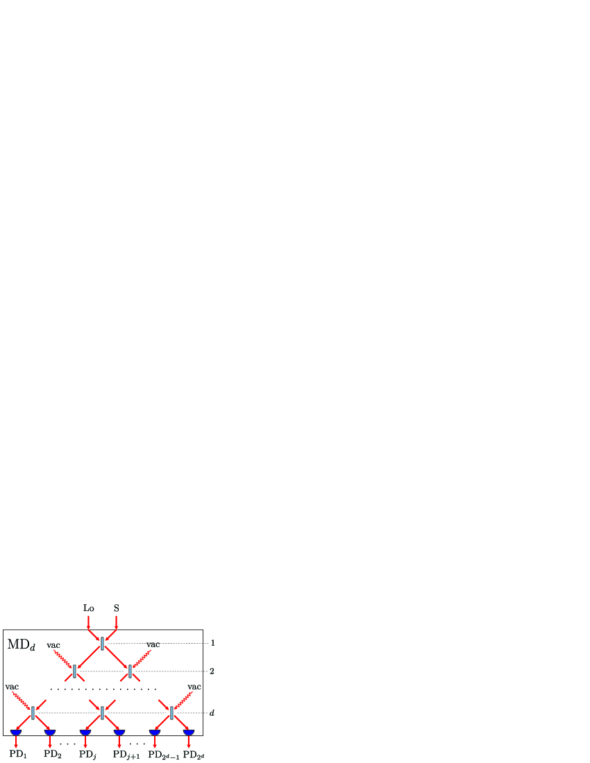
Figure 1: Basic measurement device $\mathrm{MD}_{d}$.

In the BHC approach the device $\mathrm{MD}_{d}$ allows us to measure the correlations (2) with $n+m\leqslant 2^{d-1}$, so that the minimal depth $d$ necessary to measure the moments (2) with given $n$ and $m$ is $d=\lceil\log_{2}(n+m)\rceil+1$ ($\lceil x\rceil$ is the smallest integer number greater or equal to $x$). We assume the local oscillator to be in a coherent state

$$\Bigl{\langle}\hat{\mathcal{E}}^{(-)}_{\mathrm{LO}}\ldots\Bigr{\rangle}=Ee^{-i(\omega t+\varphi_{\mathrm{LO}})},\quad\Bigl{\langle}\ldots\hat{\mathcal{E}}^{(+)}_{\mathrm{LO}}\Bigr{\rangle}=Ee^{i(\omega t+\varphi_{\mathrm{LO}})}.$$ (3)

One can easily see that the field operators $\hat{\mathcal{E}}^{(\pm)\prime}_{j}$ ($\hat{\mathcal{E}}^{(\pm)\prime\prime}_{j}$) detected by $j$-th photodetector $\mathrm{PD}^{\prime}_{j}$ ($\mathrm{PD}^{\prime\prime}_{j}$) of the left subdevice $\mathrm{MD}^{\prime}_{d-1}$ (right subdevice $\mathrm{MD}^{\prime\prime}_{d-1}$) are proportional to the operators $\hat{\mathcal{E}}^{(\pm)}_{+}$ ($\hat{\mathcal{E}}^{(\pm)}_{-}$):

$$\hat{\mathcal{E}}^{(\pm)\prime}_{j}=\frac{e^{\pm i\Phi_{j}}}{\sqrt{2^{d-1}}}\hat{\mathcal{E}}^{(\pm)}_{+}+\mathrm{vac},\quad\hat{\mathcal{E}}^{(\pm)\prime\prime}_{j}=\frac{e^{\pm i\Phi_{j}}}{\sqrt{2^{d-1}}}\hat{\mathcal{E}}^{(\pm)}_{-}+\mathrm{vac},$$ (4)

$j=1,\ldots,2^{d-1}$, the phase $\Phi_{j}$ depends on the path of the signal to the $j$-th photodetector. The operators $\hat{\mathcal{E}}^{(+)}_{\pm}$ read as

$$\hat{\mathcal{E}}^{(+)}_{\pm}=\frac{e^{i\Phi_{\pm}}}{\sqrt{2}}\Bigl{(}\hat{\mathcal{E}}^{(+)}(\mathbf{r},t)\pm i\hat{\mathcal{E}}^{(+)}_{\mathrm{LO}}\Bigr{)},$$ (5)

with $\Phi_{+}-\Phi_{-}=\pi/2$. The symbol $\mathrm{vac}$ in (4) means vacuum terms which play no role in the considered homodyne correlation measurements.

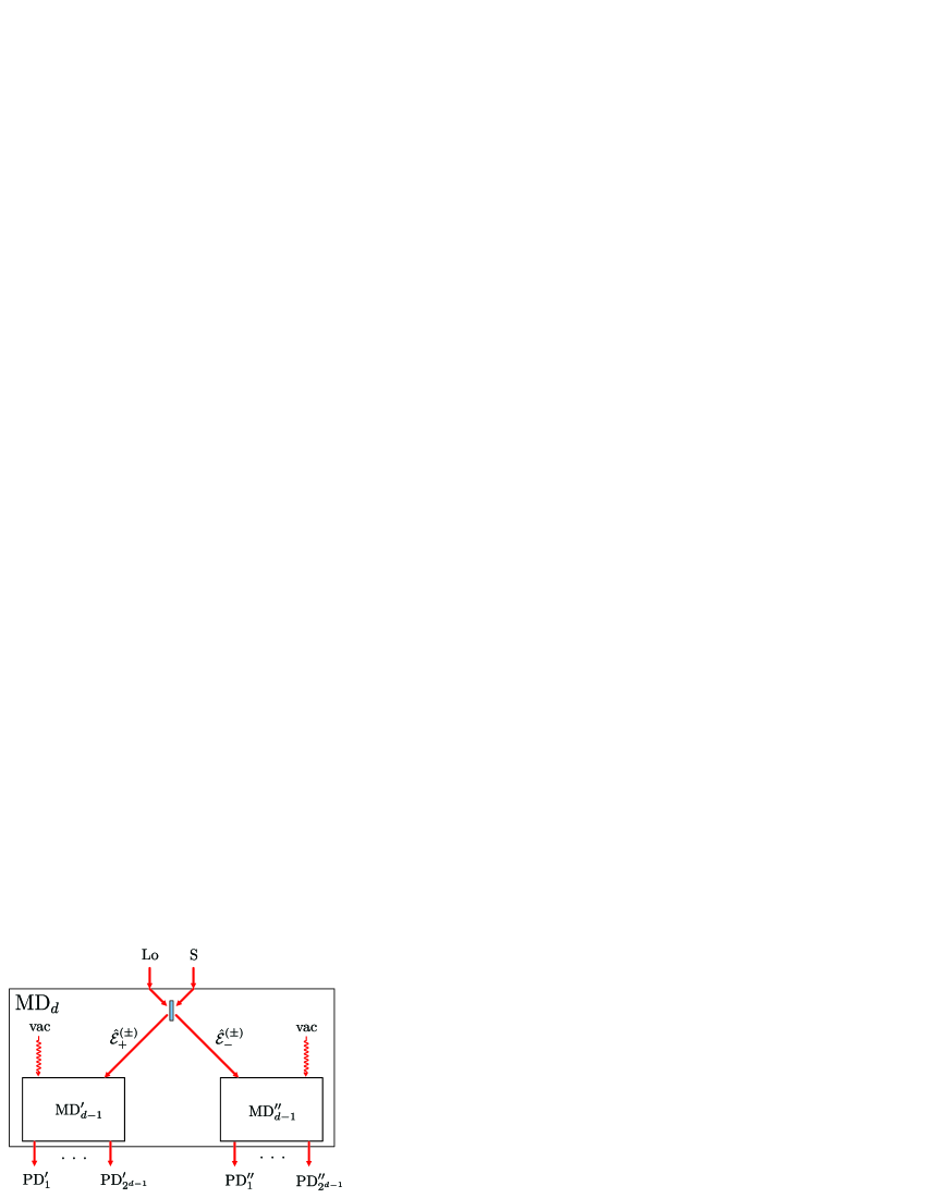
Figure 2: The recursive structure of $\mathrm{MD}_{d}$.

Let us denote by $\Gamma_{j_{1},\ldots,j_{k}}$ the normally-ordered (symbolized by $::$) correlation function of the photodetectors $\mathrm{PD}_{j_{1}},\ldots,\mathrm{PD}_{j_{k}}$,

$$\Gamma_{j_{1},\ldots,j_{k}}=\Bigl{\langle}:\hat{\mathcal{E}}^{(-)}_{j_{1}}\hat{\mathcal{E}}^{(+)}_{j_{1}}\ldots\hat{\mathcal{E}}^{(-)}_{j_{k}}\hat{\mathcal{E}}^{(+)}_{j_{k}}:\Bigr{\rangle},$$ (6)

For any $k=1,\ldots,2^{d-1}$ and for any $l$, $0\leqslant l\leqslant k$, let us select $l$ photodetectors from $\mathrm{MD}^{\prime}_{d-1}$ and $k-l$ from $\mathrm{MD}^{\prime\prime}_{d-1}$ (cf. Fig. 2) and measure their correlation function. Due to the relations (4) such a correlation function depends only on the numbers $k$ and $l$ but not on the individual photodetectors chosen. We denote it by $\Gamma^{(k)}_{l}$, using Eq. (4) it reads as

$$\Gamma^{(k)}_{l}=2^{-k(d-1)}\Bigl{\langle}:\hat{\mathcal{N}}^{l}_{+}\hat{\mathcal{N}}^{k-l}_{-}:\Bigr{\rangle}.$$ (7)

The operators $\hat{\mathcal{N}}_{+}$ and $\hat{\mathcal{N}}_{-}$ are defined analogously to the photon number operator of a single-mode field,

$$\hat{\mathcal{N}}_{\pm}=\hat{\mathcal{E}}^{(-)}_{\pm}\hat{\mathcal{E}}^{(+)}_{\pm}=\frac{1}{2}\Bigl{(}\hat{\mathcal{E}}^{(-)}\hat{\mathcal{E}}^{(+)}\pm E\hat{\mathcal{X}}_{\varphi}+E^{2}\Bigr{)},$$ (8)

and $\hat{\mathcal{X}}_{\varphi}$ corresponds to the quadrature operator,

$$\hat{\mathcal{X}}_{\varphi}=\hat{\tilde{\mathcal{E}}}^{(+)}e^{-i\varphi}+\hat{\tilde{\mathcal{E}}}^{(-)}e^{i\varphi},$$ (9)

with $\hat{\tilde{\mathcal{E}}}^{(\pm)}=\hat{\mathcal{E}}^{(\pm)}e^{\pm i\omega t}$ being slowly varying fields and $\varphi=\varphi_{\mathrm{LO}}+\pi/2$.

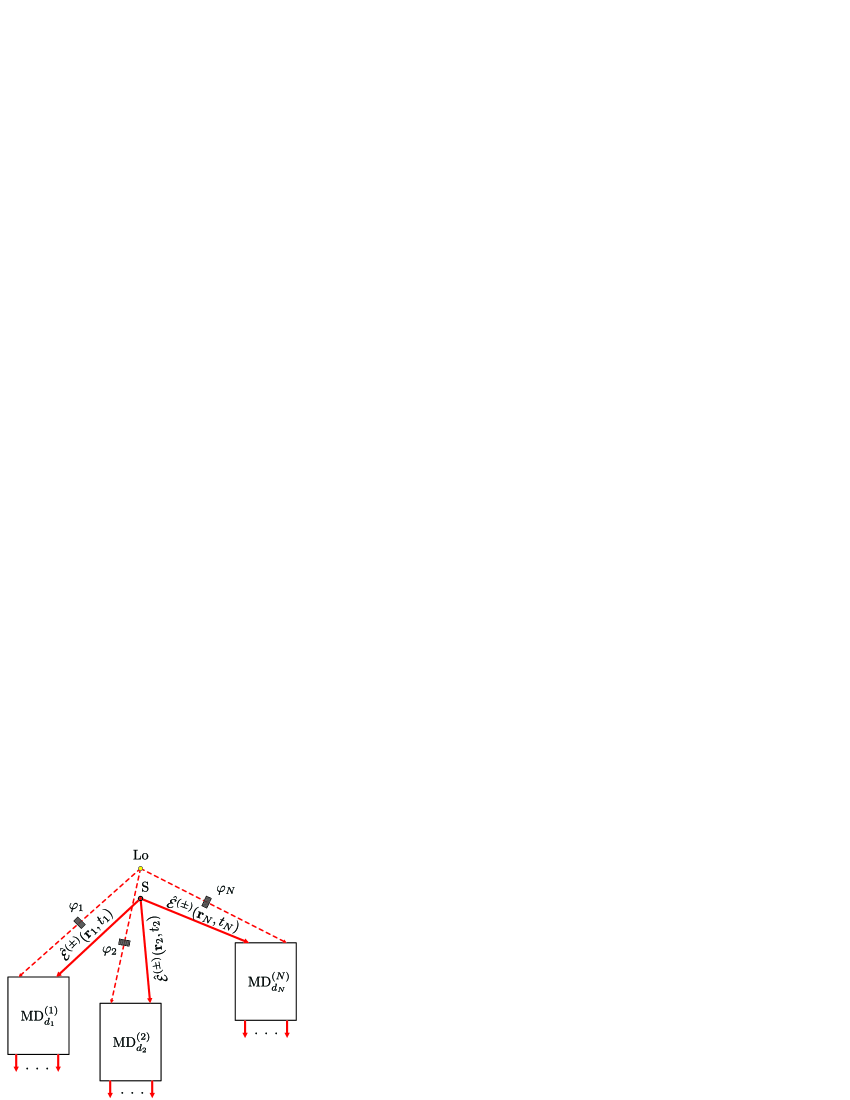
Figure 3: Measurement scheme for space-time correlations.

Let us chose one correlation function $\Gamma^{(k)}_{l}$ for each $l=0,1,\ldots,k$ and combine them as

$$F^{(k)}=\sum^{k}_{l=0}(-1)^{k-l}\binom{k}{l}\Gamma^{(k)}_{l}.$$ (10)

It is important to note that all the terms in this sum are proportional to $k$-th power of the quantum efficiency of the photodetectors. Using the binomial formula we obtain

$$F^{(k)}(\varphi)=2^{-kd}\Bigl{\langle}:(\hat{\mathcal{N}}_{+}-\hat{\mathcal{N}}_{-})^{k}:\Bigr{\rangle}=2^{-kd}E^{k}\Bigl{\langle}:\hat{\mathcal{X}}^{k}_{\varphi}:\Bigr{\rangle},$$ (11)

which represents the set of BHC data to be analyzed. The dependence of the quantity $F^{(k)}$ on the phase $\varphi$ is given explicitly: $F^{(k)}=F^{(k)}(\varphi)$. According the definition of the operator $\hat{\mathcal{X}}_{\varphi}$, the normally ordered power $:\hat{\mathcal{X}}^{k}_{\varphi}:$ can be expanded as

$$\langle:\hat{\mathcal{X}}^{k}_{\varphi}:\rangle=\sum^{k}_{l=0}\binom{k}{l}\Bigl{\langle}\hat{\tilde{\mathcal{E}}}^{(-)l}\hat{\tilde{\mathcal{E}}}^{(+)k-l}\Bigr{\rangle}e^{-i(k-2l)\varphi}.$$ (12)

Hence, the moments $\Bigl{\langle}\hat{\tilde{\mathcal{E}}}^{(-)n}\hat{\tilde{\mathcal{E}}}^{(+)m}\Bigr{\rangle}$ can be obtained directly by Fourier transforming the BHC data:

$$\Bigl{\langle}\hat{\tilde{\mathcal{E}}}^{(-)n}\hat{\tilde{\mathcal{E}}}^{(+)m}\Bigr{\rangle}\sim\int^{2\pi}_{0}F^{(n+m)}(\varphi)e^{-i(n-m)\varphi}\,d\varphi.$$ (13)

The moments of the original field are given by

$$\Bigl{\langle}\hat{\mathcal{E}}^{(-)n}\hat{\mathcal{E}}^{(+)m}\Bigr{\rangle}=\Bigl{\langle}\hat{\tilde{\mathcal{E}}}^{(-)n}\hat{\tilde{\mathcal{E}}}^{(+)m}\Bigr{\rangle}e^{i(n-m)\omega t}.$$ (14)

Once we know how to measure the moments (2) in a single space-time point, the method can be extended to the general space-time correlations (1). All field operators in the same space-time points can be grouped together and after a proper permutation any correlation function (1) can be represented in the form

$$\mathcal{G}=\left\langle{\rm\raisebox{-2.0pt}{$\>\stackrel{{\scriptstyle\scriptstyle\circ}}{{\scriptstyle\circ}}\>$}}\prod^{N}_{i=1}\hat{\mathcal{E}}^{(-)n_{i}}(\mathbf{r}_{i},t_{i})\hat{\mathcal{E}}^{(+)m_{i}}(\mathbf{r}_{i},t_{i}){\rm\raisebox{-2.0pt}{$\>\stackrel{{\scriptstyle\scriptstyle\circ}}{{\scriptstyle\circ}}\>$}}\right\rangle,$$ (15)

where some of the $n_{i}$ or $m_{i}$ can be zero. For example, the correlation function

$$\mathcal{G}^{(1,2)}(x,y,y)=\langle{\rm\raisebox{-2.0pt}{$\>\stackrel{{\scriptstyle\scriptstyle\circ}}{{\scriptstyle\circ}}\>$}}\hat{\mathcal{E}}^{(-)}(x)\hat{\mathcal{E}}^{(+)2}(y){\rm\raisebox{-2.0pt}{$\>\stackrel{{\scriptstyle\scriptstyle\circ}}{{\scriptstyle\circ}}\>$}}\rangle$$ (16)

can be written in the form (15) as

$$\mathcal{G}^{(1,2)}(x,y,y)=\langle{\rm\raisebox{-2.0pt}{$\>\stackrel{{\scriptstyle\scriptstyle\circ}}{{\scriptstyle\circ}}\>$}}\hat{\mathcal{E}}^{(-)1}(x)\hat{\mathcal{E}}^{(+)0}(x)\hat{\mathcal{E}}^{(-)0}(y)\hat{\mathcal{E}}^{(+)2}(y){\rm\raisebox{-2.0pt}{$\>\stackrel{{\scriptstyle\scriptstyle\circ}}{{\scriptstyle\circ}}\>$}}\rangle.$$ (17)

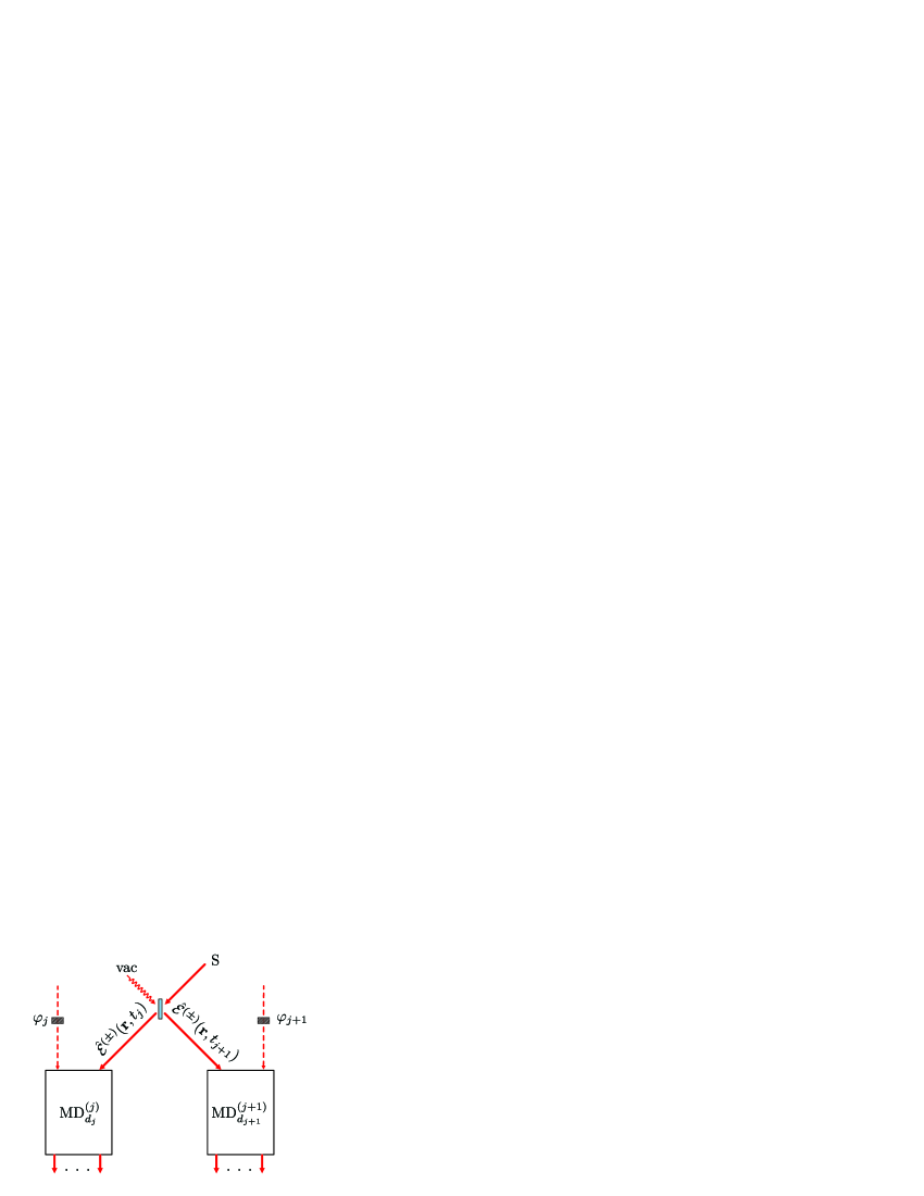
Figure 4: Measurement scheme for time-dependent correlations at equal space points, $\mathbf{r}_{j}=\mathbf{r}_{j+1}=\mathbf{r}$.

Figure 3 illustrates the scheme for measuring the general correlation function (15). The phases $\varphi_{1},\ldots,\varphi_{N}$ of the local oscillator in each channel can be controlled independently by the corresponding phase shifters. For $\mathbf{r}_{j}=\mathbf{r}_{j+1}=\mathbf{r}$ and $t_{j}\not=t_{j+1}$ we split the channel corresponding to the space point $\mathbf{r}$ into two parts as shown in Fig. 4. If more than two space points coincide, we split the signal in the corresponding channel by using the same tree-like combination of beam splitters and photodetectors as in $\mathrm{MD}_{d}$ for a proper $d$, see Fig. 1.

Measuring correlations of photodetectors of all the devices $\mathrm{MD}^{(i)}_{d_{i}}$, one can extract the functions (15) with $n_{i}+m_{i}\leqslant 2^{d_{i}-1}$, $i=1,\ldots,N$. Let us select $k_{i}$ photodetectors from the $i$-th device $\mathrm{MD}^{(i)}_{d_{i}}$ for $i=1,\ldots,N$ and measure the correlation function of all the $K=k_{1}+\ldots+k_{N}$ photodetectors chosen. One can easily see that such a correlation function $\Gamma=\Gamma^{(k_{1}\ldots k_{N})}_{l_{1}\ldots l_{N}}$ has the form

$$\Gamma^{(k_{1}\ldots k_{N})}_{l_{1}\ldots l_{N}}=2^{-P}\left\langle{\rm\raisebox{-2.0pt}{$\>\stackrel{{\scriptstyle\scriptstyle\circ}}{{\scriptstyle\circ}}\>$}}\prod^{N}_{i=1}\hat{\mathcal{N}}^{(i)l_{i}}_{+}(\mathbf{r}_{i},t_{i})\hat{\mathcal{N}}^{(i)k_{i}-l_{i}}_{-}(\mathbf{r}_{i},t_{i}){\rm\raisebox{-2.0pt}{$\>\stackrel{{\scriptstyle\scriptstyle\circ}}{{\scriptstyle\circ}}\>$}}\right\rangle,$$ (18)

where $P=\sum_{i}k_{i}d_{i}$ and $l_{i}$ is the number of those photodetectors of $\mathrm{MD}^{(i)}_{d_{i}}$ that belong to the left subdevice $\mathrm{MD}^{(i)\prime}_{d_{i}-1}$. Generalizing the single-mode approach, one can compose the recorded data in the form

$$F^{(k_{1}\ldots k_{N})}=\sum^{k_{1},\ldots,k_{N}}_{l_{1},\ldots,l_{N}=0}(-1)^{K-L}\binom{k_{1}}{l_{1}}\ldots\binom{k_{N}}{l_{N}}\Gamma^{(k_{1}\ldots k_{N})}_{l_{1}\ldots l_{N}},$$ (19)

where $L=l_{1}+\ldots+l_{N}$, which is equal to

$$\begin{split}F^{(k_{1}\ldots k_{N})}&=2^{-P}\left\langle{\rm\raisebox{-2.0pt}{$\>\stackrel{{\scriptstyle\scriptstyle\circ}}{{\scriptstyle\circ}}\>$}}\prod^{N}_{i=1}(\hat{\mathcal{N}}^{(i)}_{+}(\mathbf{r}_{i},t_{i})-\hat{\mathcal{N}}^{(i)}_{-}(\mathbf{r}_{i},t_{i}))^{k_{i}}{\rm\raisebox{-2.0pt}{$\>\stackrel{{\scriptstyle\scriptstyle\circ}}{{\scriptstyle\circ}}\>$}}\right\rangle\\ &=2^{-P}E^{K}\langle{\rm\raisebox{-2.0pt}{$\>\stackrel{{\scriptstyle\scriptstyle\circ}}{{\scriptstyle\circ}}\>$}}\hat{\mathcal{X}}^{k_{1}}_{\varphi_{1}}(\mathbf{r}_{1},t_{1})\ldots\hat{\mathcal{X}}^{k_{N}}_{\varphi_{N}}(\mathbf{r}_{N},t_{N}){\rm\raisebox{-2.0pt}{$\>\stackrel{{\scriptstyle\scriptstyle\circ}}{{\scriptstyle\circ}}\>$}}\rangle.\end{split}$$ (20)

Using multidimensional Fourier transform one can extract from the function $F^{(k_{1}\ldots k_{N})}=F^{(k_{1}\ldots k_{N})}(\varphi_{1},\ldots,\varphi_{N})$ the correlations (15) or, equivalently, the original form (1) of the space-time dependent field correlation function.

Let us define the characteristic function $C[\mathbf{u}]$ via

$$C[\mathbf{u}]=\left\langle{\rm\raisebox{-2.0pt}{$\>\stackrel{{\scriptstyle\scriptstyle\circ}}{{\scriptstyle\circ}}\>$}}\exp\left(\sum^{N}_{i=1}(u_{i}\hat{\mathcal{E}}^{(-)}(x_{i})-u^{*}_{i}\hat{\mathcal{E}}^{(+)}(x_{i}))\right){\rm\raisebox{-2.0pt}{$\>\stackrel{{\scriptstyle\scriptstyle\circ}}{{\scriptstyle\circ}}\>$}}\right\rangle,$$ (21)

where $\mathbf{u}=(u_{1},\ldots,u_{N})$. The moments (2) are readily derived by

$$\left.\frac{\partial^{n+m}C[\mathbf{u}]}{\partial^{n}u_{i}\partial^{m}u^{*}_{i}}\right|_{\mathbf{u}=0}=\langle{\rm\raisebox{-2.0pt}{$\>\stackrel{{\scriptstyle\scriptstyle\circ}}{{\scriptstyle\circ}}\>$}}\hat{\mathcal{E}}^{(-)n}(x_{i})\hat{\mathcal{E}}^{(+)m}(x_{i}){\rm\raisebox{-2.0pt}{$\>\stackrel{{\scriptstyle\scriptstyle\circ}}{{\scriptstyle\circ}}\>$}}\rangle.$$ (22)

The general correlation functions (15) are given by the general partial derivatives of $C[\mathbf{u}]$ with respect to all the variables. Expanding the characteristic function as

$$C[\mathbf{u}]=\sum^{+\infty}_{n_{i},m_{i}=0}\frac{\langle{\rm\raisebox{-2.0pt}{$\>\stackrel{{\scriptstyle\scriptstyle\circ}}{{\scriptstyle\circ}}\>$}}\prod^{N}_{i=1}\hat{\mathcal{E}}^{(-)n_{i}}(x_{i})\hat{\mathcal{E}}^{(+)m_{i}}(x_{i}){\rm\raisebox{-2.0pt}{$\>\stackrel{{\scriptstyle\scriptstyle\circ}}{{\scriptstyle\circ}}\>$}}\rangle}{\prod^{N}_{i=1}n_{i}!\,m_{i}!},$$ (23)

it is seen that, in principle, the correlation functions (15) completely describe the quantum statistical properties of the radiation field in the chosen space-time points.

Finally, we note that our approach works only for quasimonochromatic fields that are completely recorded by the detectors. More generally, broadband fields could be studied by including spectral correlation measurements as was done for light pulses Beck et al. (2001). This experiment also shows the feasibility of multichannel measurements as needed for our method.

In conclusion, we have proposed a method for measuring general space-time dependent correlation functions of quantized radiation fields. Homodyne correlation measurements are performed and the data are combined and analyzed in a balanced form. The detected correlation functions are insensitive to imperfect detection. By using a strong local oscillator, even higher-order correlations can be determined. This opens new perspectives for the study of nonclassical correlations and, in particular, of entanglement of complex radiation fields.

The authors acknowledge support by the Deutsche Forschungsgemeinschaft through SFB 652 and GK 567.

References

• Brown and Twiss (1956) R. H. Brown and R. Q. Twiss, Nature 177, 27 (1956); Proc. Roy. Soc. (London) A242, 300 (1957); ibid. A243, 291 (1958).
• Glauber (1963a) R. J. Glauber, Phys. Rev. 130, 2529 (1963a); ibid. 131, 2766 (1963b).
• Mandel and Wolf (1965) L. Mandel and E. Wolf, Rev. Mod. Phys. 37, 231 (1965).
• Klauder and Sudarshan (1968) J. R. Klauder and E. C. G. Sudarshan, Fundamentals of Quantum Optics (W. A. Benjamin, New York, 1968).
• Peřina (1972) J. P. Peřina, Coherence of light (Van Nostrand Reinhold, London, 1972).
• Mandel and Wolf (1995) L. Mandel and E. Wolf, Optical Coherence and Quantum Optics (Cambridge, 1995).
• Yuen and Shapiro (1978) H. P. Yuen and J. H. Shapiro, IEEE Trans. Inf. Theory 24, 657 (1978); J. H. Shapiro, H. P. Yuen, and A. Mata, IEEE Trans. Inf. Theory 25, 179 (1979).
• Smithey et al. (1993) D. T. Smithey, M. Beck, M. G. Raymer, and A. Faridani, Phys. Rev. Lett. 70, 1244 (1993); A. I. Lvovsky, H. Hansen, T. Aichele, O. Benson, J. Mlynek, and S. Schiller, Phys. Rev. Lett. 87, 050402 (2001); A. Zavatta, S. Viciani, and M. Bellini, Science 306, 660 (2004);
• Wallentowitz and Vogel (1996) S. Wallentowitz and W. Vogel, Phys. Rev. A 53, 4528 (1996a); K. Banaszek and K. Wódkiewicz, Phys. Rev. Lett. 76, 4344 (1996a).
• Richter (1993) Th. Richter, Phys. Rev. A 53, 1197 (1996).
• vogel (1995) H. Kühn, D.-G. Welsch, and W. Vogel, Phys. Rev. A 51, 4240 (1995); T. Opatrný, D.-G. Welsch, and W. Vogel, Phys. Rev. A 55, 1416 (1997); D. F. McAlister, and M. G. Raymer, J. Mod. Opt. 44, 2359 (1997); Th. Richter, J. Mod. Opt. 44, 2385 (1997);
• Welsch et al. (1999) D.-G. Welsch, W. Vogel, and T. Opatrný, in Progress in Optics, edited by E. Wolf (Elsevier, Amsterdam, 1999), vol. XXXIX, p. 63.
• Vogel (1991) W. Vogel, Phys. Rev. Lett. 67, 2450 (1991); Phys. Rev. A 51, 4160 (1995); H. J. Carmichael, H. M. Castro-Beltran, G. T. Foster, and L. A. Orozco, Phys. Rev. Lett. 85, 1855 (2000).
• Shchukin and Vogel (2005a) E. V. Shchukin and W. Vogel, Phys. Rev. A 72, 043808 (2005a).
• Kimble et al. (1977) H. J. Kimble, M. Dagenais, and L. Mandel, Phys. Rev. Lett. 39, 691 (1977).
• Shchukin and Vogel (2005b) E. Shchukin and W. Vogel, Phys. Rev. Lett. 95, 230502 (2005b).
• Vogel et al. (2001) W. Vogel and D.-G. Welsch, Quantum Optics (Wiley-VCH, 2006), 3rd ed.
• Beck et al. (2001) M. Beck, C. Dorrer, and I. A. Walmsley, Phys. Rev. Lett. 87, 253601 (2001).